Consent Manager Tag v2.0 (for TCF 2.0) -->
Farnell PDF

 ADC-System on the ADMCF32X Application Note (ANF32X ... - Analog Devices
ADC-System on the ADMCF32X Application Note (ANF32X ... - Analog Devices
- Revenir à l'accueil


")

Farnell Element 14 :


See the trailer for the next exciting episode of The Ben Heck show. Check back on Friday to be among the first to see the exclusive full show on element…

Connect your Raspberry Pi to a breadboard, download some code and create a push-button audio play project.


Puce électronique / Microchip :


Sans fil - Wireless :


Texas instrument :


Ordinateurs :


Logiciels :


Tutoriels :


Autres documentations :
![[TXT]](http://www.audentia-gestion.fr/icons/text.gif)
Farnell-NA555-NE555-..> 08-Sep-2014 07:33 1.5M
Farnell-AD9834-Rev-D..> 08-Sep-2014 07:32 1.2M
Farnell-MSP430F15x-M..> 08-Sep-2014 07:32 1.3M
Farnell-AD736-Rev-I-..> 08-Sep-2014 07:31 1.3M
Farnell-AD8307-Data-..> 08-Sep-2014 07:30 1.3M
Farnell-Single-Chip-..> 08-Sep-2014 07:30 1.5M
Farnell-Quadruple-2-..> 08-Sep-2014 07:29 1.5M
Farnell-ADE7758-Rev-..> 08-Sep-2014 07:28 1.7M
Farnell-MAX3221-Rev-..> 08-Sep-2014 07:28 1.8M
Farnell-USB-to-Seria..> 08-Sep-2014 07:27 2.0M
Farnell-AD8313-Analo..> 08-Sep-2014 07:26 2.0M
Farnell-SN54HC164-SN..> 08-Sep-2014 07:25 2.0M
Farnell-AD8310-Analo..> 08-Sep-2014 07:24 2.1M
Farnell-AD8361-Rev-D..> 08-Sep-2014 07:23 2.1M
Farnell-2N3906-Fairc..> 08-Sep-2014 07:22 2.1M
Farnell-AD584-Rev-C-..> 08-Sep-2014 07:20 2.2M
Farnell-ADE7753-Rev-..> 08-Sep-2014 07:20 2.3M
Farnell-TLV320AIC23B..> 08-Sep-2014 07:18 2.4M
Farnell-AD586BRZ-Ana..> 08-Sep-2014 07:17 1.6M
Farnell-STM32F405xxS..> 27-Aug-2014 18:27 1.8M
Farnell-MSP430-Hardw..> 29-Jul-2014 10:36 1.1M
Farnell-LM324-Texas-..> 29-Jul-2014 10:32 1.5M
Farnell-LM386-Low-Vo..> 29-Jul-2014 10:32 1.5M
Farnell-NE5532-Texas..> 29-Jul-2014 10:32 1.5M
Farnell-Hex-Inverter..> 29-Jul-2014 10:31 875K
Farnell-AT90USBKey-H..> 29-Jul-2014 10:31 902K
Farnell-AT89C5131-Ha..> 29-Jul-2014 10:31 1.2M
Farnell-MSP-EXP430F5..> 29-Jul-2014 10:31 1.2M
Farnell-Explorer-16-..> 29-Jul-2014 10:31 1.3M
Farnell-TMP006EVM-Us..> 29-Jul-2014 10:30 1.3M
Farnell-Gertboard-Us..> 29-Jul-2014 10:30 1.4M
Farnell-LMP91051-Use..> 29-Jul-2014 10:30 1.4M
Farnell-Thermometre-..> 29-Jul-2014 10:30 1.4M
Farnell-user-manuel-..> 29-Jul-2014 10:29 1.5M
Farnell-fx-3650P-fx-..> 29-Jul-2014 10:29 1.5M
Farnell-2-GBPS-Diffe..> 28-Jul-2014 17:42 2.7M
Farnell-LMT88-2.4V-1..> 28-Jul-2014 17:42 2.8M
Farnell-Octal-Genera..> 28-Jul-2014 17:42 2.8M
Farnell-Dual-MOSFET-..> 28-Jul-2014 17:41 2.8M
Farnell-TLV320AIC325..> 28-Jul-2014 17:41 2.9M
Farnell-SN54LV4053A-..> 28-Jul-2014 17:20 5.9M
Farnell-TAS1020B-USB..> 28-Jul-2014 17:19 6.2M
Farnell-TPS40060-Wid..> 28-Jul-2014 17:19 6.3M
Farnell-TL082-Wide-B..> 28-Jul-2014 17:16 6.3M
Farnell-RF-short-tra..> 28-Jul-2014 17:16 6.3M
Farnell-maxim-integr..> 28-Jul-2014 17:14 6.4M
Farnell-TSV6390-TSV6..> 28-Jul-2014 17:14 6.4M
Farnell-Fast-Charge-..> 28-Jul-2014 17:12 6.4M
Farnell-NVE-datashee..> 28-Jul-2014 17:12 6.5M
Farnell-Excalibur-Hi..> 28-Jul-2014 17:10 2.4M
Farnell-Excalibur-Hi..> 28-Jul-2014 17:10 2.4M
Farnell-REF102-10V-P..> 28-Jul-2014 17:09 2.4M
Farnell-TMS320F28055..> 28-Jul-2014 17:09 2.7M
Farnell-MULTICOMP-Ra..> 22-Jul-2014 12:35 5.9M
Farnell-RASPBERRY-PI..> 22-Jul-2014 12:35 5.9M
Farnell-Dremel-Exper..> 22-Jul-2014 12:34 1.6M
Farnell-STM32F103x8-..> 22-Jul-2014 12:33 1.6M
Farnell-BD6xxx-PDF.htm 22-Jul-2014 12:33 1.6M
Farnell-L78S-STMicro..> 22-Jul-2014 12:32 1.6M
Farnell-RaspiCam-Doc..> 22-Jul-2014 12:32 1.6M
Farnell-SB520-SB5100..> 22-Jul-2014 12:32 1.6M
Farnell-iServer-Micr..> 22-Jul-2014 12:32 1.6M
Farnell-LUMINARY-MIC..> 22-Jul-2014 12:31 3.6M
Farnell-TEXAS-INSTRU..> 22-Jul-2014 12:31 2.4M
Farnell-TEXAS-INSTRU..> 22-Jul-2014 12:30 4.6M
Farnell-CLASS 1-or-2..> 22-Jul-2014 12:30 4.7M
Farnell-TEXAS-INSTRU..> 22-Jul-2014 12:29 4.8M
Farnell-Evaluating-t..> 22-Jul-2014 12:28 4.9M
Farnell-LM3S6952-Mic..> 22-Jul-2014 12:27 5.9M
Farnell-Keyboard-Mou..> 22-Jul-2014 12:27 5.9M
Farnell-Full-Datashe..> 15-Jul-2014 17:08 951K
Farnell-pmbta13_pmbt..> 15-Jul-2014 17:06 959K
Farnell-EE-SPX303N-4..> 15-Jul-2014 17:06 969K
Farnell-Datasheet-NX..> 15-Jul-2014 17:06 1.0M
Farnell-Datasheet-Fa..> 15-Jul-2014 17:05 1.0M
Farnell-MIDAS-un-tra..> 15-Jul-2014 17:05 1.0M
Farnell-SERIAL-TFT-M..> 15-Jul-2014 17:05 1.0M
Farnell-MCOC1-Farnel..> 15-Jul-2014 17:05 1.0M
Farnell-TMR-2-series..> 15-Jul-2014 16:48 787K
Farnell-DC-DC-Conver..> 15-Jul-2014 16:48 781K
Farnell-Full-Datashe..> 15-Jul-2014 16:47 803K
Farnell-TMLM-Series-..> 15-Jul-2014 16:47 810K
Farnell-TEL-5-Series..> 15-Jul-2014 16:47 814K
Farnell-TXL-series-t..> 15-Jul-2014 16:47 829K
Farnell-TEP-150WI-Se..> 15-Jul-2014 16:47 837K
Farnell-AC-DC-Power-..> 15-Jul-2014 16:47 845K
Farnell-TIS-Instruct..> 15-Jul-2014 16:47 845K
Farnell-TOS-tracopow..> 15-Jul-2014 16:47 852K
Farnell-TCL-DC-traco..> 15-Jul-2014 16:46 858K
Farnell-TIS-series-t..> 15-Jul-2014 16:46 875K
Farnell-TMR-2-Series..> 15-Jul-2014 16:46 897K
Farnell-TMR-3-WI-Ser..> 15-Jul-2014 16:46 939K
Farnell-TEN-8-WI-Ser..> 15-Jul-2014 16:46 939K
Farnell-Full-Datashe..> 15-Jul-2014 16:46 947K
Farnell-HIP4081A-Int..> 07-Jul-2014 19:47 1.0M
Farnell-ISL6251-ISL6..> 07-Jul-2014 19:47 1.1M
Farnell-DG411-DG412-..> 07-Jul-2014 19:47 1.0M
Farnell-3367-ARALDIT..> 07-Jul-2014 19:46 1.2M
Farnell-ICM7228-Inte..> 07-Jul-2014 19:46 1.1M
Farnell-Data-Sheet-K..> 07-Jul-2014 19:46 1.2M
Farnell-Silica-Gel-M..> 07-Jul-2014 19:46 1.2M
Farnell-TKC2-Dusters..> 07-Jul-2014 19:46 1.2M
Farnell-CRC-HANDCLEA..> 07-Jul-2014 19:46 1.2M
Farnell-760G-French-..> 07-Jul-2014 19:45 1.2M
Farnell-Decapant-KF-..> 07-Jul-2014 19:45 1.2M
Farnell-1734-ARALDIT..> 07-Jul-2014 19:45 1.2M
Farnell-Araldite-Fus..> 07-Jul-2014 19:45 1.2M
Farnell-fiche-de-don..> 07-Jul-2014 19:44 1.4M
Farnell-safety-data-..> 07-Jul-2014 19:44 1.4M
Farnell-A-4-Hardener..> 07-Jul-2014 19:44 1.4M
Farnell-CC-Debugger-..> 07-Jul-2014 19:44 1.5M
Farnell-MSP430-Hardw..> 07-Jul-2014 19:43 1.8M
Farnell-SmartRF06-Ev..> 07-Jul-2014 19:43 1.6M
Farnell-CC2531-USB-H..> 07-Jul-2014 19:43 1.8M
Farnell-Alimentation..> 07-Jul-2014 19:43 1.8M
Farnell-BK889B-PONT-..> 07-Jul-2014 19:42 1.8M
Farnell-User-Guide-M..> 07-Jul-2014 19:41 2.0M
Farnell-T672-3000-Se..> 07-Jul-2014 19:41 2.0M
Farnell-0050375063-D..> 18-Jul-2014 17:03 2.5M
Farnell-Mini-Fit-Jr-..> 18-Jul-2014 17:03 2.5M
Farnell-43031-0002-M..> 18-Jul-2014 17:03 2.5M
Farnell-0433751001-D..> 18-Jul-2014 17:02 2.5M
Farnell-Cube-3D-Prin..> 18-Jul-2014 17:02 2.5M
Farnell-MTX-Compact-..> 18-Jul-2014 17:01 2.5M
Farnell-MTX-3250-MTX..> 18-Jul-2014 17:01 2.5M
Farnell-ATtiny26-L-A..> 18-Jul-2014 17:00 2.6M
Farnell-MCP3421-Micr..> 18-Jul-2014 17:00 1.2M
Farnell-LM19-Texas-I..> 18-Jul-2014 17:00 1.2M
Farnell-Data-Sheet-S..> 18-Jul-2014 17:00 1.2M
Farnell-LMH6518-Texa..> 18-Jul-2014 16:59 1.3M
Farnell-AD7719-Low-V..> 18-Jul-2014 16:59 1.4M
Farnell-DAC8143-Data..> 18-Jul-2014 16:59 1.5M
Farnell-BGA7124-400-..> 18-Jul-2014 16:59 1.5M
Farnell-SICK-OPTIC-E..> 18-Jul-2014 16:58 1.5M
Farnell-LT3757-Linea..> 18-Jul-2014 16:58 1.6M
Farnell-LT1961-Linea..> 18-Jul-2014 16:58 1.6M
Farnell-PIC18F2420-2..> 18-Jul-2014 16:57 2.5M
Farnell-DS3231-DS-PD..> 18-Jul-2014 16:57 2.5M
Farnell-RDS-80-PDF.htm 18-Jul-2014 16:57 1.3M
Farnell-AD8300-Data-..> 18-Jul-2014 16:56 1.3M
Farnell-LT6233-Linea..> 18-Jul-2014 16:56 1.3M
Farnell-MAX1365-MAX1..> 18-Jul-2014 16:56 1.4M
Farnell-XPSAF5130-PD..> 18-Jul-2014 16:56 1.4M
Farnell-DP83846A-DsP..> 18-Jul-2014 16:55 1.5M
Farnell-Dremel-Exper..> 18-Jul-2014 16:55 1.6M
Farnell-MCOC1-Farnel..> 16-Jul-2014 09:04 1.0M
Farnell-SL3S1203_121..> 16-Jul-2014 09:04 1.1M
Farnell-PN512-Full-N..> 16-Jul-2014 09:03 1.4M
Farnell-SL3S4011_402..> 16-Jul-2014 09:03 1.1M
Farnell-LPC408x-7x 3..> 16-Jul-2014 09:03 1.6M
Farnell-PCF8574-PCF8..> 16-Jul-2014 09:03 1.7M
Farnell-LPC81xM-32-b..> 16-Jul-2014 09:02 2.0M
Farnell-LPC1769-68-6..> 16-Jul-2014 09:02 1.9M
Farnell-Download-dat..> 16-Jul-2014 09:02 2.2M
Farnell-LPC3220-30-4..> 16-Jul-2014 09:02 2.2M
Farnell-LPC11U3x-32-..> 16-Jul-2014 09:01 2.4M
Farnell-SL3ICS1002-1..> 16-Jul-2014 09:01 2.5M
Farnell-T672-3000-Se..> 08-Jul-2014 18:59 2.0M
Farnell-tesa®pack63..> 08-Jul-2014 18:56 2.0M
Farnell-Encodeur-USB..> 08-Jul-2014 18:56 2.0M
Farnell-CC2530ZDK-Us..> 08-Jul-2014 18:55 2.1M
Farnell-2020-Manuel-..> 08-Jul-2014 18:55 2.1M
Farnell-Synchronous-..> 08-Jul-2014 18:54 2.1M
Farnell-Arithmetic-L..> 08-Jul-2014 18:54 2.1M
Farnell-NA555-NE555-..> 08-Jul-2014 18:53 2.2M
Farnell-4-Bit-Magnit..> 08-Jul-2014 18:53 2.2M
Farnell-LM555-Timer-..> 08-Jul-2014 18:53 2.2M
Farnell-L293d-Texas-..> 08-Jul-2014 18:53 2.2M
Farnell-SN54HC244-SN..> 08-Jul-2014 18:52 2.3M
Farnell-MAX232-MAX23..> 08-Jul-2014 18:52 2.3M
Farnell-High-precisi..> 08-Jul-2014 18:51 2.3M
Farnell-SMU-Instrume..> 08-Jul-2014 18:51 2.3M
Farnell-900-Series-B..> 08-Jul-2014 18:50 2.3M
Farnell-BA-Series-Oh..> 08-Jul-2014 18:50 2.3M
Farnell-UTS-Series-S..> 08-Jul-2014 18:49 2.5M
Farnell-270-Series-O..> 08-Jul-2014 18:49 2.3M
Farnell-UTS-Series-S..> 08-Jul-2014 18:49 2.8M
Farnell-Tiva-C-Serie..> 08-Jul-2014 18:49 2.6M
Farnell-UTO-Souriau-..> 08-Jul-2014 18:48 2.8M
Farnell-Clipper-Seri..> 08-Jul-2014 18:48 2.8M
Farnell-SOURIAU-Cont..> 08-Jul-2014 18:47 3.0M
Farnell-851-Series-P..> 08-Jul-2014 18:47 3.0M
Farnell-SL59830-Inte..> 06-Jul-2014 10:07 1.0M
Farnell-ALF1210-PDF.htm 06-Jul-2014 10:06 4.0M
Farnell-AD7171-16-Bi..> 06-Jul-2014 10:06 1.0M
Farnell-Low-Noise-24..> 06-Jul-2014 10:05 1.0M
Farnell-ESCON-Featur..> 06-Jul-2014 10:05 938K
Farnell-74LCX573-Fai..> 06-Jul-2014 10:05 1.9M
Farnell-1N4148WS-Fai..> 06-Jul-2014 10:04 1.9M
Farnell-FAN6756-Fair..> 06-Jul-2014 10:04 850K
Farnell-Datasheet-Fa..> 06-Jul-2014 10:04 861K
Farnell-ES1F-ES1J-fi..> 06-Jul-2014 10:04 867K
Farnell-QRE1113-Fair..> 06-Jul-2014 10:03 879K
Farnell-2N7002DW-Fai..> 06-Jul-2014 10:03 886K
Farnell-FDC2512-Fair..> 06-Jul-2014 10:03 886K
Farnell-FDV301N-Digi..> 06-Jul-2014 10:03 886K
Farnell-S1A-Fairchil..> 06-Jul-2014 10:03 896K
Farnell-BAV99-Fairch..> 06-Jul-2014 10:03 896K
Farnell-74AC00-74ACT..> 06-Jul-2014 10:03 911K
Farnell-NaPiOn-Panas..> 06-Jul-2014 10:02 911K
Farnell-LQ-RELAYS-AL..> 06-Jul-2014 10:02 924K
Farnell-ev-relays-ae..> 06-Jul-2014 10:02 926K
Farnell-ESCON-Featur..> 06-Jul-2014 10:02 931K
Farnell-Amplifier-In..> 06-Jul-2014 10:02 940K
Farnell-Serial-File-..> 06-Jul-2014 10:02 941K
Farnell-Both-the-Del..> 06-Jul-2014 10:01 948K
Farnell-Videk-PDF.htm 06-Jul-2014 10:01 948K
Farnell-EPCOS-173438..> 04-Jul-2014 10:43 3.3M
Farnell-Sensorless-C..> 04-Jul-2014 10:42 3.3M
Farnell-197.31-KB-Te..> 04-Jul-2014 10:42 3.3M
Farnell-PIC12F609-61..> 04-Jul-2014 10:41 3.7M
Farnell-PADO-semi-au..> 04-Jul-2014 10:41 3.7M
Farnell-03-iec-runds..> 04-Jul-2014 10:40 3.7M
Farnell-ACC-Silicone..> 04-Jul-2014 10:40 3.7M
Farnell-Series-TDS10..> 04-Jul-2014 10:39 4.0M
Farnell-03-iec-runds..> 04-Jul-2014 10:40 3.7M
Farnell-0430300011-D..> 14-Jun-2014 18:13 2.0M
Farnell-06-6544-8-PD..> 26-Mar-2014 17:56 2.7M
Farnell-3M-Polyimide..> 21-Mar-2014 08:09 3.9M
Farnell-3M-VolitionT..> 25-Mar-2014 08:18 3.3M
Farnell-10BQ060-PDF.htm 14-Jun-2014 09:50 2.4M
Farnell-10TPB47M-End..> 14-Jun-2014 18:16 3.4M
Farnell-12mm-Size-In..> 14-Jun-2014 09:50 2.4M
Farnell-24AA024-24LC..> 23-Jun-2014 10:26 3.1M
Farnell-50A-High-Pow..> 20-Mar-2014 17:31 2.9M
Farnell-197.31-KB-Te..> 04-Jul-2014 10:42 3.3M
Farnell-1907-2006-PD..> 26-Mar-2014 17:56 2.7M
Farnell-5910-PDF.htm 25-Mar-2014 08:15 3.0M
Farnell-6517b-Electr..> 29-Mar-2014 11:12 3.3M
Farnell-A-True-Syste..> 29-Mar-2014 11:13 3.3M
Farnell-ACC-Silicone..> 04-Jul-2014 10:40 3.7M
Farnell-AD524-PDF.htm 20-Mar-2014 17:33 2.8M
Farnell-ADL6507-PDF.htm 14-Jun-2014 18:19 3.4M
Farnell-ADSP-21362-A..> 20-Mar-2014 17:34 2.8M
Farnell-ALF1210-PDF.htm 04-Jul-2014 10:39 4.0M
Farnell-ALF1225-12-V..> 01-Apr-2014 07:40 3.4M
Farnell-ALF2412-24-V..> 01-Apr-2014 07:39 3.4M
Farnell-AN10361-Phil..> 23-Jun-2014 10:29 2.1M
Farnell-ARADUR-HY-13..> 26-Mar-2014 17:55 2.8M
Farnell-ARALDITE-201..> 21-Mar-2014 08:12 3.7M
Farnell-ARALDITE-CW-..> 26-Mar-2014 17:56 2.7M
Farnell-ATMEL-8-bit-..> 19-Mar-2014 18:04 2.1M
Farnell-ATMEL-8-bit-..> 11-Mar-2014 07:55 2.1M
Farnell-ATmega640-VA..> 14-Jun-2014 09:49 2.5M
Farnell-ATtiny20-PDF..> 25-Mar-2014 08:19 3.6M
Farnell-ATtiny26-L-A..> 13-Jun-2014 18:40 1.8M
Farnell-Alimentation..> 14-Jun-2014 18:24 2.5M
Farnell-Alimentation..> 01-Apr-2014 07:42 3.4M
Farnell-Amplificateu..> 29-Mar-2014 11:11 3.3M
Farnell-An-Improved-..> 14-Jun-2014 09:49 2.5M
Farnell-Atmel-ATmega..> 19-Mar-2014 18:03 2.2M
Farnell-Avvertenze-e..> 14-Jun-2014 18:20 3.3M
Farnell-BC846DS-NXP-..> 13-Jun-2014 18:42 1.6M
Farnell-BC847DS-NXP-..> 23-Jun-2014 10:24 3.3M
Farnell-BF545A-BF545..> 23-Jun-2014 10:28 2.1M
Farnell-BK2650A-BK26..> 29-Mar-2014 11:10 3.3M
Farnell-BT151-650R-N..> 13-Jun-2014 18:40 1.7M
Farnell-BTA204-800C-..> 13-Jun-2014 18:42 1.6M
Farnell-BUJD203AX-NX..> 13-Jun-2014 18:41 1.7M
Farnell-BYV29F-600-N..> 13-Jun-2014 18:42 1.6M
Farnell-BYV79E-serie..> 10-Mar-2014 16:19 1.6M
Farnell-BZX384-serie..> 23-Jun-2014 10:29 2.1M
Farnell-Battery-GBA-..> 14-Jun-2014 18:13 2.0M
Farnell-C.A-6150-C.A..> 14-Jun-2014 18:24 2.5M
Farnell-C.A 8332B-C...> 01-Apr-2014 07:40 3.4M
Farnell-CC2560-Bluet..> 29-Mar-2014 11:14 2.8M
Farnell-CD4536B-Type..> 14-Jun-2014 18:13 2.0M
Farnell-CIRRUS-LOGIC..> 10-Mar-2014 17:20 2.1M
Farnell-CS5532-34-BS..> 01-Apr-2014 07:39 3.5M
Farnell-Cannon-ZD-PD..> 11-Mar-2014 08:13 2.8M
Farnell-Ceramic-tran..> 14-Jun-2014 18:19 3.4M
Farnell-Circuit-Note..> 26-Mar-2014 18:00 2.8M
Farnell-Circuit-Note..> 26-Mar-2014 18:00 2.8M
Farnell-Cles-electro..> 21-Mar-2014 08:13 3.9M
Farnell-Conception-d..> 11-Mar-2014 07:49 2.4M
Farnell-Connectors-N..> 14-Jun-2014 18:12 2.1M
Farnell-Construction..> 14-Jun-2014 18:25 2.5M
Farnell-Controle-de-..> 11-Mar-2014 08:16 2.8M
Farnell-Cordless-dri..> 14-Jun-2014 18:13 2.0M
Farnell-Current-Tran..> 26-Mar-2014 17:58 2.7M
Farnell-Current-Tran..> 26-Mar-2014 17:58 2.7M
Farnell-Current-Tran..> 26-Mar-2014 17:59 2.7M
Farnell-Current-Tran..> 26-Mar-2014 17:59 2.7M
Farnell-DC-Fan-type-..> 14-Jun-2014 09:48 2.5M
Farnell-DC-Fan-type-..> 14-Jun-2014 09:51 1.8M
Farnell-Davum-TMC-PD..> 14-Jun-2014 18:27 2.4M
Farnell-De-la-puissa..> 29-Mar-2014 11:10 3.3M
Farnell-Directive-re..> 25-Mar-2014 08:16 3.0M
Farnell-Documentatio..> 14-Jun-2014 18:26 2.5M
Farnell-Download-dat..> 13-Jun-2014 18:40 1.8M
Farnell-ECO-Series-T..> 20-Mar-2014 08:14 2.5M
Farnell-ELMA-PDF.htm 29-Mar-2014 11:13 3.3M
Farnell-EMC1182-PDF.htm 25-Mar-2014 08:17 3.0M
Farnell-EPCOS-173438..> 04-Jul-2014 10:43 3.3M
Farnell-EPCOS-Sample..> 11-Mar-2014 07:53 2.2M
Farnell-ES2333-PDF.htm 11-Mar-2014 08:14 2.8M
Farnell-Ed.081002-DA..> 19-Mar-2014 18:02 2.5M
Farnell-F28069-Picco..> 14-Jun-2014 18:14 2.0M
Farnell-F42202-PDF.htm 19-Mar-2014 18:00 2.5M
Farnell-FDS-ITW-Spra..> 14-Jun-2014 18:22 3.3M
Farnell-FICHE-DE-DON..> 10-Mar-2014 16:17 1.6M
Farnell-Fastrack-Sup..> 23-Jun-2014 10:25 3.3M
Farnell-Ferric-Chlor..> 29-Mar-2014 11:14 2.8M
Farnell-Fiche-de-don..> 14-Jun-2014 09:47 2.5M
Farnell-Fiche-de-don..> 14-Jun-2014 18:26 2.5M
Farnell-Fluke-1730-E..> 14-Jun-2014 18:23 2.5M
Farnell-GALVA-A-FROI..> 26-Mar-2014 17:56 2.7M
Farnell-GALVA-MAT-Re..> 26-Mar-2014 17:57 2.7M
Farnell-GN-RELAYS-AG..> 20-Mar-2014 08:11 2.6M
Farnell-HC49-4H-Crys..> 14-Jun-2014 18:20 3.3M
Farnell-HFE1600-Data..> 14-Jun-2014 18:22 3.3M
Farnell-HI-70300-Sol..> 14-Jun-2014 18:27 2.4M
Farnell-HUNTSMAN-Adv..> 10-Mar-2014 16:17 1.7M
Farnell-Haute-vitess..> 11-Mar-2014 08:17 2.4M
Farnell-IP4252CZ16-8..> 13-Jun-2014 18:41 1.7M
Farnell-Instructions..> 19-Mar-2014 18:01 2.5M
Farnell-KSZ8851SNL-S..> 23-Jun-2014 10:28 2.1M
Farnell-L-efficacite..> 11-Mar-2014 07:52 2.3M
Farnell-LCW-CQ7P.CC-..> 25-Mar-2014 08:19 3.2M
Farnell-LME49725-Pow..> 14-Jun-2014 09:49 2.5M
Farnell-LOCTITE-542-..> 25-Mar-2014 08:15 3.0M
Farnell-LOCTITE-3463..> 25-Mar-2014 08:19 3.0M
Farnell-LUXEON-Guide..> 11-Mar-2014 07:52 2.3M
Farnell-Leaded-Trans..> 23-Jun-2014 10:26 3.2M
Farnell-Les-derniers..> 11-Mar-2014 07:50 2.3M
Farnell-Loctite3455-..> 25-Mar-2014 08:16 3.0M
Farnell-Low-cost-Enc..> 13-Jun-2014 18:42 1.7M
Farnell-Lubrifiant-a..> 26-Mar-2014 18:00 2.7M
Farnell-MC3510-PDF.htm 25-Mar-2014 08:17 3.0M
Farnell-MC21605-PDF.htm 11-Mar-2014 08:14 2.8M
Farnell-MCF532x-7x-E..> 29-Mar-2014 11:14 2.8M
Farnell-MICREL-KSZ88..> 11-Mar-2014 07:54 2.2M
Farnell-MICROCHIP-PI..> 19-Mar-2014 18:02 2.5M
Farnell-MOLEX-39-00-..> 10-Mar-2014 17:19 1.9M
Farnell-MOLEX-43020-..> 10-Mar-2014 17:21 1.9M
Farnell-MOLEX-43160-..> 10-Mar-2014 17:21 1.9M
Farnell-MOLEX-87439-..> 10-Mar-2014 17:21 1.9M
Farnell-MPXV7002-Rev..> 20-Mar-2014 17:33 2.8M
Farnell-MX670-MX675-..> 14-Jun-2014 09:46 2.5M
Farnell-Microchip-MC..> 13-Jun-2014 18:27 1.8M
Farnell-Microship-PI..> 11-Mar-2014 07:53 2.2M
Farnell-Midas-Active..> 14-Jun-2014 18:17 3.4M
Farnell-Midas-MCCOG4..> 14-Jun-2014 18:11 2.1M
Farnell-Miniature-Ci..> 26-Mar-2014 17:55 2.8M
Farnell-Mistral-PDF.htm 14-Jun-2014 18:12 2.1M
Farnell-Molex-83421-..> 14-Jun-2014 18:17 3.4M
Farnell-Molex-COMMER..> 14-Jun-2014 18:16 3.4M
Farnell-Molex-Crimp-..> 10-Mar-2014 16:27 1.7M
Farnell-Multi-Functi..> 20-Mar-2014 17:38 3.0M
Farnell-NTE_SEMICOND..> 11-Mar-2014 07:52 2.3M
Farnell-NXP-74VHC126..> 10-Mar-2014 16:17 1.6M
Farnell-NXP-BT136-60..> 11-Mar-2014 07:52 2.3M
Farnell-NXP-PBSS9110..> 10-Mar-2014 17:21 1.9M
Farnell-NXP-PCA9555 ..> 11-Mar-2014 07:54 2.2M
Farnell-NXP-PMBFJ620..> 10-Mar-2014 16:16 1.7M
Farnell-NXP-PSMN1R7-..> 10-Mar-2014 16:17 1.6M
Farnell-NXP-PSMN7R0-..> 10-Mar-2014 17:19 2.1M
Farnell-NXP-TEA1703T..> 11-Mar-2014 08:15 2.8M
Farnell-Nilï¬-sk-E-..> 14-Jun-2014 09:47 2.5M
Farnell-Novembre-201..> 20-Mar-2014 17:38 3.3M
Farnell-OMRON-Master..> 10-Mar-2014 16:26 1.8M
Farnell-OSLON-SSL-Ce..> 19-Mar-2014 18:03 2.1M
Farnell-OXPCIE958-FB..> 13-Jun-2014 18:40 1.8M
Farnell-PADO-semi-au..> 04-Jul-2014 10:41 3.7M
Farnell-PBSS5160T-60..> 19-Mar-2014 18:03 2.1M
Farnell-PDTA143X-ser..> 20-Mar-2014 08:12 2.6M
Farnell-PDTB123TT-NX..> 13-Jun-2014 18:43 1.5M
Farnell-PESD5V0F1BL-..> 13-Jun-2014 18:43 1.5M
Farnell-PESD9X5.0L-P..> 13-Jun-2014 18:43 1.6M
Farnell-PIC12F609-61..> 04-Jul-2014 10:41 3.7M
Farnell-PIC18F2455-2..> 23-Jun-2014 10:27 3.1M
Farnell-PIC24FJ256GB..> 14-Jun-2014 09:51 2.4M
Farnell-PMBT3906-PNP..> 13-Jun-2014 18:44 1.5M
Farnell-PMBT4403-PNP..> 23-Jun-2014 10:27 3.1M
Farnell-PMEG4002EL-N..> 14-Jun-2014 18:18 3.4M
Farnell-PMEG4010CEH-..> 13-Jun-2014 18:43 1.6M
Farnell-Panasonic-15..> 23-Jun-2014 10:29 2.1M
Farnell-Panasonic-EC..> 20-Mar-2014 17:36 2.6M
Farnell-Panasonic-EZ..> 20-Mar-2014 08:10 2.6M
Farnell-Panasonic-Id..> 20-Mar-2014 17:35 2.6M
Farnell-Panasonic-Ne..> 20-Mar-2014 17:36 2.6M
Farnell-Panasonic-Ra..> 20-Mar-2014 17:37 2.6M
Farnell-Panasonic-TS..> 20-Mar-2014 08:12 2.6M
Farnell-Panasonic-Y3..> 20-Mar-2014 08:11 2.6M
Farnell-Pico-Spox-Wi..> 10-Mar-2014 16:16 1.7M
Farnell-Pompes-Charg..> 24-Apr-2014 20:23 3.3M
Farnell-Ponts-RLC-po..> 14-Jun-2014 18:23 3.3M
Farnell-Portable-Ana..> 29-Mar-2014 11:16 2.8M
Farnell-Premier-Farn..> 21-Mar-2014 08:11 3.8M
Farnell-Produit-3430..> 14-Jun-2014 09:48 2.5M
Farnell-Proskit-SS-3..> 10-Mar-2014 16:26 1.8M
Farnell-Puissance-ut..> 11-Mar-2014 07:49 2.4M
Farnell-Q48-PDF.htm 23-Jun-2014 10:29 2.1M
Farnell-Radial-Lead-..> 20-Mar-2014 08:12 2.6M
Farnell-Realiser-un-..> 11-Mar-2014 07:51 2.3M
Farnell-Reglement-RE..> 21-Mar-2014 08:08 3.9M
Farnell-Repartiteurs..> 14-Jun-2014 18:26 2.5M
Farnell-S-TRI-SWT860..> 21-Mar-2014 08:11 3.8M
Farnell-SB175-Connec..> 11-Mar-2014 08:14 2.8M
Farnell-SMBJ-Transil..> 29-Mar-2014 11:12 3.3M
Farnell-SOT-23-Multi..> 11-Mar-2014 07:51 2.3M
Farnell-SPLC780A1-16..> 14-Jun-2014 18:25 2.5M
Farnell-SSC7102-Micr..> 23-Jun-2014 10:25 3.2M
Farnell-SVPE-series-..> 14-Jun-2014 18:15 2.0M
Farnell-Sensorless-C..> 04-Jul-2014 10:42 3.3M
Farnell-Septembre-20..> 20-Mar-2014 17:46 3.7M
Farnell-Serie-PicoSc..> 19-Mar-2014 18:01 2.5M
Farnell-Serie-Standa..> 14-Jun-2014 18:23 3.3M
Farnell-Series-2600B..> 20-Mar-2014 17:30 3.0M
Farnell-Series-TDS10..> 04-Jul-2014 10:39 4.0M
Farnell-Signal-PCB-R..> 14-Jun-2014 18:11 2.1M
Farnell-Strangkuhlko..> 21-Mar-2014 08:09 3.9M
Farnell-Supercapacit..> 26-Mar-2014 17:57 2.7M
Farnell-TDK-Lambda-H..> 14-Jun-2014 18:21 3.3M
Farnell-TEKTRONIX-DP..> 10-Mar-2014 17:20 2.0M
Farnell-Tektronix-AC..> 13-Jun-2014 18:44 1.5M
Farnell-Telemetres-l..> 20-Mar-2014 17:46 3.7M
Farnell-Termometros-..> 14-Jun-2014 18:14 2.0M
Farnell-The-essentia..> 10-Mar-2014 16:27 1.7M
Farnell-U2270B-PDF.htm 14-Jun-2014 18:15 3.4M
Farnell-USB-Buccanee..> 14-Jun-2014 09:48 2.5M
Farnell-USB1T11A-PDF..> 19-Mar-2014 18:03 2.1M
Farnell-V4N-PDF.htm 14-Jun-2014 18:11 2.1M
Farnell-WetTantalum-..> 11-Mar-2014 08:14 2.8M
Farnell-XPS-AC-Octop..> 14-Jun-2014 18:11 2.1M
Farnell-XPS-MC16-XPS..> 11-Mar-2014 08:15 2.8M
Farnell-YAGEO-DATA-S..> 11-Mar-2014 08:13 2.8M
Farnell-ZigBee-ou-le..> 11-Mar-2014 07:50 2.4M
Farnell-celpac-SUL84..> 21-Mar-2014 08:11 3.8M
Farnell-china_rohs_o..> 21-Mar-2014 10:04 3.9M
Farnell-cree-Xlamp-X..> 20-Mar-2014 17:34 2.8M
Farnell-cree-Xlamp-X..> 20-Mar-2014 17:35 2.7M
Farnell-cree-Xlamp-X..> 20-Mar-2014 17:31 2.9M
Farnell-cree-Xlamp-m..> 20-Mar-2014 17:32 2.9M
Farnell-cree-Xlamp-m..> 20-Mar-2014 17:32 2.9M
Farnell-ir1150s_fr.p..> 29-Mar-2014 11:11 3.3M
Farnell-manual-bus-p..> 10-Mar-2014 16:29 1.9M
Farnell-propose-plus..> 11-Mar-2014 08:19 2.8M
Farnell-techfirst_se..> 21-Mar-2014 08:08 3.9M
Farnell-testo-205-20..> 20-Mar-2014 17:37 3.0M
Farnell-testo-470-Fo..> 20-Mar-2014 17:38 3.0M
Farnell-uC-OS-III-Br..> 10-Mar-2014 17:20 2.0M
Sefram-7866HD.pdf-PD..> 29-Mar-2014 11:46 472K
Sefram-CAT_ENREGISTR..> 29-Mar-2014 11:46 461K
Sefram-CAT_MESUREURS..> 29-Mar-2014 11:46 435K
Sefram-GUIDE_SIMPLIF..> 29-Mar-2014 11:46 481K
Sefram-GUIDE_SIMPLIF..> 29-Mar-2014 11:46 442K
Sefram-GUIDE_SIMPLIF..> 29-Mar-2014 11:46 422K
Sefram-SP270.pdf-PDF..> 29-Mar-2014 11:46 464K
a ADC-system on the ADMCF32X ANF32X-05
© Analog Devices Inc., November 2000 Page 1 of 17
a
ADC-System on the ADMCF32X
ANF32X-05
a ADC-system on the ADMCF32X ANF32X-05
© Analog Devices Inc., November 2000 Page 2 of 17
Table of Contents
SUMMARY...................................................................................................................... 3
1 ADC-SYSTEM – SINGLE SLOPE............................................................................ 3
1.1 Single Slope Converter of the ADMCF32X..................................................................................................3
1.2 Choosing the Timing Capacitor Value .........................................................................................................4
1.3 Different capacitors ........................................................................................................................................5
1.4 Resolution........................................................................................................................................................5
1.5 Current trimming of the internal current source. .......................................................................................5
1.5.1 Calibrating the current source. .....................................................................................................................6
1.6 ADC – Auto-calibration .................................................................................................................................7
1.6.1 Example – Calculations................................................................................................................................8
1.6.2 Correct reading.............................................................................................................................................9
2 THE ADCF32X LIBRARY ROUTINES................................................................... 10
2.1 Using the ADC routines ...............................................................................................................................10
2.2 Configuring the ADC block: ADC_Init;.....................................................................................................11
2.3 Configuring the Autocalibration block: AutoCal_INIT; ..........................................................................11
2.4 Running the Autocalibration routine; ADC_Calibrate; ...........................................................................11
2.5 Reading from the ADC: ADC_Set_AUXch(X) & ReadADC(ADCX); ....................................................14
3 SOFTWARE EXAMPLE: ADC INPUT TO GENERATE PWM............................... 15
3.1 The main program: Main.dsp .....................................................................................................................15
3.2 The main include file: main.h ......................................................................................................................17
a ADC-system on the ADMCF32X ANF32X-05
© Analog Devices Inc., November 2000 Page 3 of 17
Summary
This application note describes how the 6 channel single slope ADC system on the ADMCF32X DSP
based motor controller operates and how to utilize this system.
In many standard drive systems in the low-end range, the need for high resolution ADC-systems is not a
requirement. In these cases, a simple topology for analog data-acquisition system (single-slope) can be
implemented to combine the ADC-system directly with the DSP. In that way a low-cost system can be
implemented by the use of only one single low-cost processor.
1 ADC-system – Single Slope
The ADC-system of the ADMCF32X is based upon a 6-channel single slope Analog Data Acquisition
topology, with a resolution of 12-bit. This topology converts data by simply timing the crossover between
the analog input and a sawtooth reference (see Figure 2).
1.1 Single Slope Converter of the ADMCF32X
The Single slope system is a 7-channel ADC-system where four of the channels are multiplexed into a 4-1
MUX. The fourth channel is used for internal voltage reference. The first three AD-converters V1, V2
and V3 are dedicated converters used to measure for example: two phase-currents and one phase-voltage
in a closed loop control system. The four remaining ADC’s are multiplexed into the last comparator and
thereby only updated slower than the dedicated channels. These ADCs are perfect for
Figure 1 – Block-diagram of the single slope ADC-system
measuring slower feedback signals for the controller. The selected analog input through the multiplexer is
determined by using bits 0 and 1 in the MODECTRL register1.
1 For further details see “ Single Chip DSP Motor Controller – ADMCF32X”, Datasheet, Analog Devices
Inc.,
Isense amplification
only on ADMCF328
a ADC-system on the ADMCF32X ANF32X-05
© Analog Devices Inc., November 2000 Page 4 of 17
The analog to digital conversion is performed in a precise and simple manner. A reference ramp is
generated by charging the external capacitor, C, with a programmable current source ICONST_TRIM (3
Bit - see Figure 1). For synchronization to the PWM, the timing is locked to the PWMSYNC pulses.
Every time a new PWMSYNC pulse is generated a reset of the voltage across the capacitor is applied, see
Figure 2. The current source ICONST_TRIM is generated within the ADMCF32X and made available at
the dedicated ICONST pin.
The timing-block of the ADC-system consists of a 12-bit counter clocked at a frequency that is either
equal to the DSP clock rate (CLKOUT) or half the DSP clock rate (CLKIN). For the ADCMF32X the
maximum CLKOUT rate is 20 MHz (50 ns period) and the maximum CLKIN rate is 10 MHz (100 ns).
Counter reset is done during a high PWMSYNC pulse at the start of each PWM cycle, so that the
operation of the ADC is intrinsically linked to the PWM generation unit. When the output of the
comparator (ADC1- ADCAUX) goes high the value of the counter is latched into the corresponding 12-
bit ADC-register. These values are loaded into output-registers after the first PWMSYNC-interrupt has
occurred, but a real value is first available after the second PWMSYNC- interrupt.
Figure 2 - Timing of the A/D Conversion on the ADMCF32X
In the case of over-voltage; the analog input-voltage exceeds the timing ramp voltage in the ADC-system,
the comparator output will be continually low and the value placed in the ADC-register will be 0xFFF0 –
indicating overflow.
1.2 Choosing the Timing Capacitor Value
The reference voltage saw-tooth is based on the PWM-period, the capacitor and the value of the current
source. The maximum value of the voltage, (see Figure 2) can be calculated as:
NOM
CONST_TRIM PWM CRST
c,max C
I (T T )
V
−
= [1]
Where
ICONST_TRIM : the current source – With ICONST_TRIM = 0 typically !100 μA.
TPWM : the PWM-Switching period. TPWM is equal to the switching period in single update mode
and the half in double update mode.
a ADC-system on the ADMCF32X ANF32X-05
© Analog Devices Inc., November 2000 Page 5 of 17
TCRST : Programmable from 0.05μs to 12.5μs – default value ! 2μs.
CNOM : The selected value for the timing capacitor.
For minimum desired reference voltage about 3.5 V the capacitor to maintain full linearity across the
ADC operating range can be calculated on assumption of. In this case taking a variation of ± 10 %, on the
current-source and timing-capacitor into account the capacitor can be calculated under worst case
conditions as:
(1.1)(3.5)
(0.9*I )(T T )
C CONST PWM CRST
NOM
= − [2]
Choosing for examples a 20kHz switching frequency (Single update mode) resolves in a nominal
capacitor CNOM at 1.12 nF. (Choice of analytical capacitor ≈ 1.2 nF)2. This choice is with the giver 20kHz
switching frequency the first match for the selected capacitor.
1.3 Different capacitors
To ensure the linearity of the converter the need of a “linear” capacitance over voltage - as small leakage
as possible is needed. For that reason the capacitor choice for optimal interface with the ADMC part is
either polycarbonate, polyphenylene or metallised polyester film capacitors. Of course the choice of any
given capacitor depends on the cost and the given tolerance, which match the complete design.
1.4 Resolution
Since the ADC-system is internally linked to the PWM-system, the effective resolution of the ADC will
directly be a function of the PWM switching frequency. The resolution of the ADC is determined by the
rate at which the ADC-counter is locked (As already discussed – bit 7 in the MODECTRL-register).
The formula for calculating the maximum count (MaxCount) of the ADC becomes:
, MODECTRL(7) 1
t
(T T )
MaxCount
CK
= PWM − CRST = [3]
, MODECTRL(7) 0
t *2
(T T )
MaxCount
CK
= PWM − CRST = [4]
Again we can assume a counter clock at the DSP CLKOUT frequency and a TCRST at 2μs – with a 20 kHz
PWM frequency the maximum count can be calculated to 960 which gives a resolution of around 10-Bit3.
1.5 Current trimming of the internal current source.
As already mentioned the structure of the converter is based upon the voltage over an external capacitor.
The magnitude of the current source can depend on manufacturing change from part to part. To overcome
this difference along with the variation on the external capacitor, the internal current source is made
programmable. This means that the output of the current source always can be trimmed to within 5% of
the 100μA target source. A 3-BIT register ICONST_TRIM allows the user to make this adjustment.
2 This is trimmeble depending on the chosen switching frequency.
3 In the “Single Chip DSP Motor Controller – ADMCF32X” Data-sheet, different calculations of the
resolution is made (Table VII).
a ADC-system on the ADMCF32X ANF32X-05
© Analog Devices Inc., November 2000 Page 6 of 17
As can be seen on Figure 3, this tuning allows the user to optimize the chosen capacitor. With the 3-BIT
register that varies the output from minimum ICONST_TRIM(0x0) to Maximum ICONST_TRIM(0x7).
Figure 3 - Timing capacitor selection
1.5.1 Calibrating the current source.
With a definition of a desired ramp of about 3.5V the ramp should be as close as possible to these 3.5V.
One way of doing this is by using the internal 2.5V reference and comparing it to the mathematical
calculated target value. If the target value is not reached increment the value in the ICONST_TRIM
register. Continue on this calibration until the target value is reached. If the capacitor is not chosen
correctly it interferes directly with the slope of the reference voltage delivered by the capacitor. In the
case illustrated in Figure 4 two cases illustrate the problems with the slope generation. In the top-case the
Figure 4 - Different slopes for the converter
chosen capacitor for the converter is to big in comparison with the chosen frequency. Even after a tuning
(higher current-flow in the capacitor) the slope never reaches the target-ramp. In this case the converter
returns with 0xFFF – Which is not a valid value. On the other hand – the lower plot – The capacitor is to
small with the same choice of frequency. Here again the converter will return values that are not in the
correct range. If the converter is proper tuned (right capacitor for the chosen frequency) the slope will
look something like expressed at Figure 2 where Vmax is the 3.5V
Capacitor much to
SMALL for the
selected frequency
Capacitor much to
BIG for the selected
frequency
a ADC-system on the ADMCF32X ANF32X-05
© Analog Devices Inc., November 2000 Page 7 of 17
1.6 ADC – Auto-calibration
The accuracy of the single slope converter depends on the voltage ramp by the external capacitor and the
internal current-source as explained in section 1.5. In mass production the variation on these capacitors
can easily vary within a few percent. As already talked though the current calibration of the internal
current source can be used to trim the level of voltage on the converter. However, it can in most cases also
be an advantage to ad a SW ramp calibration depending on the resulting slope of the converter.
A piece of software is made to optimize the use of the ADC. The optimization is done on the basis of a
one-point calibration on the ADC, from which the maximum number of counts (referring to the maximum
voltage on the charging capacitor) is calculated. The use of the internal reference (2.5V) is used as
reference with the trimming explained in section 1.5. The procedure of the can be seen below:
Auto_Calibrate
Disable all PWM outputs
Calculate target value
for the Converter and
wait for VAUX3 to
stabilize
Select VAUX3 as analog
input and claculate the
conversion time
ADCAUC > Target Value
Increment
ICONST_TRIM and RTI;
If ICONST >= 8
External cap to
big - SET
ERROR-FLAG
YES
NO
At this point the
current source of
the converter is
tuned for
maximum ramp
Autocal_Init
Initialize the
ADC_errrorflag,
start for tuning, delay
and average values
RTS;
At this point all
values are
initialised
RTI;
converter
calibrated
Use the value from
ADCAUX3 (averaged
over 128 samples)
as reference and
calculate the slope
Figure 5 -Flowchart for routine
a ADC-system on the ADMCF32X ANF32X-05
© Analog Devices Inc., November 2000 Page 8 of 17
1.6.1 Example – Calculations
As defined though the converter-setup the ADC readings are fixed to channel ADCAUX3 (2.5V).
Reference
Ref
ΔX
ΔY
ADC reading
Desired ADC reading
Figure 6 - Calibrations scheme
Looking at Figure 6 two differences, ΔX and ΔY, are declared. Knowing these two values it is
arithmetical easy to calculate the slope of the system. In this case the counter slope of the ADC-converter
of the ADMC32X. The equations can be expressed as follows:
ADC readings:
ΔY = Reference [5]
Desired ADC readings (converted to hex):
2 ~ 0x5B6D
(3.5)V
(2.5)V
Ref = ⋅ 15 [6]
Here all measured values are scaled to the maximum voltage input – in this module defined from 0 – 3.5
V. This specify that the input to the converter should only be in this range. The ΔX is represented by:
ΔX = Ref [7]
The next step is to calculate the ADC-Slope with the assumed common ADC-offset of the converter to be
zero. This is expressed as:
X
Y
ADCSlope
Δ
= Δ [8]
The maximum number of counts for the ADC-converter can now be calculated by:
MAXCount = ADCSlope⋅DigitalFullScale [9]
where DigitalFullScale = 1 ~ 0x7FFF in 1.15 format.
a ADC-system on the ADMCF32X ANF32X-05
© Analog Devices Inc., November 2000 Page 9 of 17
1.6.2 Correct reading
After the auto-calibration sequence is complete, any ADC reading can be corrected for the gain in the
conversion as follows:
ADCSlope
ADCin
ADCCorrected = [10]
Since this correction uses a division operation, which is computationally expensive, it is desirable to rearrange
the equations to only use multiplication and shifts. To make this possible, there is introduced a
value called OneOver_XSlope which is equal to:
( ⋅ X )
=
ADCSlope
1
OneOver_XSlope [11]
The correction can then be re-arranged to use multiplication and shifts only:
ADCCorrected = ADCin ⋅OneOver_XSlope⋅ X [12]
Where
X = 2 Slope_X_Const ; Slope_X_Const is represented in the “Main.h”
Note the extra factor of X in the calculation of OneOver_XSlope and in the calculation of ADCCorrected.
This is necessary since ADCSlope at some frequencies is less than 1/X, making its inverse greater than X.
A typical value of Slope_X_Const is chosen to 3 (X=8) this constant works with frequencies from around
5 to 20 kHz. If the system is taken to other frequencies, a scaling of this constant can in some cases be
necessary.
Furthermore a last checkup is done to ensure no "rollover". If the number is not in specified range it is
kept in between minimum ≈ 0x0000 and maximum ≈ 0x7FFF.
a ADC-system on the ADMCF32X ANF32X-05
© Analog Devices Inc., November 2000 Page 10 of 17
2 The ADCF32X Library Routines
2.1 Using the ADC routines
The library provides different routines that configure and initialize the ADC unit on the ADMCF32X. The
ADC routines are developed as an easy-to-use library, which has to be linked to the user’s application.
The objective of this library is for the user to easily get a working system by utilizing this standard
procedure. This package has to be compiled and can then be linked to any application. The user simply
has to include the header files “adcF32X.h” if the ADC on the ADMCF32X has to be used. In
combination with the converter an autocalibration scheme as described in chapter 1.6 has to be used.
Including the “Autocalx.h” and “Autocalx.dsp” files in the users applications code enables furthermore
the functionality of the calibration.
The procedure for compiling and linking will be shown in this example. Macros “ADC_Read(ADCX)4”
are defined for reading the ADC, which can be executed from anywhere in the code. These functions take
care of the scaling and reading of the wanted channel. The read value of the chosen channel is stored in
AR and can now be used in a given application. If the ADCAUX channel are used the choice of channel
has to be enabled before reading the value. This is done by the Macro “ADC_Set_AUXch(X)“ where the
channel is selected. The following table reassumes the set of macros that are defined in this library.
Operation Usage
Configuration of the ADC ADC_Init;
Auto Calibration (with current tune) ADC_Calibrate;
MUX_ADC ADC_Set_AUXch(X);
Read ADC ReadADC(ADCX);
Table 1 Implemented routines for the ADC Block
The four “ADC-files” can be added to the user library for usage in other dedicated programs. The
“ADCF32X.dsp” and the “Autocalx.dsp” files, containing the assembly code for the required calibration
subroutines described in section 1.6. The “ADCF32X.h” and “Autocalx.h” – are header-file where the
functions are declared. The ADC-routine does not require configuration constants, these are declared in
the dedicated ADC modules. For more information about the general structure of the applications notes
and including libraries into user applications refer to "The Library Documentation File"
4 X indicates the wanted channel - ADC1-3 and ADCAUX
a ADC-system on the ADMCF32X ANF32X-05
© Analog Devices Inc., November 2000 Page 11 of 17
2.2 Configuring the ADC block: ADC_Init;
The initialization routine ADC_INIT_ initializes the ADC block for standard operation. In this mode the
MODECTRL(7) bit is set to enable the full DSP clockout frequency. The macro Set_Bit_DM is found in
the general-purpose macro file "macro.h".
ADC_INIT_:
Set_Bit_DM(MODECTRL,ADC_COUNTER_SELECT_BIT_OF_MODECTRL); { Set Bit 7 }
RTS;
2.3 Configuring the Autocalibration block: AutoCal_INIT;
The AutoCal_INIT macro sets up the auto calibration block ready for use. By the use of the routine
AutoCal_INIT_ the status and register in the routine are initialized and the AutoCalTask start pointer
enabled.
AutoCal_INIT_:
AR = 0x0;
dm(ADC_ERRORFLAG) = AR;
AR = ^IniTuningIconst;
dm(AutoCalTask) = AR;
AR = Autocal_Delay;
dm(AutoCalCount) = AR;
AR = 0x0;
dm(TempAverage) = AR;
dm(TempAverage+1) = AR;
RTS;
2.4 Running the Autocalibration routine; ADC_Calibrate;
As can be seen from the following code segment, running the ADC_Calibrate macro does not require any
special constants. As talked though in section 1.6 the reference voltage is needed to do the one-point
calibration, this value is calculated in the autocalx.dsp for usage in this internal routine. The only value
needed is the Slope_X_Const already discussed in 1.6.2.
{*******************************************************************************}
{ Library: ADCF32X }
{ file : ADCF32X.dsp }
{ Application Note: Usage of the ADC converter }
{*******************************************************************************}
.CONST Slope_X_Const=3; { Defines a scalingfactor of 8 (2^3)in the ADC-module }
This module calibrates the converter on base of an average measurement of the voltage reference linked to
ADCAUX3. The average counter can be controlled directly by changing the AutoCalAverage constant in the
definition of the Auto calibration file. The Auto calibration is interrupt driven to ensure correct measurement
on the converter, along with more compact coding. The sequence is:
All PWM channels are disconnected using the PWMSEG-register to ensure no signals on the output of the
driver. AUX-channel 3 is selected in the MUX and the target value is calculated on base of PWMSYNCWT
and PWMTM along with the value of the internal reference (2.5V ~ 0x5b6d). To ensure the antialiasing filter
to decay the first value are sampled after 10 interrupts. After this the current calibration of the slope is
performed. Tuning the current source to match the external capacitor with the use of the internal reference.
a ADC-system on the ADMCF32X ANF32X-05
© Analog Devices Inc., November 2000 Page 12 of 17
When this is done the slope and thereby the multiplications factor for the converter are determined over an
average of 128 samples on the converter.
IniTuningIconst:
ar=ALLOFF;
dm(PWMSEG)=ar; { IGBT disabled }
ADC_Set_AUXch(3); { Select VAUX3 as analog input }
AY0 = DM(PWMSYNCWT); { Calculate Conversion Time PWMTM-PWMSYNCWT }
AX0 = DM(PWMTM);
AR = AX0 - AY0;
MY0 = 0x5B6D; { Value of 2.5 / 3.5 - 1.15 Format }
MR = AR * MY0(SS); { Result in MR 16.16 format }
Test_Bit_DM(MODECTRL,7); { ADC Counter rate }
SE=0;
if EQ jump SE_0;
SE=1;
SE_0:
SR=ashift MR1 (HI);
SR=SR or lshift MR0 (LO);
DM(Target_Value) = SR1; { Store target value for ramp }
RepeatMeasurement:
AR = ^ExpectMeasureAUXch; { expect one PWM cycle to have in ADCAUX the }
{ value of Vref }
IniTaskAgain:
dm(AutoCalTask) = AR;
RTI;
ExpectMeasureAUXch:
AY0 = dm(AutoCalCount);
AR = AY0 - 1;
dm(AutoCalCount) = AR;
IF GT RTI; { VAUX3 stabilizes in 10 PWM cycles }
AR = AutoCalAverage;
dm(AutoCalCount) = AR;
AR = ^TuningIconst;
JUMP IniTaskAgain;
TuningIconst:
AY0 = DM(Target_Value); { Up / Down on ICONST Current }
AR = DM(ADCAUX);
SR=LSHIFT AR BY -4 (HI); { Due to scaling of the counter }
AR = SR1 - AY0;
IF LT JUMP TuningFinished;
INCREASE:
AR = DM(ICONST_TRIM);
AR = AR + 1;
AF = AR - 0x8;
IF GE JUMP CapacitorLow; { IF ICONST_TRIM>=8 THEN the external }
{ capacitor is too high - Voltage to low }
DM(ICONST_TRIM) = AR;
JUMP RepeatMeasurement;
CapacitorLow:
AR = dm(ADC_ERRORFLAG);
AR = SETBIT 0 OF AR;
dm(ADC_ERRORFLAG) = AR; { it is signaled the error }
AR = ^AutoCal_Ended;
JUMP IniTaskAgain;
TuningFinished:
AR = ^ReadReference;
JUMP IniTaskAgain;
ReadReference:
AY0 = dm(AutoCalCount);
AR = AY0 - 1;
IF LT JUMP SaveReference;
ComputeAverage:
a ADC-system on the ADMCF32X ANF32X-05
© Analog Devices Inc., November 2000 Page 13 of 17
dm(AutoCalCount) = AR;
MR1=DM(ADCAUX);
SR=LSHIFT MR1 by -7 (hi);
AY1 = dm(TempAverage);
AY0 = dm(TempAverage+1);
AR = SR0 + AY0;
AX0 = AR, AR = SR1 + AY1 + C;
dm(TempAverage) = AR;
dm(TempAverage+1) = AX0;
RTI;
SaveReference:
AR = dm(TempAverage);
dm(Reference) = AR;
CALL AutoCal_GenerateConstants_;
AR=ALLON;
dm(PWMSEG)=AR;
AR = ^AutoCal_Ended;
dm(AutoCalTask) = AR;
RTI;
As explained in the theory, section 1.6.2, a correct reading of the converter in effectively done without any
division. This implicates that the reciprocal of the converter-slope has to be detected. At some frequencies
(explained earlier) this number becomes bigger than 1 ~ for that reason this code implements the scaling
factor X (Slope_X_Const referring to section 1.6.2 and Main.h).
{********************************************************************************
* *
* Type: Routine *
* *
* Call: call AutoCal_GenerateConstants_; *
* *
AutoCal_GenerateConstants_:
AY1=DM(Reference);
AX0 = 0x5B6D; { Voltage ref: 2.5 Volt ( (2.5)/(3.5)*2^15) }
AY0 = 0x0; { AR =[AY1 AY0]/AX0 }
CALL Div_;
DM(ADCSlope)=AR; { Slope = y/x }
{********************************************************************************
* *
* Type: Routine *
* *
* Call: call Slope_divide; *
* *
Slope_divide:
MR1 = 0x7FFF;
MR0 = 0xFFFF;
SE = -Slope_X_Const;
SR = ASHIFT MR1 (HI);
SR = SR OR LSHIFT MR0 (LO);
AY1 = SR1;
AY0 = SR0;
AX0 = DM(ADCSlope); { Slope }
CALL Div_; { AR = [AY1 AY0]/ AX0 -- 1/2^X/Slope}
DM(Oneover_XSlope)=AR; { Oneover_XSlope}
rts;
.ENDMOD;
a ADC-system on the ADMCF32X ANF32X-05
© Analog Devices Inc., November 2000 Page 14 of 17
2.5 Reading from the ADC: ADC_Set_AUXch(X) & ReadADC(ADCX);
These two macros select and read the wanted channel on the converter. From the Current Calibration
routine the values of the slope is detected. This value is used to scale the input values on the selected
converter channel. All values on the converter are expressed in 1.15 format (0x0000 to 0x7FFF).
The ADC_Set_AUXch(X) simply selects the AUX channel that is wanted to be read. As can be seen from
Figure 1 the multiplexer is connected to the AUX register and with a configuration of bit 0 and 1 in the
MODECTRL register the channel are selecting.
.MACRO ADC_Set_AUXch(%0); { sets AUX channel 0, 1, 2 or Internal reference}
ay1=%0;
call ADC_MUX_;
.ENDMACRO;
The ADC_Read(X) macro read the value on the selected converter channel, ADC1, ADC2, ADC3 or
ADCAUX. With this value the macro call the ADC_read_ routine where scaling and offsetting are
performed.
.MACRO ADC_Read(%0); { Reads A/D converter ADC1, ADC2, ADC3 or ADCAUX }
ar=DM(%0); { and scales the values with offset and Slope }
call ADC_Read_;
.ENDMACRO;
As described in section 1.6.2 the correct reading is done on base of the slope calculated in the Current
calibration routine. The scaled and maximized result of the conversion is stored in AR..
ena ar_sat;
MY0 = DM(Oneover_XSlope);
SE = Slope_X_Const;
MR = AR*MY0(SS);
SR=ashift MR1 (HI);
SR=SR or lshift MR0 (LO);
AR = SR1;
Check_min_:
AF = AR - 0x0000;
If AC Jump Check_Max_; { Check for minimum }
AR = 0x0000;
Jump OK_Read_Min_;
Check_Max_:
AF = AR - 0x7FFF; { Check for max. chosen output }
If LT Jump OK_Read_Min_;
AR = 0x7FFF;
OK_Read_Min_:
dis ar_sat;
rts;
a ADC-system on the ADMCF32X ANF32X-05
© Analog Devices Inc., November 2000 Page 15 of 17
3 Software Example: ADC input to generate PWM
This software example is an extension of the example from ANF32X-03 where a balanced set of threephase
sine waveforms is generated to drive the PWM block. In this example the commanded frequency is
read from ADC1 and stored in the value SCALED. This value is now used as set-point for the anglefrequency.
As in ANF32X-03 the software adjust the voltage amplitude accordingly, in order to obtain a
constant Volt/Hertz ratio.
3.1 The main program: Main.dsp
The file “main.dsp” contains the initialisation and PWM Sync and Trip interrupt service routines. To
activate, build the executable file using the attached build.bat either within your DOS prompt or clicking
on it from Windows Explorer. This will create the object files and the main.exe example file. This file
may be run on the Motion Control Debugger. The main program is for debugging placed in Program
RAM. When the program is ready for standalone operation (from Flash) the start location is moved from
ABS=0x30 to ABS=0X2200. (See Reference Manual). Every module besides from the Main_program
module is by default placed in either one of the three USERFLASH memory banks.
In the following, a brief description of the code is given.
Start of code – declaring start location in program memory or FLASH memory. Comments are placed
depending on whether the program should run in PMRAM or Flash memory.
{**************************************************************************************
* Application: Starting from FLASH (out-comment the one not used)
**************************************************************************************}
!.MODULE/RAM/SEG=USERFLASH1/ABS=0x2200 Main_Program;
{**************************************************************************************
* Application: Starting from RAM (out-comment the one not used)
**************************************************************************************}
.MODULE/RAM/SEG=USER_PM1/ABS=0x30 Main_Program;
Next, the general systems constants and PWM configuration constants (main.h – see the next section) are
included. Also included are the trigonometric library for sine calculation, the PWM library, the ADCF32X
and the AutoCal library .
{***************************************************************************************
* Include General System Parameters and Libraries *
***************************************************************************************}
#include ;
#include ;
#include ;
#include ;
#include ;
#include ;
As in ANF32X-3 two constants are defined where Delta determines the maximum output frequency. The
hexadecimal equivalent in 1.15 format of 120° is called TwoPiOverThree.
{***************************************************************************************
* Constants Defined in the Module *
***************************************************************************************}
.CONST Delta = 0x0400; { Angle increment 64 pr. rev }
.CONST TwoPiOverThree = 0xffff / 3; { Hex equivalent of 2pi/3 }
a ADC-system on the ADMCF32X ANF32X-05
© Analog Devices Inc., November 2000 Page 16 of 17
Some Variables are defined hereafter. Scale is the value read from the ADC converter. This value stores the
desired frequency for the sine generation, Theta is the current phase angle and Vrefx is the computed
average voltage for phase x.
{*******************************************************************************}
{ Variables for this module }
{*******************************************************************************}
.VAR/DM/RAM/SEG=USER_DM AD_IN; { Volts/Hertz Command (0-1) }
.VAR/DM/RAM/SEG=USER_DM Theta; { Current angle }
.VAR/DM/RAM/SEG=USER_DM VrefA; { Voltage demands }
.VAR/DM/RAM/SEG=USER_DM VrefB;
.VAR/DM/RAM/SEG=USER_DM VrefC;
First the PWM block is initialised. Note how the interrupt vectors for the PWMSync and PWMTrip service
routines are passed as arguments. Then the interrupt IRQ2 is enabled by setting the corresponding bit in the
IMASK register. After that, the initialisations of the ADC are done (ADC_Init) after this the program enters
a loop which just waits for interrupts.
{*******************************************************************************}
{ Start of program code }
{*******************************************************************************}
Startup:
FLASH_erase_PIO(6); { Select PIO6 as clearing PIO Remember that sport1 is }
{ muxed with the PIO-lines If the bit is high Clear }
{ Memory and Boot from Flash bit }
PWM_Init(PWMSYNC_ISR, PWMTRIP_ISR);
ADC_Init;
IFC = 0x80; { Clear any pending IRQ2 inter. }
ay0 = 0x200; { unmask irq2 interrupts. }
ar = IMASK;
ar = ar or ay0;
IMASK = ar; { IRQ2 intr. fully enabled here }
ar = 0x7FFF; dm(AD_IN) = ar;
ar = 0x0000; dm(Theta) = ar; dm(VrefA) = ar; dm(VrefB) = ar; dm(VrefC) =ar;
Main: { Wait for interrupt to occur }
NOP;
jump Main;
rts;
The first thing that is done in the PWMSYNC_IRS is the ADC_Calibrate. This returns with values in the
slope variables - for use in the ADC library. The value on ADC1 is read with ADC_Read(ADC1); and
returns with a scaled value in AR. This value is stored in Scale for viewing with the debugger. The complete
PWM scheme is now calculated (See ANF32X-03) on base of the read value from the ADC1.
{********************************************************************************
* PWM Interrupt Service Routine *
{*******************************************************************************}
PWMSYNC_ISR:
ADC_Calibrate;
ADC_Read(ADC1);
DM(AD_IN) = ar; { Store in AD_IN }
Set_DAG_registers_for_trigonometric;
my0 = dm(AD_IN); { load the wanted ratio into INPUT }
mr = 0; { Clear mr }
mr1 = dm(Theta); { Preload Theta }
mx0 = Delta;
a ADC-system on the ADMCF32X ANF32X-05
© Analog Devices Inc., November 2000 Page 17 of 17
mr = mr + mx0*my0 (SS); {Compute new angle & store }
dm(Theta) = mr1;
Sin(mr1); { Result in ar register }
mr = ar*my0 (SS); { Multiply by Scale for VrefA }
dm(VrefA) = mr1;
ax1 = dm(Theta); { Compute angle of phase B }
ay1 = TwoPioverThree;
ar = ax1 - ay1;
Sin(ar); { Result in ar register }
mr = ar*my0 (SS); { Multiply by Scale for VrefA }
dm(VrefB) = mr1;
ax1 = dm(Theta); { Compute angle of phase C }
ay1 = TwoPioverThree;
ar = ax1 + ay1;
Sin(ar); { Result in ar register }
mr = ar*my0 (SS); { Multiply by Scale for VrefA }
dm(VrefC) = mr1;
ax0 = DM(VrefA); ax1 = DM(VrefB); ay0 = DM(VrefC); ay1= DM(Theta);
PWM_update_demanded_Voltage(ax0,ax1,ay0);
RTI;
3.2 The main include file: main.h
This file contains the definitions of ADMCF32X constants, general-purpose macros and the configuration
parameters of the system and library routines. It should be included in every application. For more
information refer to the “The Library Documentation File” document.
This file is mostly self-explaining. The relevant sections to this example are shown here. The frequency of the
used crystal (10 MHz in case of the ADMCF32X Evaluation Kit) is expressed in kHz. Then ADMCF32X
specific constants, ROM-Utilities and general-purpose macros are included. Refer to the ADMCF32X
documentation for details on the ROM-Utilities.
{********************************************************************************
* General System Parameters and Constants *
********************************************************************************}
.CONST Cry_clock = 10000; {Crystal clock frequency [kHz] }
#include ;
#include ;
#include ; { Put_vector function }
#include ; { Special Control unit for the Flash }
As described in the “How to Use the Libraries”, every library routine has a section in main.h for its
configuration parameters. The following defines the parameters for the ADC block used in this example.
{*******************************************************************************}
{ Library: ADCF32X }
{ file : ADCF32X.dsp }
{ Application Note: Usage of the ADC converter }
{*******************************************************************************}
.CONST Slope_X_Const = 3;{Defines a scalingfactor of 8 (2^3) in the ADC-module }
{*******************************************************************************}
{ Library: Autocal }
{ file : Autocal.dsp }
{ Application Note: Usage of the ADC converter }
{*******************************************************************************}
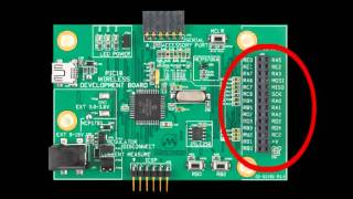
Wi-Fi Media Streaming Modules
This information applies to a product under development. Its characteristics and specifications are subject to change without notice. Roku
assumes no obligation regarding future manufacturing unless otherwise agreed to in writing. www.rokulabs.com © Roku 2005.
SPI
PAR.
I2C
Ethernet
10/100
SDRAM
16MB
Antennas
Flash
4MB
I2S
/AC97
RS232
Clocks
400MHZ
Processor
Control Header
ITU-R 656
WiFi
802.11
APPLICATIONS
Add Internet Radio, PC/MAC music library, JPEG, OSD
and music service features to:
• Music systems
• AV receivers
• TVs
• Radios
• DVD Players
FEATURES
• 3.3V RS232, I2C, Parallel, or SPI control
• Easy command protocol suitable for use by a low
cost microcontroller. Allows listing of available
internet radio stations, listing of digital music
libraries, audio playback, TCP/IP access, and
more.
• End-user web access and control
• ITU-R 656 for JPEG or OSD
• Models with built in WIFI 802.11b or 80211g, or
10/100 Auto MDIX Auto Polarity Ethernet
• WiFi drivers and certification
• Microsoft PlaysForSure certification
• Decoded Audio is output over I2S DSP style
synchronous serial port or AC97 interface
• 4Mbytes of program store, field upgradeable
• 16Mbytes of SDRAM
• Real time clock
• I2S/AC97 clock can be internal (supports
48KHz/32Khz and 44.1KHz) or externally
supplied.
• Single 3.3V power supply
• International language support
CODECS SUPPORT
• MP3, WMA, AAC
• WAV, AIFF, LPCM
• JPEG
DIGITAL RIGHTS SUPPORT
• WM DRM10
• Rhapsody
PROTOCOLS
• UPnP AV
• Apple DAAP & OpenTalk
• Rhapsody
• IP / UDP / TCP
• telnet
• SlimServer
• HTTP / HTML
• XML, SOAP
• Internet Radio (mp3, pls, m3u, asx, wma)
• Live365
• PlaysForSure
SUPPORTED SERVICES
• Rhapsody
• Napster
• MSN Music
• Walmart.com
• Musicmatch
• MusicNow
• Live365
• More…
FUNCTIONAL BLOCK DIAGRAM
MB301 / MB302 / MB303 / MB 304 Overview
Wi-Fi Media Streaming Modules
This information applies to a product under development. Its characteristics and specifications are subject to change without notice. Roku
assumes no obligation regarding future manufacturing unless otherwise agreed to in writing. www.rokulabs.com © Roku 2005.
Overview
The MB30x Wi-Fi Media Streaming Module allows the easy addition of powerful networked digital music and
display features to your product. Based on Roku’s award winning SoundBridge technology, the MB30x is a proven
and drop-in solution for adding Internet radio, music streaming, JPEG or even an On Screen Display to your
products.
By issuing commands to the streaming module over any of the control links (3.3 volt RS232, SPI, I2C, or Parallel),
you can play internet radio or digital music or stream JPEGs over a home network. The streaming module handles
the complicated work behind the scenes with its embedded and powerful Wi-Fi and network media processor.
Web Control
End users have the option of controlling and configuring the MB30x from a laptop, PC, or Mac. An icon that
represents the networked device containing the MB30x will automatically appear in the PC or Mac UI, since the
MB30x will broadcast its existence via UPnP or Rendezvous (Open Talk).
When the end-user clicks the MB30x icon, it will open a web UI for the device. From this UI, the end user can
configure options, select music to play, pause or resume play, and many other functions.
Example Operating Modes
The MB30x offers a robust control interface that allows client devices infinite control over the details of digital media
streaming, if they so desire. On the other hand, some devices may wish to add digital media support without
investing development time on a new user interface or complex operating modes. For these clients, the MB30x
provides powerful yet simple control commands that take care of all the details. The following examples show
some different usage scenarios that clients could support depending on the level of control and customization
desired:
Mode 1: Internet Radio Presets Only
In this mode, the user can only play internet radio stations. The user initiates playback by pressing a "preset
button" on the remote or front panel interface. The device μC then sends the PlayInternetRadioPreset command
to the streaming module to begin playback. The streaming module comes configured with the presets set to
popular internet radio stations, however, these can be changed using Web Control or streaming module
commands.
Mode 2: Use built-in UI
The streaming module includes a string-based user interface that supports its full range of features, including
internet radio, networked music library browsing, searching, and playback, and WiFi setup and configuration. This
UI supports displays ranging from 1 to 24 lines in height, automatically configuring its UI to the target device,
whether it has a single line VFD, a two line LCD, or is a TV with 24 lines of display space. In this mode, the
streaming module generates and sends the μC text strings to display, and then the μC displays the strings to the
user and sends user responses back the streaming module.
Mode 3: Custom UI
Your device can implement any arbitrary user interface you wish. To connect the user interface to the streaming
module, there is a rich set of control commands that allows you to browse and search all networked music libraries
and internet radio stations. Because the streaming module abstracts the complicated aspects of talking to different
server types, network drivers, protocol stacks, digital rights management and so on, you can concentrate on
building a unique UI with powerful digital music features.
Mode 4: Stand alone mode
In this mode there is no host processor. The streaming module is controlled entirely from the Ethernet or Wireless
interface using either Telnet or the built in web page.
Wi-Fi Media Streaming Modules
This information applies to a product under development. Its characteristics and specifications are subject to change without notice. Roku
assumes no obligation regarding future manufacturing unless otherwise agreed to in writing. www.rokulabs.com © Roku 2005.
Command Summary
The following are examples of the types of commands that can be issued to the MB30x via the serial port. This list
is not exhaustive.
Command Name Summary
ListServers The MB30x automatically discovers many types of music servers
on a user’s Local Area Network, such as UPnP AV (like Microsoft’s
WMC), Rhapsody, MusicMatch, iTunes, and more. This command
returns the list of currently known servers in a format suitable for
display to a user.
ListSongs There are a number of commands for browsing the content of a
music server, including ListSongs, ListAlbums, ListArtists,
ListComposers, and ListGenres. The streaming module client can
select songs, albums, artists, etc., by name or by index, and can
even browse by a combination of filters, like songs by artist in a
particular genre.
ListInternetRadioPresets The streaming module stores a list of 15 of the user’s favorite
internet radio presets for easy access, and comes pre-populated
with popular radio stations. This command returns a list of friendly
names for each preset, suitable for display to the user. The user
can change their favorites by using their web browser or by using
an streaming module command (SetInternetRadioPreset).
SearchSongs On servers that support it, the streaming module can search for
content on a music server with the commands SearchSongs,
SearchArtists, SearchAlbums, SearchComposers, and SearchAll.
GetSongInfo The streaming module client can retrieve detailed song information,
as provided by the music server, including song title, artist, album,
genre, bit rate, file format, file size, and song length.
QueueAndPlay The usual way to start music playback, QueueAndPlay creates a
playlist from the current list of browsed or searched songs and
begins playback at the specified song index.
NowPlayingQueue NowPlayingQueue allows the user to add additional songs to the
current list of playing songs. (As opposed to QueueAndPlay, which
destroys the current playlist of songs before creating a new one,
NowPlayingQueue will add additional songs to the already existing
list.)
Play All simple transport actions are available as streaming module
commands such as Play, Pause, Next, Previous, Stop, Shuffle, and
Repeat. These commands affect playback of the current Now
Playing playlist.
SubscribeTransportUpdateEvents The streaming module client can subscribe to notifications of any
change in the transport state, to give the user instant feedback.
Transport states include Paused, Playing, Buffering, Resuming,
Stopped, PlaybackError, etc.
ListWiFiNetworks Returns a list of the names (SSIDs) of wireless networks detected
by the on-board Wi-Fi adapter.
ConnectSSID Sets the wireless network (SSID) to connect to.
SetWiFiPassword Sets the password for connection to a wireless network.
GetWiFiSignalStrength Gets the real-time signal strength of the wireless network the
streaming module is currently connected to.
Wi-Fi Media Streaming Modules
This information applies to a product under development. Its characteristics and specifications are subject to change without notice. Roku
assumes no obligation regarding future manufacturing unless otherwise agreed to in writing. www.rokulabs.com © Roku 2005.
Module physical dimensions
4 inches by 2.8 inches
Pin out
30X2 2mm connector, suitable for soldering to your board connecting via a header.
pin Description pin Description
1 VCC (3.3V) 2 VCC (3.3V)
3 Ground 4 Ground
5 Ethernet TX+ 6 Ethernet TX-
7 Ground 8 Ethernet Center Tap
9 Ethernet RX+ 10 Ethernet RX-
11 Ground 12 Ground
13 IR Input (38KHz) 14 RS232 TX (3.3V)
15 RS232 RX (3.3V) 16 SPISS_L/PAR_ACK_L
17 SPI MOSI 18 SPI MISO
19 SPI CLK 20 PAR_RD_L/SPI_REQ_L
21 PAR_WR_L/SPI_ACK_L 22 ATTN_L
23 I2S/AC97 TXDATA 24 I2S/AC97 RXDATA
25 I2S/AC97 MCLK 26 I2S/AC97 BITCLK
27 External I2S/AC97 Clock 28 I2S/AC97 FRAME
29 3.3V Battery input for RTC 30 DAC_RST_L/ SPI DAC CS output
31 Ground 32 RESET_L input/output
33 VCC (3.3V) 34 VCC (3.3V)
35 LED0 (ETH 10/100) 36 PAR_D0
37 LED1 (ETH LINK/ACT) 38 PAR_D1
39 LED2 (WIFI LED1) 40 PAR_D2_PPD9
41 LED3 (WIFI LED2) 42 PAR_D3_PPD8
43 I2C_SCL 44 PAR_D4_PPD7
45 I2C_SDA 46 PAR_D5_PPD6
47 No Connect 48 PAR_D6_PPD5
49 Ground 50 PAR_D7_PPD4
51 Frame 52 PPD3
53 HSync 54 PPD2
55 VSync 56 PPD1
57 Ground 58 PPD0
59 PPCLK 60 Ground
PC/Mac Music Servers Supported:
1. Microsoft Windows Media Connect
2. Real Network’s Rhapsody
3. UPnP AV
4. Apple iTunes
5. Yahoo MusicMatch
6. WinAmp with TwonkyVision plug-in
7. SlimServer
8. mt-DAAP
Wi-Fi Media Streaming Modules
This information applies to a product under development. Its characteristics and specifications are subject to change without notice. Roku
assumes no obligation regarding future manufacturing unless otherwise agreed to in writing. www.rokulabs.com © Roku 2005.
RX/TX
RS232
IR
RJ45
IR Rec
Demod
DAC
SPDIF
I2S
/AC97
RS232
DB9
Debug
40 x 2 LCD
Front Panel
Buttons
SPI
I2C
PAR
uC
MB303
ITU-R 656
FLASH
Video
Encoder
S-VIDEO
& Comp.
ESB-EVAL Evaluation Board
The ESB-EVAL implements a complete network music player in only a few hundred lines of C code. Includes the
MB304 Network Music Module, microcontroller, LCD Display, IR receiver, and remote control. Schematics and ‘C’
source code included.
The module has been pre-screened at the FCC lab, in order to make it easier for you to get your product to market
faster.
The provided source code demonstrates the three streaming module usage modes: Mode 1: Internet Radio
Presets Only, Mode 2: Use built-in UI, and Mode 3: Custom UI.
Sales Information
For information contact: esb-sales@rokulabs.com
Part
Number
Network Type Price
100,000
per
year
Availability
MB301 Ethernet 10/100 May 05
MB302 Wi-Fi B May 05
MB303 Wi-Fi B + 10/100 May 05
MB304 Wi-Fi G June 05
MB305 Wi-Fi G + 10/100 June 05
ESB-EVAL Eval Board April 05
Revision date: 4/8/2005 4:20 PM
82-001925-01
a
ADMC401
DSP Motor Controller
Developer’s
Reference Manual
Revision 2.0
2 March 2000
ADMC401 DSP Motor Controller
Developer’s Reference Manual
Rev. 2.0 2 March 2000
82-001925-01
2
Table of Contents
1. INTRODUCTION..............................................................................................................................6
2. REFERENCED DOCUMENTS ........................................................................................................6
3. UPGRADE INFORMATION............................................................................................................7
4. GETTING STARTED .......................................................................................................................7
5. IMPORTANT SAFETY INFORMATION.......................................................................................7
6. SOFTWARE DEVELOPMENT........................................................................................................9
6.1 EVALUATION KIT SOFTWARE....................................................................................................... 11
6.2 GETTING STARTED WITH THE MOTION CONTROL DEBUGGER ........................................................ 12
6.2.1 Saving the Debugger Windows Configuration ..................................................................... 22
6.2.2 Modifying Your Program Directly From the Disassembly Window...................................... 23
6.2.3 Automatic Program Exit Function ...................................................................................... 23
6.2.4 Troubleshooting.................................................................................................................. 24
6.2.5 Error Messages .................................................................................................................. 24
6.3 PROGRAMMING SERIAL PROMS WITH MAKEPROM.................................................................... 26
6.4 USING INCLUDE FILES IN YOUR CODE........................................................................................... 27
7. ADMC401 HARDWARE OVERVIEW.......................................................................................... 28
7.1 MOTOR CONTROL PERIPHERAL REGISTERS................................................................................... 28
7.2 ADDRESS AND DATA BUS............................................................................................................. 28
8. MEMORY MAP.............................................................................................................................. 29
8.1 (MMAP = BMODE= 1 CONFIGURATION) ................................................................................... 29
8.2 (MMAP = BMODE= 0 CONFIGURATION) ................................................................................... 29
9. ON-CHIP ROM MONITOR OPERATION ................................................................................... 30
9.1 POWER-UP / RESET SEQUENCE ..................................................................................................... 30
9.2 SPORT1..................................................................................................................................... 30
9.3 THE ROM CODE MONITOR .......................................................................................................... 30
10. SOURCE CODE LIBRARY........................................................................................................ 35
11. BOOTING FROM EXTERNAL EPROM WITH MMAP=BMODE=0.................................... 36
12. INTERRUPT OPERATION........................................................................................................ 40
12.1 USING PUT_VECTOR................................................................................................................ 42
12.2 PERIPHERAL INTERRUPT CONSIDERATIONS ................................................................................... 42
13. WATCHDOG TIMER OPERATION......................................................................................... 43
14. SOFTWARE PERIPHERAL RESET FUNCTION.................................................................... 44
15. SROM/EEPROM RESET FUNCTION ...................................................................................... 44
16. TUTORIAL.................................................................................................................................. 45
16.1 EXAMPLE 1: SIMPLE CONFIGURATION EXAMPLE ........................................................................... 45
ADMC401 DSP Motor Controller
Developer’s Reference Manual
2 March 2000 Rev. 2.0
82-001925-01
3
17. APPENDICES .............................................................................................................................. 47
Figures
Figure 1. The Software Development Process .............................................................................................9
Figure 2. Debugger Target Selection Dialog Box ...................................................................................... 12
Figure 3. Debugger Disassembly Window................................................................................................. 13
Figure 4. Loading an Executable File .................................................................................................... 14
Figure 5. Using the Find Text Window ..................................................................................................... 14
Figure 6. Finding Symbols in the Program................................................................................................ 15
Figure 7. Browsing the List of Symbols .................................................................................................... 15
Figure 8. The GoTo Address Box........................................................................................................... 16
Figure 9. Selecting Breaks from the Debug Menu................................................................................. 16
Figure 10. The Breaks Dialog Box ......................................................................................................... 16
Figure 11. Running the Program............................................................................................................ 17
Figure 12. Halting and Single-Stepping ................................................................................................. 18
Figure 13. Selecting a Register from the Registers Menu ..................................................................... 18
Figure 14. Viewing the PWM Registers................................................................................................. 19
Figure 15. Viewing the Program Memory (PM).................................................................................... 19
Figure 16. Selecting Format of Data Memory ....................................................................................... 20
Figure 17. Viewing the Memory Map .................................................................................................... 20
Figure 18. Dumping Memory ................................................................................................................. 20
Figure 19. Fill Memory........................................................................................................................... 21
Figure 20. Plot Memory Configuration Dialog ...................................................................................... 21
Figure 21. Plot Memory Output ............................................................................................................. 21
Figure 22. Motion Control Debugger Version........................................................................................... 22
Figure 23. Required Timing for Interfacing to an External Device............................................................ 32
Figure 24. Monitor Operation at Reset...................................................................................................... 34
Figure 25. Watchdog Timer Register ........................................................................................................ 43
Figure 26. Boot Load Timing (XC17128E, AT17C128, or 37LV128)....................................................... 57
Figure 27. UART Protocol........................................................................................................................ 60
ADMC401 DSP Motor Controller
Developer’s Reference Manual
Rev. 2.0 2 March 2000
82-001925-01
4
Tables
Table 1. Summary of Debugger HotKeys .................................................................................................. 22
Table 2. ADMC401 Evaluation Board Memory Map (MMAP = BMODE = 1 Configuration)................... 29
Table 3. Two Byte Sequence for each Monitor Supported Interface........................................................... 31
Table 4. Interrupt Vector Addresses by Priority ........................................................................................ 40
Table 5. SROM / EEPROM Pin Connections............................................................................................ 55
Table 6. SROM boot loader error codes. ................................................................................................... 56
Table 7. File Syntax For All Boot Load Interfaces..................................................................................... 58
Table 8. Available Commands (Debugger Interface)................................................................................. 62
Table 9. Data Memory Write Command ................................................................................................... 62
Table 10. Data Memory Read Command .................................................................................................. 62
Table 11. 16-Bit Program Memory Write Command................................................................................. 62
Table 12. 16-Bit Program Memory Read Command.................................................................................. 63
Table 13. 24-Bit Program Memory Write Command................................................................................. 63
Table 14. 24-Bit Program Memory Read Command.................................................................................. 63
Table 15. Monitor Variables for Executing User Code .............................................................................. 64
Table 16. DM Write Commands to Start Program at 0x0060 .................................................................... 64
ADMC401 DSP Motor Controller
Developer’s Reference Manual
2 March 2000 Rev. 2.0
82-001925-01
5
Appendices
Appendix A. System Specification File..................................................................................................... 47
Appendix B. Architecture Description File ............................................................................................... 48
Appendix C. ADMC401 Include File (ADMC401.H) ............................................................................... 49
Appendix D. Constant Include File (Constant.h) ...................................................................................... 52
Appendix E. Macro Include File (Macro.h) .............................................................................................. 54
Appendix F. SROM/EEPROM Boot Loader Protocol................................................................................ 55
Appendix G. UART Boot Loader Protocol ................................................................................................ 59
Appendix H. UART Debugger Protocol .................................................................................................... 61
Appendix I. Synchronous Master Boot Load Protocol ............................................................................... 65
Appendix J. Synchronous Master Debugger Protocol ................................................................................ 66
Appendix K. Synchronous Slave Boot Loader Protocol ............................................................................. 67
Appendix L. Synchronous Slave Debugger Protocol ................................................................................. 68
ADMC401 DSP Motor Controller
Developer’s Reference Manual
Rev. 2.0 2 March 2000
82-001925-01
6
1. Introduction
The ADMC401 is a single chip DSP motor controller optimized for standalone motor control applications.
The device combines a 26MHz fixed point ADSP-2171 core with on-chip memory, two serial ports, a
programmable timer, and a set of on-chip motor control peripherals. In addition, the address and data bus
of the DSP core are connected to package leads allowing external memory and peripheral expansion.
Together with the list of referenced documents, this manual provides the information necessary to
understand and evaluate the processors’ architecture and to develop an ADMC401-based system.
2. Referenced Documents
Reference 1. ADMC401 Single Chip DSP Motor Controller Data Sheet, Analog Devices.
Reference 2. ADSP-2100 Family User’s Manual, Third Edition, 9/95, Analog Devices.
See “ADSP-2100 Family User’s Manual” on the Analog Devices web site at
http://www.analog.com/support/product_documentation/dsp_prdoc.html
Reference 3. ADSP-2100 Family Assembler Tools & Simulator Manual, Second Edition, 11/94,
Analog Devices.
See “ADSP-2100 Assembler Tools Manual” on the Analog Devices web site at
http://www.analog.com/support/product_documentation/dsp_prdoc.html
Reference 4. ADSP-2100 Family C Tools Manual, Second Edition, 11/94, Analog Devices.
See “ADSP-2100 C Tools Manual” on the Analog Devices web site at
http://www.analog.com/support/product_documentation/dsp_prdoc.html
Reference 5. Digital Signal Processing Applications using the ADSP-2100 Family, Volume 1,
Analog Devices, 1992.
See “Using the ADSP-2100 Family Volume 1” on the Analog Devices web site at
http://www.analog.com/support/product_documentation/dsp_prdoc.html
Reference 6 Visual DSP Debugger Guide & Reference, First Edition, July 6, 1998, Analog
Devices.
See “Visual DSP 6.0 Debugger Guide” on the Analog Devices web site at
http://www.analog.com/support/product_documentation/dsp_prdoc.html
ADMC401 DSP Motor Controller
Developer’s Reference Manual
2 March 2000 Rev. 2.0
82-001925-01
7
3. Upgrade Information
Each evaluation kit is shipped with a software version that is fully functional for basic DSP development
operations such as assembling, linking, debugging, and serial PROM formatting. This version is powerful
enough to fill the needs of most users. Those who want to use the software simulator or write C code may
add the standard development software for the ADSP-2100 Family (part number ADDS-21XX-PC-1).
NOTE: While it is possible to use the C compiler to generate code for the 2171 based motor control DSPs,
the efficiency of this code is questionable. Due to the overhead needed by the C compiler, and the memory
constraints of the 2171 based motor control DSPs, C code development is not recommended by the Motion
Control Group. The C compiler does not come with direct support for the 2171 based motor control DSPs.
In addition to the features found in the software shipped with the evaluation kit the ADSP-2100 Family
Development Software adds:
· System Builder
Define your target system hardware in an architecture description file. The linker and the simulators
use this information to know how much memory is in your system, which memory is RAM and which
is ROM, which memory is internal to the processor and which is external, and what memory-mapped
peripherals you have. You don’t need this tool since the kit software includes an architecture
description file for the ADMC401. If you need to modify the file, you can do this simply by editing the
file and following the syntax contained therein. You should not need to modify the file unless you want
to create your own memory segments.
· Simulators
Run an instruction level simulation of any ADSP-2100 Family processor. All of the ADSP-2100
Family Simulators provide an interactive, instruction-level simulation, displaying the cycle-by-cycle
operation of different portions of the processor and system hardware through a window-based graphical
user interface. NOTE: The simulators model only 21xx family general purpose DSPs. None of the
motor control peripherals are modeled.
· Librarian, C Compiler, C Runtime Library, C Debugger
The C level software tools that come with the ADSP-2100 Family development software may be used to
develop user code but it is not recommended by the Motion Control Group (see the NOTE above).
4. Getting Started
Start by reading the release notes which accompany the evaluation kit you received. They describe what is
new in the latest release and how to install the development software on the disks that accompany each
board. In addition to the software development tools, documentation and demonstration software will also
be installed. Take the time to become familiar with the documentation so that you know where to find
information when needed. Also familiarize yourself with the documents referenced by this document.
Because the ADMC401 is a combination of an ADSP-2171 DSP core and a set of motor control peripherals,
needed technical information may be located in the ADSP-2100 Family User’s Manual, the ADMC401 data
sheet, application notes, or in this document.
5. Important Safety Information
The Motion Control Debugger should be used in a live system only with extreme caution. Your software
should first be developed with an ADMC401 evaluation kit or target board that is not connected to a motor.
ADMC401 DSP Motor Controller
Developer’s Reference Manual
Rev. 2.0 2 March 2000
82-001925-01
8
WARNING: PWM SIGNALS TO THE MOTOR REMAIN ACTIVE AT A BREAKPOINT!
If you want the motor shut down then use the HALT function to stop your program from executing. The
halt function performs a peripheral reset when halting your program. The halt function is executed by
selecting Halt from the Debug menu or by clicking the Halt button . DO NOT use breakpoints with a
live system because the PWM stage will remain active.
ADMC401 DSP Motor Controller
Developer’s Reference Manual
2 March 2000 Rev. 2.0
82-001925-01
9
6. Software Development
Figure 1 shows the software development process that a user will follow to create an ADMC401 application.
The software tools used, shown in boxes in Figure 1, run on an IBM compatible PC. The System Builder,
Assembler, Linker, C Compiler, and PROM splitter, and MAKEPROM utility must be run in a DOS
window. The Motion Control Debugger and Simulator are invoked from Windows 95 or Windows NT.
Although ADMC401 specific information is contained in this document, the basic tool operations are
discussed in the references. The System Builder, Assembler, Linker, and PROM splitter are discussed in
Reference 3. The C Compiler is discussed in Reference 4. The Simulators are discussed in Reference 6. The
Motion Control Debugger is discussed in this document and in the latest version of its release notes. The
MAKEPROM utility is discussed in this document. The tools shown as optional are not needed by most
users and, therefore, are not included in the ADMC401 evaluation kit. They can be acquired by ordering
the standard development software for the ADSP-2100 Family (part number ADDS-21XX-PC-1). The
operation of this optional software is described in Italic font.
System
Architecture
File
System
Specification
File
System
Builder
C Source
Files
Linker
ANSI
C Compiler
Libraries
Executable
File
Assembler
Assembler
Source
Files
STEP 1:
Describe
Architecture
STEP 2:
Generate
Code
Software Simulator
ADMCxxx
Evaluation
Board
Motion Control
Debugger
Target Board
MAKEPROM
(SROM or EEPROM)
Motion Control
Debugger
STEP 3:
Debug
Software
STEP 4:
Final
Version for
Production
User File or Hardware Software Development Tool Hardware Development Tool
Optional Software Development Tool
PROM Splitter
Figure 1. The Software Development Process
ADMC401 DSP Motor Controller
Developer’s Reference Manual
Rev. 2.0 2 March 2000
82-001925-01
10
(Optional software) The software development process begins with the task of defining the target system
architecture. To do this you use the system builder. You must write a system specification file as input to
the system builder; this file describes the target hardware configuration and memory map. The system
builder reads the file and generates an architecture description file which passes this information to the
linker and simulator.
The above step may be skipped if you choose to use the ADMC401 architecture description file that is
installed when the development software is installed. The system specification file that was used to create
this architecture description file is also installed and can be used as a starting point for your own target
hardware. These files are also available in Appendix A and Appendix B. If you do not have the system
builder tool and wish to make a change to the .ach file you can edit it since it is a text file. Just mimic the
syntax observable within the file.
You begin code generation by creating assembly language source code modules. An assembly code module
is a unit of assembly language comprising a main program, subroutine, or data variable declarations.
Include files are provided in the appendices that contain things like ADMC401 specific constants and
macros that can be used in your code. These files can be included in source routines to provide a simple
interface to the ADMC401’s motor peripheral registers, and interrupt vector table addresses. These files are
also installed along with the development software and used in the tutorial given in this document. They
can be found in the main installation directory in a subdirectory called TgtFiles.
(Optional software) Each code module is assembled separately by the assembler into ADSP-2171 machine
code. Alternatively, the C compiler can be used to generate machine code from C source code.
The linker reads the target hardware information from the architecture description file to determine
placement of code and data fragments. In the assembly modules you may specify each code/data fragment
as completely relocatable, relocatable within a defined memory segment, or non-relocatable (placed at an
absolute address). Non-relocatable code or data modules are placed at the specified memory address,
provided the memory area has the correct attributes. Relocatable objects are placed in memory by the
linker.
Using the architecture description file and assembled code modules, the linker determines the placement of
relocatable code and data modules, and places all modules in memory locations with the correct attributes
(CODE or DATA, RAM or ROM). The linker generates a memory image file containing a single
executable program which may be loaded into a simulator, or downloaded to the evaluation kit or target
hardware, using the Motion Control Debugger, for testing.
(Optional software) The simulator provides windows that display different portions of the hardware
environment. To replicate the target hardware, the simulator configures its memory according to the
architecture description file. To simulate ADMC401 code you must use the ADSP-2101 simulator because
the ADSP-2171 simulator does not support the memory map of the ADMC401. ADMC401 peripherals are
not supported on any of the ADSP-21XX family simulators. You can configure the peripheral registers as
I/O ports on the simulator to verify that you are initializing them correctly, but you can’t view the
operation of the peripherals. For this reason it is recommended that you use the simulator only for basic
DSP core programming issues and that you use the ADMC401 evaluation kit with the Motion Control
Debugger for true application development.
The Motion Control Debugger allows you to download your executable file to an ADMC401 processor
board or your own target hardware, to debug your code, and to test your application directly over a standard
UART interface. Similar to the simulators, the debugger displays the hardware environment of the
ADMC401 through a series of windows. However, with the debugger you have full access to all of the
registers and memory on the ADMC401.
ADMC401 DSP Motor Controller
Developer’s Reference Manual
2 March 2000 Rev. 2.0
82-001925-01
11
As Figure 1 shows, the software development process is an iterative one as you continue to debug and add to
your application code. Once your code is stable you have the option of programming a serial ROM or
EEPROM, or a byte-wide EPROM so that your code is boot loaded automatically to the ADMC401 on
power-up or reset.
The serial ROM boot load interface is provided by the on-chip ROM monitor program. To use this interface
you must format your executable file using the MAKEPROM utility which takes your executable file and
converts it into a PROM programmer compatible file that has the correct boot loader protocol. Use of the
MAKEPROM utility is discussed later in this document.
The byte-wide EPROM method of booting takes advantage of the built in boot memory interface of the
ADMC401 core. This interface is available when the BMODE and MMAP pins are tied low. To use this
interface you must format your executable file using the PROM splitter tool. Use of the PROM splitter is
discussed later in this document.
In addition to the methods of booting described above you also have the option of booting from an external
UART. This interface is also provided by the on-chip ROM monitor and is discussed later in this
document.
6.1 Evaluation Kit Software
If you have any older versions of the Motion Control Development Tools installed on your computer, you
must fully uninstall them before installing this version.
If you have any older versions of the Analog Devices 16 bit DSP development tools, such as ADSP 21XX,
or VDSP, it is strongly recommended that you upgrade to the latest VisualDSP tool set before installing the
Motion Control Development Tools.
Whether you are installing from CD-ROM or downloading from the WEB, the executable file,
SETUP.EXE, will install the development tools, applications notes, developer’s reference manual, and
example software onto your computer. You will be prompted for instructions during the installation.
If asked whether you want to install the 16 bit DSP tools, you should answer YES only if you have NOT
already installed some version of the Analog Devices 16 bit DSP development tools, such as VisualDSP.
If you answer YES, a subset of these tools (assembler, linker, librarian, and prom splitter) will be installed
onto your computer. If you already have these tools on your computer, then you should answer NO to this
prompt.
When prompted to select targets, select the ADMC401 and any other targets that you are installing at this
time.
After installation you will have a directory structure, similar to the following, added to your PC. This
example shows what the directory structure looks like if you choose the default directories.
Drive:\Program Files\Analog Devices\Motion Control Development Tools Main installation directory
The following subdirectories are contained in the main installation directory.
Documentation\ReleaseNotes Release notes (if applicable)
Documentation\ReferenceManuals Developer's reference and user manuals
Documentation\ApplicationNotes Application notes (if applicable)
Documentation\DataSheets Data sheets
Examples Demonstration/Evaluation software
Bin Debugger executables
TgtFiles Target specific files (.h, .ach,.sys)
SrcLib Source code for library functions
WindowFiles Saved windows configurations
Uninstall.isu Used to uninstall software
ADMC401 DSP Motor Controller
Developer’s Reference Manual
Rev. 2.0 2 March 2000
82-001925-01
12
21XX\Makeprom.exe Makeprom utility program
If you install the 16 bit tools, the files listed below will have been installed. In addition, your autoexec.bat
file will have been updated so that your PATH variable includes the directory: Drive:\Program
Files\AnalogDevices\Motion Control Debugger\21XX\
21XX\Spl21.exe ADSP-21XX Family Splitter
21XX\Asm21.exe ADSP-21XX Family Assembler
21XX\Ld21.exe ADSP-21XX Family Linker
21XX\Asmpp.exe ADSP-21XX Family Pre-Processor
21XX\Asm2.exe ADSP-21XX Family Assembler Driver
21XX\Lib21.exe ADSP-21XX Family Librarian
NOTE: For more example software and the latest documentation always consult the Analog Devices Motor
Control website at http://www.analog.com/motorcontrol
6.2 Getting Started with the Motion Control Debugger
The following steps will help you get started using the Motion Control Debugger. They can be performed
alone, or in conjunction with the tutorial in section 16.
The Debugger provides a toolbar, a menu, and several shortcut keys. Many of the steps listed below
describe two or three different ways of doing the same thing. This is not meant to confuse, but to allow you
to choose the method with which you are most accustomed.
Install the Motion Control Development Tools. Refer to the release notes that came with the installation
CD.
Connect the ADMC401 board to a communication port on your computer using a standard 9 pin male-tofemale
serial cable.
Apply power to the target board, and press the hardware-reset button.
Run the Debugger. To start the debugger under Windows 95/NT select it from the start menu (Programs->
ADI Motion Control -> Debugger). The Target Selection Dialog Box (Figure 2) will appear, displaying
default values for the communications port, baud rate, clock (crystal) frequency, target, and platform.
Figure 2. Debugger Target Selection Dialog Box
Create New Platform
Delete Platform
Platform
Name
ADMC401 DSP Motor Controller
Developer’s Reference Manual
2 March 2000 Rev. 2.0
82-001925-01
13
Select a Target. Use the Debug_Target field to select the Debug Target that you wish to communicate
with. The Platform field enables you to save multiple configurations for the same target, by defining new
platforms, in case you have more than one evaluation board for the same chip. Select the COMM PORT
that is connected to the processor board, and select the desired BAUD RATE for the port. Select the
appropriate CLKIN RATE, and click OK. If you select CANCEL, you will exit the Debugger.
Attach to the Target. The Debugger will now attempt to attach to the target using the parameters you have
selected. When the Debugger has successfully attached to the target, the disassembly window (shown
below) will appear with the start location at 0x0060 highlighted. This is the point at which user code will
begin execution when a run or single step command is executed, so the beginning of your program must be
linked at 0x0060. You now have full emulation capability of your target design.
Figure 3. Debugger Disassembly Window
The greater-than sign (>) next to the address field of a code line represents the processor’s program counter
(PC) register. The program counter (PC) register points to the instruction that the processor is going to
execute next.
The processor status is shown at the bottom of the main window. The processor is currently in the state
“Reset”.
Program Counter
Processor Status
ADMC401 DSP Motor Controller
Developer’s Reference Manual
Rev. 2.0 2 March 2000
82-001925-01
14
Load a Program. A DSP program
may consist of program memory (PM)
blocks, data memory (DM) blocks, and
flash program memory (FM) blocks.
To load a program containing these
block types, select Load Program from
the File menu and navigate to the
directory containing your executable
file (.exe). Double click the desired
executable program and the debugger
will load the PM Blocks, DM Blocks,
and symbols.
Figure 4. Loading an Executable File
View the User Program. To view the program, use the page up, page down, up arrow, and down arrow
keys in the disassembly window. If the disassembly window hides behind another window, you can bring it
to the front by selecting Disassembly from the Window menu, or by clicking the Disassembly Window button
. To go back to displaying the current program counter (PC) address, press the F12 key.
Search for a Symbol. To find the line of
code where a symbol is defined, select
Find from the Search menu, or press Ctrl-
F, or click the Find button , and then
enter the symbol name.
Figure 5. Using the Find Text Window
ADMC401 DSP Motor Controller
Developer’s Reference Manual
2 March 2000 Rev. 2.0
82-001925-01
15
The disassembly window will display the code where that symbol is defined or referenced, without
modifying the program counter (PC) register. To find the next occurrence of the symbol, select Find
Again from the Search menu, or press the F3 key, or click the Find Again button .
Go To a Symbol. To select from the list of all
symbols, and display the code where that symbol is
defined or referenced, select Go To from the Search
menu, or press Ctrl-G, or click the Go To button
, and then click the Browse button. Select the
symbol from the list displayed. The disassembly
window will display the code where that symbol is
defined or referenced without modifying the
program counter (PC) register.
Figure 6. Finding Symbols in the Program
Figure 7. Browsing the List of Symbols
ADMC401 DSP Motor Controller
Developer’s Reference Manual
Rev. 2.0 2 March 2000
82-001925-01
16
Go To an Address. To display the code at a particular
address, select Go To from the Search menu, or press
Ctrl-G, or click the Go To button , and then enter the
desired address. Hexadecimal numbers must be prefixed
with “0x”, and octal numbers with “0”. Decimal
numbers must be entered starting with the most
significant non-zero digit.
Display Additional Files.
To display a file in its own
window, select Open from
the File menu or click the
Open button , and then
navigate to the desired file.
Set a Breakpoint. To set a
breakpoint, select Breaks
from the Debug menu and
add the desired line of code
to the list displayed, or
click the Break button
while the desired line of
code is highlighted. If you
prefer a shortcut method,
double click the desired
line of code, or move the
cursor to the line and press
the F9 key.
Clear a Breakpoint. To clear a break point, select
Breaks from the Debug menu. Either delete the
desired line of code from the list, or click the Toggle
Break button with the line of code highlighted. If
you prefer a shortcut method, either double click the
line of code where the break point is set, or move
the cursor to the line and press the F9 key.
Clear All Breakpoints. To clear all break points,
select Breaks from the Debug menu and then select
Clear All and OK, or simply click the Clear Breaks
button .
Figure 8. The GoTo Address Box
Figure 9. Selecting Breaks from the Debug Menu
Figure 10. The Breaks Dialog Box
ADMC401 DSP Motor Controller
Developer’s Reference Manual
2 March 2000 Rev. 2.0
82-001925-01
17
Run the Program. To run
your program, select Run from
the Debug menu, or press the
F5 key, or click on the Run
button . Observe the
processor status at the bottom
of the main window change
from “Reset” to “Running”.
WARNING! PWM SIGNALS TO THE MOTOR REMAIN ACTIVE AT A BREAKPOINT! If you want
the motor shut down then use the HALT function to stop your program from executing. The HALT function
performs a peripheral reset when halting your program. The HALT function is executed by selecting Halt
from the Debug menu or by clicking the Halt button . DO NOT use breakpoints with a live system, as
the PWM stage will remain active.
Figure 11. Running the Program
ADMC401 DSP Motor Controller
Developer’s Reference Manual
Rev. 2.0 2 March 2000
82-001925-01
18
Halt the Program. To halt a program while it is running, select Halt from the Debug menu, or press the F6
key, or click the Halt button . Observe the processor status at the bottom of the main window change
from “Running” to “Halted”. The disassembly window will display the location at which your code halted.
The greater-than sign signifies the location in the program counter (PC) register.
Single Step. To single step through your code, select Step Into from the Debug menu, or press the F11 key,
or click on the Single Step button . Observe the processor status change from “Halted” to “Stepping” to
“Halted” again.
Figure 12. Halting and Single-Stepping
Figure 13. Selecting a Register from the Registers Menu
ADMC401 DSP Motor Controller
Developer’s Reference Manual
2 March 2000 Rev. 2.0
82-001925-01
19
View Registers. To view register values while debugging your code, select them from the Register
menu. Register values are updated each time the program is halted or a breakpoint is reached. Stacks
are also selected from the Register menu. Figure 14 shows an example of viewing the PWM registers.
For a more customized register
window, select Custom from the
Register menu. This allows you to
select the specific registers you
want to view and places them all in
the same window. Some targetspecific
registers are available only
from Custom selection.
View Memory. Viewing of
program or data memory
can be selected from the
Memory menu.
Clicking the right mouse
button while the cursor is in
a memory window will
bring up a menu that allows
you to change the format of
the data displayed. Figure
16 shows data memory
displayed in fractional
format, as the user is
selecting hexadecimal
format.
Figure 14. Viewing the PWM Registers
Figure 15. Viewing the Program Memory (PM)
ADMC401 DSP Motor Controller
Developer’s Reference Manual
Rev. 2.0 2 March 2000
82-001925-01
20
You can also select
tracking from this menu.
This allows you to track
the data pointed to by a
DAG or PC register.
View Memory Map. To see the memory map for the
target you are running select Memory Map from the
Memory menu.
Dump Memory. To dump memory to the output
window or to a file, select Dump from the Memory
menu and fill in the dialog box.
Figure 16. Selecting Format of Data Memory
Figure 17. Viewing the Memory Map
Figure 18. Dumping Memory
ADMC401 DSP Motor Controller
Developer’s Reference Manual
2 March 2000 Rev. 2.0
82-001925-01
21
Fill Memory. To fill memory with a specified value,
select Fill from the Memory menu and fill in the dialog
box. Memory can also be filled from a file.
Plot Memory. To plot memory, select Plot from
the Memory menu and fill in the dialog box. The
plot will be displayed in its own window. Clicking
the right mouse button while the cursor is in a plot
window will bring up a menu that allows you to
configure the plot in different ways.
Software Reset. To execute a soft reset of the
processor, select Reset from the Debug menu, or
press the F7 key, or click the Reset button .
Observe the processor status change to “Reset”.
Restart. To restart your program,
select Reset from the Debug menu
and then Run.
Reload. To reload the most
recently loaded executable file,
select it from the most recently
loaded list found on the File menu.
Alternatively, you can press the F4
key. There are up to 4 files listed
on the most recently loaded list.
Pressing the F4 key will always
load the first file on that list.
Figure 19. Fill Memory
Figure 20. Plot Memory Configuration Dialog
Figure 21. Plot Memory Output
ADMC401 DSP Motor Controller
Developer’s Reference Manual
Rev. 2.0 2 March 2000
82-001925-01
22
Display Version. To display which version of the
Motion Control Debugger you have installed, select
About Debugger from the Help menu, or click the About
button .
Exit the Debugger. To exit the debugger, select Exit
from the File menu, or press the Ctrl-E key
combination.
NOTE: The reset and halt functions perform a peripheral reset which puts the peripheral blocks in their
power-up state (disabled). Loading an executable file will also perform a peripheral reset.
HotKey Function
F3 Find again
F4 Reload most recently loaded program
F5 Run
F6 Halt
F7 Software reset
F9 Toggle breakpoint
F11 Single step
F12 Update all windows
Ctrl-L Load program
Ctrl-O Open file
Ctrl-E Exit debugger
Ctrl-F Find
Ctrl-G Goto address or symbol
Table 1. Summary of Debugger HotKeys
6.2.1 Saving the Debugger Windows Configuration
The debugger will automatically save the current configuration of all open windows before it exits. The
next time you start the debugger the windows will be restored to the way you last left them. In addition, it is
possible to save multiple window configurations. For example, you could have one configuration that you
use to debug the PWM portion of your application, and another that you use to debug the ADC portion.
The debugger saves the windows configuration in a motion control window (.mcw) file. The default file
used is “default.mcw”. All window configuration files are saved in the WindowFiles directory found in the
main installation directory. To force a save of the current windows configuration select SaveWindows from
the File menu. The current windows configuration will be saved to the currently selected file. To save to a
different file select SaveWindowsAs from the File menu. This will change the currently selected file to this
new file you’ve chosen and then save the configuration. You can save multiple window configuration files
in the WindowFiles directory. To load a previously saved window configuration file select LoadWindows
from the File menu. The filename for the currently selected window configuration is saved in the registry
so it can be reloaded the next time the debugger is started.
Figure 22. Motion Control Debugger Version
ADMC401 DSP Motor Controller
Developer’s Reference Manual
2 March 2000 Rev. 2.0
82-001925-01
23
NOTE: Do not remove or edit the currently selected .mcw file in the WindowFiles directory. If you do the
debugger might crash or you might receive a warning that the windows configuration file cannot be opened.
If this happens you must reinstall the debugger software. This will restore the default.mcw file.
Motion Control Windows files (.mcw) are not portable between versions of the debugger software. If you
upgrade to a new version of the debugger software you must recreate your windows configuration. Because
of this requirement the debugger software installation script will delete all .mcw files from the WindowFiles
directory and copy in the new default.mcw file.
6.2.2 Modifying Your Program Directly From the Disassembly Window
The disassembly window shows the contents of program memory in disassembled format. When you load
your program executable (.exe) file you will see it displayed in the disassembly window. The standard
method of changing your program is to edit the original source code and then assemble, link, and reload the
file with the debugger.
Alternatively, you can modify your program by typing assembly language directly into the disassembly
window. This can be extremely helpful for making quick changes while testing. For example, if you are
trying to find the correct value for a delay loop it is much quicker and easier to enter the new constant
directly into your program in the disassembly window and rerun the program rather than to recompile and
reload your code each time you want to try a new value. Once the correct value has been determined you
can enter it into your source code file. As another example, suppose you suspect a certain line of code
might be causing a bug in your program. You can quickly modify that line of code or enter a NOP in that
location and rerun the program. To reverse the changes you made simply reload your executable file using
the F4 key.
Remember that any changes you make in the disassembly window will be lost if you reset or power down
the processor, or if you load another program. It’s a good idea to keep your source files up to date with any
changes you want to keep. For a quick record of the changes you have made you can dump program
memory to a file. Select Assembly as the format and the file will contain the code in disassembled format
similar to the disassembly window.
When typing in the disassembly window you can use any symbols that are currently loaded. This means
you can call routines and load variables by name rather than address. You can also refer to any of the
memory mapped peripheral registers by name. You cannot refer to symbols directly until you have loaded a
program because that’s when the internal symbol table used by the debugger is created.
6.2.3 Automatic Program Exit Function
Typically, when the debugger runs a user’s DSP program the only way to pass control back to the debugger
is by hitting a breakpoint or by executing a Halt from the debugger. The user usually creates an infinite
loop in the program so that the DSP will continue to run until the Halt is executed.
As another option, you may insert an automatic exit back to the debugger by jumping to the Exit library
function. Exit.dsp performs the same DSP functions as the debugger’s Halt function so it’s effect is to
return control back to the debugger automatically when the user’s program has finished. You will see the
debugger halt when this happens. If you try to continue running the program it will just return back to the
debugger immediately. You can execute a reset or reload the program to run it again. To use the Exit
function, assemble and link the exit.dsp file (found in the SrcLib directory) with your code. You can then
insert a JUMP EXIT wherever you wish the program to return to the debugger.
ADMC401 DSP Motor Controller
Developer’s Reference Manual
Rev. 2.0 2 March 2000
82-001925-01
24
6.2.4 Troubleshooting
The following is a list of remedies to problems you may encounter when using the Motion Control
Debugger.
a. If the debugger is not responding, your target could be in run mode. Try selecting Halt from the
Debug pulldown menu.
b. If the debugger is hung, try resetting the target board. If the debugger is not responding, invoke the
‘Close Program’ dialog box by pressing Alt-Ctrl-Delete, select Debugapp, and click ‘End Task’.
Also, End any tasks called “Motion Control Debugger”. Next press Reset on the target board and
restart the debugger.
c. If the debugger hangs, you could be writing to a part of data memory that is being used by the
debugger. See the ADMC401 memory map in this document which shows the data memory
locations that are reserved by the monitor and make sure you are not using that memory. If you
created a .map file with the -x option when you linked your program, it will show you where your
program resides in memory.
d. The debugger uses the SPORT1 transmit and receive interrupts. Keep them enabled in your code
and do not modify the corresponding interrupt vectors at locations 0x0020 and 0x0024. Failure to
do this can cause the debugger to hang.
e. The debugger also uses locations 0x0001 and 0x0002 in the interrupt vector table. Do not modify
these locations, or the debugger will hang.
f. If the debugger frequently hangs, and your PC is located in an electrically noisy environment, try
lowering the baud rate. This can be done in the Target Selection Dialog Box, when you first start
the Debugger. Lowering the baud rate will slow down the debugger, but may alleviate the
problem.
6.2.5 Error Messages
The following is a list of error messages that may be encountered while running the debugger. Following
each error message is an explanation for the error and possible steps to take to correct the problem. If the
problem can not be fixed contact the Motion Control Group for help.
ERROR_MCG0001:: Com line status change or power failure
The debugger has detected a change in the serial communications. Exit the debugger. If the
debugger is not responding, invoke the ‘Close Program’ dialog box by pressing Alt-Ctrl-Delete,
select Debugapp, and click ‘End Task’. Reset the board, and then restart the debugger.
ERROR_MCG0002:: Target communication not established
The debugger is unable to communicate with the ROM Monitor Program. Exit the debugger. If
the debugger is not responding, invoke the ‘Close Program’ dialog box by pressing Alt-Ctrl-Delete,
select Debugapp, and click ‘End Task’. Check all connections, reset the board, and then restart the
debugger. If you have the debugger installed for multiple targets make sure you are running the
correct one. Also, make sure the clock frequency for the board is correct. The clock frequency is
displayed in the target selection box when you start the Motion Control Debugger.
ERROR_MCG0003:: Serial line status error. Check continuity of serial cable and connections.
The wrong com port could be connected to the target. The serial cable could be unconnected or
broken. A board connector could be broken. Exit the debugger. If the debugger is not responding,
invoke the ‘Close Program’ dialog box by pressing Alt-Ctrl-Delete, select Debugapp, and click
ADMC401 DSP Motor Controller
Developer’s Reference Manual
2 March 2000 Rev. 2.0
82-001925-01
25
‘End Task’. Verify the connection, reconnect or fix the serial line and reset the board. Re-run the
debugger and verify the comm port selections in the target selection box.
ERROR_MCG0004:: Unable to open com port
The com port is being used by another application, or by a previous debugger session that hasn’t
`terminated properly. Exit all other applications that might be using the com port. Exit the
debugger. If the debugger is not responding, invoke the ‘Close Program’ dialog box by pressing
Alt-Ctrl-Delete, select Debugapp, and click ‘End Task’. If there are other occurrences of
Debugapp, exit them the same way. End any tasks with the name “Debugapp” or “…Motion
Control Debugger…”. Reset the board then restart the debugger.
ERROR_MCG0005:: Registry parameters not found
The registry has been corrupted. Uninstall, then Reinstall the development software on your PC.
ERROR_MCG0006:: Failed to open registry
The registry has been corrupted. Uninstall, then Reinstall the development software on your PC.
ERROR_MCG0007:: Detected a board reset or power failure.
You have performed a H/W reset of the board, or there was a power failure, while the debugger
was running. Acknowledge the error windows that pop up, then select Reset from the debug menu.
If the debugger is not responding, invoke the ‘Close Program’ dialog box by pressing Alt-Ctrl-
Delete, select Debugapp, and click ‘End Task’. Reset the board, then restart the debugger.
ERROR_MCG0008:: Error loading the monitor tasks
The development software might be corrupted. Try reinstalling the software on your PC.
ERROR_MCG0009:: Invalid target response
The debugger can’t reconnect with the ROM Monitor Program after running a user program.
Make sure you have the SPORT1 interrupts enabled in your code, you do not corrupt the SPORT1
interrupt vectors, and you do not corrupt any of the SPORT1 configuration registers.
ERROR_MCG0010:: Unable to read target memory while target is running
You’ve tried to access memory while your program is running. Halt the program and try again.
ERROR_MCG0011:: Unable to write to target memory while target is running
You’ve tried to access memory while your program is running. Halt the program and try again.
ERROR_MCG0012:: Unable to find the DSP monitor task files
The files might be corrupted. Reinstall the development software on your PC.
ERROR_MCG0013:: Target is running
Cannot perform operation while the target is running. Halt the target first.
ERROR_MCG0014:: Target communication not established after reset
The debugger is unable to communicate with the ROM monitor program. Exit the debugger. If
the debugger is not responding, invoke the ‘Close Program’ dialog box by pressing Alt-Ctrl-Delete,
select Debugapp, and click ‘End Task’. Reset the board, and then restart the debugger. If you
have the debugger installed for multiple targets make sure you are running the correct one.
ERROR_MCG0015:: Target communication Failure
The debugger is unable to communicate with the ROM Monitor Program using the parameters
specified in the target selection box which appears when you start the debugger.. Exit the
debugger. If the debugger is not responding, invoke the ‘Close Program’ dialog box by pressing
Alt-Ctrl-Delete, select Debugapp, and click ‘End Task’. Reset the board, and then restart the
ADMC401 DSP Motor Controller
Developer’s Reference Manual
Rev. 2.0 2 March 2000
82-001925-01
26
debugger. If the problem persists it could be due to noise or a hardware fault. Try lowering the
baud rate in the target selection box, which appears when you start the debugger.
ERROR_MCG0016:: Communications Failure.
The debugger cannot communicate with the target board. The most common cause of this is
failure to press the hardware reset button, or to cycle power on the target before starting the
debugger. Each time you start the debugger you must first reset the target. If you get an
“ERROR_MCG0003:: Serial line status error” prior to this error, then there is a problem with the
com port connection. The serial cable might be disconnected or you might be configured for the
wrong com port. Verify the communication parameters in the target selection box which appears
when you start the debugger.. Also, check the serial cable connection. This error can also occur if
the SPORT1 interrupts become unmasked in the IMASK register or if the SPORT1 interrupt
vectors at locations 0x20 and 0x24 are destroyed (for example if you load something at these
locations). This error can also occur if you accidentally reset the target while the debugger is
running. Another possible cause is noise on the serial line, which can happen when you run the
debugger in a fully loaded motor application.
The debugger can sometimes recover from this error. Try pressing the h/w reset button and then
clicking Retry. This combination may have to be performed several times to recover. If the
debugger is not responding, invoke the ‘Close Program’ dialog box by pressing Alt-Ctrl-Delete,
select Debugapp, and click ‘End Task’. Reset the target, and then restart the debugger.
ERROR_MCG0017:: The target never acknowledged the halt!
Possibly the SPORT1 interrupts were disabled by the user program.
When you issue a halt command to the debugger (click the Halt button), the debugger sends a halt
command to the target over the SPORT1 serial connection. In order for the target to receive this
command, the SPORT1 interrupts must be enabled and the SPORT1 received interrupt must be
serviced. Possibly your program masked the SPORT1 interrupts in the IMASK register. This is a
common problem. To run with the debugger your program must keep the SPORT1 interrupts
unmasked in the IMASK register (IMASK=6) and keep the SPORT1 interrupt vectors at locations
0x20 and 0x24 uncorrupted. If your program spends a lot of time in interrupt service routines, you
should add the line “IMASK=6” at the top of your interrupt service routine. This will override the
automatic setting of IMASK=0 that is done when a non-nested interrupt is serviced. This will
allow the debugger to halt the target in an interrupt service routine. Another possible cause of this
error may occur if your program spends so much time in higher priority interrupt service routines
that the SPORT1 receive interrupt is never serviced.
6.3 Programming Serial PROMs with MAKEPROM
By using the Makeprom utility and a standard PROM programmer, a user’s code may be programmed into
a serial PROM for boot loading the ADMC401 at reset. The Makeprom utility will convert an executable
file (.EXE) into a binary file (.DBS) for use with the PROM programmer. The binary file created is
automatically formatted to work with the boot loader of the ADMC401. The boot loading protocol is
compatible with the Xilinx XC17128E SROM, the Atmel AT17C128 EEPROM, and the Microchip
37LV128 EPROM. The Makeprom Utility (MAKEPROM.EXE) is installed with the Motion Control
Development Tools software. It runs from an MS-DOS window similar to the other development tools.
Follow these steps to create a serial device containing your executable image:
1. Your executable code must be linked to start executing at the beginning of user program memory
(0x0060), to which the boot loader will jump after loading the executable program. Consequently, you
are required to have a minimum of 1 block of code linked into program memory for the boot loader to
succeed. You are not required to have data linked into data memory. However, if this is the case, the
boot loader will automatically write 4 zeros at the start of data memory (0x3800). NOTE: Do not try
loading the interrupt vector table during a boot load. This would overwrite the default interrupt vector
ADMC401 DSP Motor Controller
Developer’s Reference Manual
2 March 2000 Rev. 2.0
82-001925-01
27
table, which is needed by the boot loader. Instead you should modify the interrupt vector table from
within your program by using the library routine PUT_VECTOR. (See the putvctr.dsp file in the
SrcLib directory.
2. Run Makeprom which has the following syntax:
usage: Makeprom -i -t [-o ] [-c]
-i Input file
-t Target (e.g. ADMC401)
-o Output file (default = input_file.dbs)
-c Display checksums
-x Create text file. (default = binary)
-h Header disable. Suppresses SROM/EEPROM header
-m Mirror image disable. Data will be MSB…LSB.
3. Load the output file into your PROM programmer and select one of the devices listed above. The data
format of the file is absolute binary. NOTE: Make sure the polarity option is set to program an active
low reset ( RESET /OE).
4. Program the device and place it in the SROM/EEPROM socket of the processor or target board.
5. On power-up or reset, your executable code will be loaded at the start of user memory and executed.
6.4 Using Include Files in Your Code
Include files are useful for reusing code and data items that are shared between programs without having to
duplicate them in each program. The ADMC401 development software contains a number of include files
which can be used throughout your code. For example, the ADMC401.h file contains constants set equal to
the memory-mapped registers and interrupt vector table addresses. If you include this file you can refer to
the ADMC401 registers and interrupt vector table locations by name instead of by address. The code
snippet below illustrates how to use the ADMC401.h include file for setting up the PWMSYNC interrupt
vector table entry. PWMSYNC_INT_ADDR and PUT_VECTOR are constants defined in ADMC401.h.
#include ;
Initialize_Interrupts:
I4 = PWMSYNC_INT_ADDR;
MR0 = ^YOUR_PWMSYNC_ISR
CALL PUT_VECTOR;
IMPORTANT: The last line of an include file must contain a carriage return or subsequent include
statements will be ignored. Also, always use the #include directive instead of the .INCLUDE directive.
#include allows you to put precompiler directives in your include files while .INCLUDE doesn’t.
ADMC401 DSP Motor Controller
Developer’s Reference Manual
Rev. 2.0 2 March 2000
82-001925-01
28
7. ADMC401 Hardware Overview
The ADMC401 uses several ADSP-21XX family resources including: an ADSP-2171 core, 2K of on-chip
program RAM, 2K of on-chip program ROM, 1K of on-chip data RAM, two serial ports, and a
programmable timer. The operation of each of these units is described fully in Reference 2.
7.1 Motor Control Peripheral Registers
In addition to the ADSP-2171 core peripherals, the ADMC401 contains a set of motor control peripherals
that are controlled through registers that are memory-mapped into the core’s data memory. The operation
of the peripherals is described in Reference 1.
7.2 Address and Data Bus
The ADMC401 provides the 14-bit address bus and 24-bit data bus on external pins for memory and
peripheral expansion. See Reference 1 for details about this capability.
ADMC401 DSP Motor Controller
Developer’s Reference Manual
2 March 2000 Rev. 2.0
82-001925-01
29
8. Memory Map
8.1 (MMAP = BMODE= 1 Configuration)
The following table shows the memory map for the ADMC401 evaluation board when the MMAP and
BMODE pins are both connected to a logic 1. This is the mode that enables the ROM monitor Programs
and thus allows use of the Motion Control Debugger, as well as programs to be boot loaded from serial
ROM or EEPROM. If you are booting the ADMC401 in any other mode other than MMAP = BMODE =
1, consult References 1 and 2 for proper operation.
There are a few memory restrictions when using the evaluation board in the MMAP = BMODE = 1
configuration. For proper operation of the Motion Control Debugger and SROM boot loader, never link
programs into the Data Memory RAM locations marked “Reserved by Monitor”. In addition, the debugger
uses locations 0x0001, 0x0002, 0x0020, and 0x0024 of the interrupt vector table. Do not modify these
locations when running with the debugger.
Program Memory
Address Range Memory Type Function
0x0000 - 0x005F Internal RAM Interrupt Vector Table
0x0060 - 0x07FF Internal RAM User Program Space
0x0800 - 0x0FFF ROM Monitor
0x1000 - 0x3FFF External RAM User Program Space
Data Memory
Address Range Memory Type Function
0x0000 - 0x1FFF External RAM User Data Space
0x2000 - 0x23FF Memory Mapped Peripheral Registers
0x2400 - 0x37FF External RAM User Data Space
0x3800 - 0x3B5F Internal RAM User Data Space
0x3B60 - 0x3BFF Internal RAM Reserved by Monitor
0x3C00 - 0x3FFF Memory Mapped DSP Core Registers
Table 2. ADMC401 Evaluation Board Memory Map (MMAP = BMODE = 1 Configuration)
8.2 (MMAP = BMODE= 0 Configuration)
When the MMAP and BMODE pins are tied low, the processor boots from an external EPROM using its
boot memory interface. In this mode the on-chip ROM is disabled, so there is no access to the monitor
program. The memory map when running in this mode is identical to that shown in Table 2, except that
there is no DM RAM reserved by the monitor, because the monitor is not running. In this mode the user
application has access to the entire PM and DM address space.
ADMC401 DSP Motor Controller
Developer’s Reference Manual
Rev. 2.0 2 March 2000
82-001925-01
30
9. On-Chip ROM Monitor Operation
The ADMC401 has a 2K ROM which contains a monitor program that supports boot loading and
debugging of user code. This monitor only operates when MMAP=BMODE=1. This section describes
the functions of the on-chip ROM monitor.
9.1 Power-up / Reset Sequence
When the MMAP and BMODE pins are tied to a logic 1, the on-chip ROM is enabled. A reset starts
execution of the monitor program at location 0x800.
9.2 SPORT1
The ADMC401 has two synchronous serial ports, SPORT0 and SPORT1, that support a variety of serial
data communication protocols. Both SPORTs are identical to the serial ports described in Reference 2
and so can be programmed by user code to support the timing and framing options described therein. In
addition, the ADMC401 contains added circuitry on SPORT1 that, when combined with software in the
ROM monitor, will emulate a UART. The monitor program contained in the ADMC401 ROM uses
SPORT1 as it’s interface to external devices for booting and debugging user code. After boot loading, a
user application can reconfigure SPORT1 for general serial port operation.
9.3 The ROM code Monitor
The monitor program's basic function is to do one of two things at reset:
1. Download and execute a user program. Four boot load protocols are supported:
· Synchronous EEPROM/SROM.
· Asynchronous UART (SCI compatible) with Autobaud feature.
· Synchronous Master (internal SCLK) with Autobaud feature.
· Synchronous Slave (external SCLK) with Autobaud feature.
2. Or, enter the debugger interface in which commands are received and processed from a host. There
are three protocols supported in this mode:
· Asynchronous UART (SCI compatible) with Autobaud feature.
· Synchronous Master (internal clock) with Autobaud feature.
· Synchronous Slave (external clock) with Autobaud feature.
The Analog Devices Motion Control Debugger uses the UART protocol to connect to the debugger
interface on the ADMC401.
Typically, an application is developed and debugged using the Motion Control Debugger. Once the
application is stable, it is programmed into serial ROM (SROM), EEPROM, or some other external device
and boot loaded to the ADMC401 on reset.
For users of the Motion Control Debugger to initially download and debug their programs, it is not
necessary to understand the UART protocol used because the communications between the debugger and
the ADMC401 are transparent to the user. Also, for users that will be programming the supported
SROMs or EEPROMs for boot loading their programs, it is not necessary to understand the synchronous
protocol used because the MAKEPROM utility will automatically format a user’s executable file into the
correct syntax for this protocol. But for those who want to boot load a program or use the debugger
interface from some other external device, the protocols listed above are further specified below and in the
appendices.
ADMC401 DSP Motor Controller
Developer’s Reference Manual
2 March 2000 Rev. 2.0
82-001925-01
31
At startup the monitor first performs initialization and copies a default interrupt vector table to locations
0x0000 - 0x005F of program memory RAM. The section on interrupt operation in this document contains
information about how the ADMC401 processes interrupts and what is provided for a default interrupt
vector table by the ROM monitor. Following initialization, the monitor tries to boot load and execute a
user program from an SROM or EEPROM connected to SPORT1 through the DR1A pin. If successful,
execution of the user’s code then starts at location 0x0060. The SROM/EEPROM boot load interface is
discussed further in Appendix F.
If the monitor fails to detect an SROM or EEPROM on DR1A, it switches the input on SPORT1 to the
DR1B pin and waits to receive a two byte sequence from an external device. The two byte sequence tells
the monitor which protocol to use, at what baud rate, and whether it is to attempt a boot load or to run the
debugger interface. These two bytes are received asynchronously (no clock is required), MSB first.
The first byte in the sequence is called the autobaud byte. It is used to calculate the baud rate at which to
communicate with the external device. This is known as the autobaud feature. The external device must
send an autobaud byte equal to 0x70 at the desired baud rate. The ADMC401 will lock onto this baud rate
automatically and initialize SPORT1 to communicate at this rate. The maximum baud rate that the
ADMC401 can lock onto is 300 kHz for a 26 MHz CLKOUT.
The second byte in the sequence is called the header byte. It tells the monitor what type of interface it is
connected to. The protocols supported and their corresponding two byte sequence are listed in Table 3.
Autobaud Byte Header Byte Protocol
0x70 0x70 UART Debugger Interface
0x70 0x71 UART Boot Load (SCI compatible)
0x70 0x72 Synchronous Master Debugger Interface (Internal SCLK)
0x70 0x73 Synchronous Master Boot Load (Internal SCLK)
0x70 0x74 Synchronous Slave Debugger Interface (External SCLK)
0x70 0x75 Synchronous Slave Boot Load (External SCLK)
Table 3. Two Byte Sequence for each Monitor Supported Interface
Once the monitor has received the header byte it will configure SPORT1 for the correct protocol and then
will either execute the boot loader or the debugger interface depending upon which interface has been
selected.
The required timing from reset of the two byte sequence in order for an external device to connect to one
of the interfaces described in Table 3 is shown in Figure 23. The example shown is for the UART boot
load interface. All other interfaces are the same except the corresponding header byte, and the slave
interfaces would use an external SCLK. Note that this is not the same as the timing for the
SROM/EEPROM boot load interface which is shown in Appendix F.
ADMC401 DSP Motor Controller
Developer’s Reference Manual
Rev. 2.0 2 March 2000
82-001925-01
32
RESET pin
01110000 01110001 0101
2000
cycles
SCLK1
DR1B pin
(data from external device)
Required
timing
Allow SROM
boot to fall
Send
autobaud
byte
Allow monitor
to set
baud rate
Send header
byte
Allow monitor
to synch with
interface
Send rest
of data
0x70 0x71
#PM blocks, PM start
address, etc.
Monitor turns on SCLK
for SROM boot attempt
SROM boot attempt
times out
Monitor turns internal SCLk
on for UART boot load
cycles
CLKOUT
SCLK
10 x
cycles
CLKOUT
SCLK
10 x
cycles
CLKOUT
SCLK
10 x
cycles
CLKOUT
SCLK
10 x
Example Shown: UART Boot Load. Timing of the byte sequence is the same for all interfaces.
Figure 23. Required Timing for Interfacing to an External Device
The debugger interface provides full emulation-like capability of the ADMC401 without the use of a
separate emulator pod. Through a set of commands an external device can read and write the
ADMC401’s registers and memory, and can control the execution of code on the processor.
Each boot load interface allows a user’s program to be loaded and executed from an external device at
reset in much the same way as the SROM/EEPROM boot loader interface.
Detailed descriptions for each of the protocols described in this section can be found in Appendix G
through Appendix L.
The operation of the monitor at reset is summarized in the following flowchart.
ADMC401 DSP Motor Controller
Developer’s Reference Manual
2 March 2000 Rev. 2.0
82-001925-01
33
A
RESET
Configure SPORT1 for SROM boot
SCLK1 = CLKOUT (1.0 MHz @ 26 MHz)
Reset SROM (toggles RFS1
Load program/data memory from SROM
Compute checksum on program and data
Compare checksum to that received from SROM
SROM Boot Load
SROM boot load
successful?
Valid Header Byte
Received?*
Run User Program
(Execution starts at 0x0060)
Output Error
Code on DT1**
No
Turn off SCLK1
Switch input to DR1B
Receive 2 Byte Autobaud Sequence
1st byte: Autobaud byte = 0x70
Calculate baud rate on 1st byte
2nd byte: Header byte
SROM boot load
times out?
No
Yes
No
Yes
* See Table 3.
** See Table 6 in Appendix F: SROM Boot Loader Error Codes.
B
Yes
ADMC401 DSP Motor Controller
Developer’s Reference Manual
Rev. 2.0 2 March 2000
82-001925-01
34
*- See Appendix H.
** - See Table 7
Figure 24. Monitor Operation at Reset
.
A
UART Debugger
Interface
Header Byte = 0x70 Header Byte = 0x71
UART Boot
Loader
Header Byte = 0x72
Synchronous Master
Debugger Interface
Header Byte = 0x73
Synchronous Master
Boot Loader
Header Byte = 0x74
Synchronous Slave
Debugger Interface
Header Byte = 0x75
Synchronous Slave
Boot Loader
SCLK1 on at 3 times
autobaud rate
SCLK1 on at 3 times
autobaud rate
SCLK1 on at
autobaud rate
SCLK1 on at
autobaud rate
SCLK1 is external SCLK1 is external
Monitor Serial
Communication Loop
Executed*
Monitor Serial
Communication Loop
Executed*
Monitor Serial
Communication Loop
Executed*
Load file through
SPORT1 configured
as UART. Use
load file syntax.**
Run User Program
at 0x0060
PM or DM
Checksum Failure?
B
Load file through
SPORT1 configured
as SPORT. Use
load file syntax.**
Run User Program
at 0x0060
PM or DM
Checksum Failure?
Load file through
SPORT1 configured
as SPORT. Use
load file syntax.**
Run User Program
at 0x0060
PM or DM
Checksum Failure?
Yes Yes Yes
No No No
Echoes Header Byte Echoes Header Byte
ADMC401 DSP Motor Controller
Developer’s Reference Manual
2 March 2000 Rev. 2.0
82-001925-01
35
10. Source Code Library
The SrcLib directory, contained in the main installation directory of the Motion Control Development
Tools software, contains source code for a number of math and motor control functions that can be called
from user programs. Each library routine contains a commented header which describes the function as
well as the registers it uses. To use a library function, assemble and link the source code file (.dsp)
together with your program files and call the label, given in the .ENTRY directive at the top of the file,
from your program.
In addition to the source code being available in the SrcLib directory, the PUT_VECTOR routine, used to
insert vectors in the interrupt vector table, is also contained in the on-chip ROM. You can call
PUT_VECTOR by including the admc401.h file in the routine where the call is made. A constant is
declared in the .h file which contains the address of PUT_VECTOR in the ROM.
The PUT_VECTOR routine source code is provided in the SrcLib directory for those who wish to link and
call the routine from RAM.
NOTE: The files in this directory are provided for backward compatibility for users of the originally
released part who may already be using these routines. In many instances these files have been obsoleted
by new files, available on the web, and so are not supported. For all new users who want the latest library
routines, consult the application code page of the Analog Devices Motor Control website at
http://www.analog.com/motorcontrol.
ADMC401 DSP Motor Controller
Developer’s Reference Manual
Rev. 2.0 2 March 2000
82-001925-01
36
11. Booting from External EPROM with MMAP=BMODE=0
In addition to booting the ADMC401 using the interfaces provided by the on-chip ROM monitor program,
the ADMC401 may also be booted from an external byte-wide EPROM using its built-in boot memory
interface. To use the ADMC401 in this mode connect the MMAP and BMODE pins to a logic 0. This
disables the on-chip ROM and enables the built-in boot memory interface of the processor. When in this
mode up to 15K of program and/or data memory locations can be loaded from EPROM at reset.
Following the boot load procedure execution of the user program is automatically started at address
0x0000 in PM RAM.
A low cost byte-wide EPROM such as the 27C64 or 27C512 can be used in this mode. It is important to
note that because the on-chip ROM monitor is disabled in this mode, you do not have access to any of the
debug capabilities provided by the monitor such as the Motion Control Debugger. Therefore, use this
mode only as an alternative to the other booting methods, for boot loading final applications in an
embedded system.
To format your program into a file that can be burned into EPROM you use the PROM splitter tool. The
PROM splitter formats your program into the proper syntax for the boot memory interface, and creates a
file in the right format for burning into an EPROM.
To format your program invoke the PROM splitter with the following command:
SPL21 imagefile PROMfile -loader [-s] [-i]
where: imagefile is your executable file (the .EXE output from the linker)
PROMfile is the output file to be burned into the EPROM
The -loader switch enables multiple page boot loading. The -s and -i are optional file format switches
that create an output file in Motorola S record or Intel Hex record format respectively. If no switch is
given the default is Motorola S record.
Using the -loader switch causes the PROM splitter to scan the input .EXE file for external PM RAM
segments and internal or external DM RAM segments. It creates as many boot pages as necessary to store
the code and data, regardless of how many pages are declared in the system architecture file. In addition,
small loader routines are placed at the beginning of each page. After page 0 is booted, code and data
segments are copied by the page 0 loader routine to the appropriate destinations. Page 0 then forces a
software boot of page 1, whose loader performs the same operation. Successive boots continue until your
entire program is loaded, up to a maximum memory space of 15K locations.
The amount of program and data memory to be loaded from EPROM is limited in this mode to 15K total
locations, whether they be program memory or data memory. Although program memory is 3 bytes wide
and data memory is 2 bytes wide, they both occupy the same amount of space on the EPROM because
each location, whether it be PM or DM, is stored in 4 bytes on the EPROM. Therefore, the total memory
that can be booted in this mode is 64K / 4 - 1K = 15K locations. The 1K is for overhead created by the
loader routines.
NOTE: If you need to boot load more than 15K combined locations of PM and DM RAM you cannot use
this method of boot loading. Use one of the other methods of boot loading provided by the on-chip ROM
monitor (enabled by BMODE=MMAP=1).
The PROM splitter generates three output files PROMfile.bnu, PROMfile.bnm, and PROMfile.bnl. Of
these, however, only the PROMfile.bnm file is used in burning the EPROM.
ADMC401 DSP Motor Controller
Developer’s Reference Manual
2 March 2000 Rev. 2.0
82-001925-01
37
IMPORTANT: In order for your program to boot successfully in this mode you must have an interrupt
vector table containing a JUMP to the start of your main program linked at location 0x0000 in the
.MODULE statement. You must also insert JUMPs to your interrupt service routines in the interrupt
vector locations for each interrupt you will be enabling. For all other interrupt vector locations an RTI
instruction can be inserted so that any unexpected interrupts will simply return rather than result in some
unexpected behavior. The following is an example interrupt vector table. As can be seen, the first location
is a jump to the beginning of the main program at label STARTUP, and interrupt vectors have been
created for the PWMSYNC and PWMTRIP interrupts.
{-------------------------------------------------------------}
.MODULE/RAM/ABS=0 interrupt_vector_table;
.EXTERNAL startup, pwmsync_isr, pwmtrip_isr;
.VAR/DM/RAM/SEG=USER_DM3 TEMP_I4_SAVE;
#include ;
ivt: JUMP startup;
{execution starts here at powerup/reset}
NOP;
NOP;
NOP;
DM(TEMP_I4_SAVE)=I4;
I4=DM(PICVECTOR);
JUMP (I4);
NOP;
RTI;
NOP;NOP;NOP;
RTI;
NOP;NOP;NOP;
RTI; {SPORT0 TRANSMIT}
NOP;NOP;NOP;
RTI; {SPORT0 RECEIVE}
NOP;NOP;NOP;
RTI; {Software Interrupt 1}
NOP;NOP;NOP;
NOP; {Software Interrupt 0}
RTI;NOP;NOP;
RTI; {SPORT1 TRANSMIT}
NOP;NOP;NOP;
RTI; {SPORT1 RECEIVE}
NOP;NOP;NOP;
RTI; {Timer}
NOP;NOP;NOP;
RTI; {Powerdown}
NOP;NOP;NOP;
ADMC401 DSP Motor Controller
Developer’s Reference Manual
Rev. 2.0 2 March 2000
82-001925-01
38
I4=DM(TEMP_I4_SAVE); {ADC end of conversion}
RTI; {insert vector here}
NOP;
NOP;
I4=DM(TEMP_I4_SAVE); {PWMSYNC}
jump PWMSYNC_ISR; {insert vector here}
NOP;
NOP;
I4=DM(TEMP_I4_SAVE); {EIU loop timer timeout}
RTI; {insert vector here}
NOP;
NOP;
I4=DM(TEMP_I4_SAVE); {PIO4 to PIO11}
RTI; {insert vector here}
NOP;
NOP;
I4=DM(TEMP_I4_SAVE); {EIU counter error}
RTI; {insert vector here}
NOP;
NOP;
I4=DM(TEMP_I4_SAVE); {ETU}
RTI; {insert vector here}
NOP;
NOP;
I4=DM(TEMP_I4_SAVE); {PIO 0}
RTI; {insert vector here}
NOP;
NOP;
I4=DM(TEMP_I4_SAVE); {PIO 1}
RTI; {insert vector here}
NOP;
NOP;
I4=DM(TEMP_I4_SAVE); {PIO 2}
RTI; {insert vector here}
NOP;
NOP;
I4=DM(TEMP_I4_SAVE); {PIO 3}
RTI; {insert vector here}
NOP;
NOP;
I4=DM(TEMP_I4_SAVE); {PWMTRIP}
jump PWMTRIP_ISR; {insert vector here}
NOP;
NOP;
{-------------------------------------------------------}
.ENDMOD;
ADMC401 DSP Motor Controller
Developer’s Reference Manual
2 March 2000 Rev. 2.0
82-001925-01
39
The following is an example procedure for creating a bootable EPROM for the program Example1. The
ivt.dsp file contains the interrupt vector table shown above. The code contained in the example1.dsp file
is unimportant for this example. You can replace the example1.dsp program with your own program.
1. Assemble and link the Example1 program by executing the following commands at the DOS prompt.
asm21 ivt.dsp -2171 -l -dADMC401
asm21 example1.dsp -2171 -l -dADMC401
ld21 ivt example1 -a admc401 -g -e example1 -x example1
2. Invoke the PROM splitter by executing the following command at the DOS prompt.
spl21 example1 example1 -loader -i
3. Load the file example1.bnm that is created into your PROM programmer. Select a 27C512 device
and Intel Hex as the input format.
4. Program the EPROM.
5. Plug the EPROM into the EPROM socket on the ADMC401 evaluation board or on your own target
board. Make sure the MMAP and BMODE pins are tied low (via jumpers on the evaluation board).
6. Boot the program by powering on or resetting the ADMC401.
For more information on the PROM splitter see Reference 3.
ADMC401 DSP Motor Controller
Developer’s Reference Manual
Rev. 2.0 2 March 2000
82-001925-01
40
12. Interrupt Operation
Interrupts work as described for an ADSP-2171 core in Reference 2 with the following exceptions:
· Peripheral interrupts (Vector addresses 0x0030 - 0x0058) are internally wired to IRQ2
(vector at 0x0004). Software further determines which interrupt is activated and jumps to
the appropriate interrupt service routine.
The interrupt controller allows the processor core to respond to ten possible interrupts with minimum
overhead. The ADMC401 supports nine internal interrupts from the timer, the two serial ports, the
software interrupts, powerdown, and reset. The tenth interrupt, IRQ2 on the 2171 core, is actually wired
internally to the ADMC401 peripheral interrupt controller (PIC). This peripheral interrupt is generated
by any of the sources listed at addresses 0x0030 - 0x0058 in Table 4.
All interrupts are internally prioritized and individually maskable, except for the Powerdown interrupt
which is non-maskable. The interrupt vector addresses and priorities are shown in Table 4. (Interrupts
can be masked or unmasked with the IMASK register.) Individual interrupt requests are logically ANDed
with the bits in IMASK; the highest priority unmasked interrupt is then selected. Peripheral interrupts are
individually maskable in the same way with the PICMASK register. The ADMC401 masks all interrupts
for one instruction cycle following the execution of an instruction that modifies the IMASK register. This
does not affect autobuffering.
Interrupt Source Interrupt Vector Address
RESET Startup (or Power Up with
PUCR = 1)
0x0000 (Highest Priority)
1Peripheral Interrupt ( IRQ2 ) 0x0004
Power- Down (non-maskable) 0x002C
ADC End-of-Conversion 0x0030
PWMSYNC 0x0034
EIU Loop Timer Timeout 0x0038
PIO Interrupt (PIO4 to PIO11) 0x003C
EIU Counter Error 0x0040
Event Timer Unit Interrupt 0x0044
PIO0 Interrupt 0x0048
PIO1 Interrupt 0x004C
PIO2 Interrupt 0x0050
PIO3 Interrupt 0x0054
PWMTRIP Interrupt 0x0058
SPORT0 Transmit 0x0010
SPORT0 Receive 0x0014
Software Interrupt 1 0x0018
Software Interrupt 0 0x001C
SPORT1 Transmit or IRQ1 0x0020
SPORT1 Receive or IRQ0 0x0024
Timer 0x0028 (Lowest Priority)
1peripheral interrupt ( IRQ2 ) starts execution at 0x0004, from which it jumps to an interrupt
vector address from 0x0030 - 0x0058 as appropriate.
Table 4. Interrupt Vector Addresses by Priority
ADMC401 DSP Motor Controller
Developer’s Reference Manual
2 March 2000 Rev. 2.0
82-001925-01
41
The interrupt control register, ICNTL, allows the external interrupts to be either edge or level-sensitive.
Since the IRQ2 line is a combination of all peripheral interrupt sources they will all be set to edge or
level-sensitive. The ICNTL register also allows interrupts to be processed sequentially or nested with
higher priority interrupts taking precedence. Since the peripheral interrupts are all on the same level
( IRQ2 ) they can only be nested by manually unmasking them with the IMASK and PICMASK registers
from inside the interrupt service routine.
The IFC register is a write-only register that is used to force and clear interrupts from software.
On-chip stacks preserve the processor status and are automatically maintained during interrupt handling.
The stacks are 12 levels deep to allow interrupt nesting. A set of shadow registers is provided for single
cycle context switching.
The following instructions allow global enabling or disabling of interrupts regardless of the state of
IMASK. Disabling the interrupts does not affect autobuffering.
ENA INTS;
DIS INTS;
When you reset the processor, interrupt servicing is disabled.
During initialization the ADMC401 monitor creates a default interrupt vector table at location 0.
Interrupt vector locations are spaced four locations apart which allows short interrupt service routines to
be coded in place, with no jump to the service routine required. For interrupt service routines with more
than four instructions, a jump (or vector) to the interrupt service routine must be placed at the interrupt
vector location. The PUT_VECTOR library routine can be used to perform this task. As a default,
interrupt vector locations that are not in use contain RTI instructions so that inadvertent activation of the
interrupt will only cause it to return and not to jump to some unknown instruction.
For peripheral interrupts the default code at location 0x0004 is slightly different, and so is shown below:
Location_0x0004: DM(I4_SAVE) = I4;
I4 = DM(PICVECTOR);
JUMP (I4);
And the peripheral interrupt locations that are entered by the JUMP (I4) statement contain the following
default code:
Location_0x0034: I4 = DM(I4_SAVE);
RTI;
Note that this default code restores I4 to its value before the interrupt. The user should replace the RTI
with a JUMP to their interrupt service routine. See the section “Using Put_Vector” for instructions on
how to place vectors to your routines in the interrupt vector table.
The default interrupt vector table contains code at locations 0x0001 and 0x0002 and at the SPORT1
transmit and receive interrupt vector locations (0x0020 and 0x0024) which is used when in debug mode to
talk to the Motion Control Debugger. These locations must not be changed when operating in this mode
or the debugger may crash. Also, the SPORT1 transmit and receive interrupts must be kept enabled by
your code in order to run it with the debugger.
ADMC401 DSP Motor Controller
Developer’s Reference Manual
Rev. 2.0 2 March 2000
82-001925-01
42
12.1 Using PUT_VECTOR
The PUT_VECTOR routine can be called to replace the default RTI in the interrupt vector table with a
JUMP to your interrupt service routine. PUT_VECTOR is contained in the ROM and can be called by
including the admc401.h file. If you wish to run PUT_VECTOR from RAM the source code is contained
in the SrcLib directory. The following example illustrates how to use PUT_VECTOR.
Given the following default interrupt vector table code for the PWMSYNC interrupt:
Location_0x0034: I4 = DM(I4_SAVE);
RTI;
the following call to PUT_VECTOR in your initialization code:
I4 = PWMSYNC_INT_ADDR;
MR0 = ^YOUR_PWMSYNC_ISR
CALL PUT_VECTOR;
would change the code at 0x0034 to:
Location_0x0034: I4 = DM(I4_SAVE);
JUMP YOUR_PWMSYNC_ISR;
In this example YOUR_PWMSYNC_ISR is the label at the start of your PWMSYNC interrupt service
routine. PWMSYNC_INT_ADDR is a constant equal to 0x0035 in the ADMC401.h file that you would
include in your code module.
12.2 Peripheral Interrupt Considerations
The user should be aware of the following considerations of peripheral interrupt operations:
· The PWMSYNC interrupt is detected on a low to high transition on the PWMSYNC pulse.
· The PWMTRIP interrupt is detected on a high to low transition on the PWMTRIP pin.
Additionally, each of the 12 PIO lines can be configured as a PWM trip source based on the settings
in the PIOPWM register. In this mode, a low-level transition on the PIO pin will cause a PWM trip
interrupt.
· At reset all PIO lines are configured as PWM trip sources (PIOPWM = 0xFFF). Because all PIO
lines are also configured as inputs and have internal pull-down resistors, any unconnected PIO lines
will cause a PWM trip. Therefore, prior to using the PWM unit, it is imperative that the PIO state be
correctly configured for the particular application. If no PIO lines are to be used as PWM trip
sources, the PIOPWM register must be cleared to zero prior to using the PWM unit.
· A PIO interrupt is detected based on the settings in the PIOLEVEL, PIOMODE, and PIOINTEN
registers. When a PIO interrupt is detected for PIO4 - PIO11, a flag bit is set in the PIOFLAG
register. The user’s interrupt service routine starting at 0x003C must read the PIOFLAG register to
determine which PIO pin is the source of the interrupt.
· PIO0 - PIO3 each have their own dedicated interrupt vector so the added PIOFLAG processing is not
required for these interrupts.
· Reading the PIOFLAG register clears all bits in the register so it’s up to the user’s code to save the
PIOFLAG value to allow later processing of any simultaneous PIO interrupts that may have occurred.
ADMC401 DSP Motor Controller
Developer’s Reference Manual
2 March 2000 Rev. 2.0
82-001925-01
43
13. Watchdog Timer Operation
The watchdog timer is used to time critical control loops and to reset the peripherals and DSP if a loop
takes too long to complete. The watchdog timer is enabled by writing a value to the watchdog timer
register, WDTIMER, shown in Figure 25. A counter in the watchdog hardware counts down from this
value at the peripheral clock rate (CLKIN). If the DSP “hangs”, the counter will count down to zero and
the watchdog timer hardware will force a DSP and peripheral reset. Under normal operation a section of
DSP code at the end of the control loop would reset the counter to its initial value, preventing it from
reaching zero. Thus only under incorrect operation of the DSP would the watchdog timer trip.
Once the watchdog timer has been enabled, to prevent it from timing out, the user need only include the
following line of code at the end of the control loop:
DM(WDTIMER) = AX0;
The value in AX0 is irrelevant. Once the watchdog timer is enabled, rewriting to WDTIMER will reset
the timer to the original value that was written when the watchdog timer was initially enabled.
When a watchdog trip occurs and the peripheral block is reset, all peripheral registers are zeroed and thus
the PWM signals to the motor are shut down. The WDFLAG (bit 1 of the SYSSTAT register) is set when
a watchdog trip occurs. The DSP can read this flag during its boot up sequence to determine if the reset
came from a watchdog trip. The watchdog remains disabled while the WDFLAG is set. Writing a
nonzero value to the WDTIMER register will reset the WDFLAG bit and enable the watchdog timer.
Writing zero to the WDTIMER register will reset the WDFLAG bit and disable the watchdog timer.
The watchdog timer is disabled on power-up.
WDTIMER (W)
15 14 13 12 11 10 8 7 6 5 4 3 2 1 0
TIMEOUT (# of CLKINcycles)
9
DM(0x2018)
Figure 25. Watchdog Timer Register
ADMC401 DSP Motor Controller
Developer’s Reference Manual
Rev. 2.0 2 March 2000
82-001925-01
44
14. Software Peripheral Reset Function
A full reset of the peripherals can be performed from software by executing the following code:
PER_RST: SET FL2;
TOGGLE FL2;
TOGGLE FL2;
RTS;
This resets all peripheral registers to their power on state and turns off PWM signals to the motor. This
routine is available in the source code library.
15. SROM/EEPROM Reset Function
When UARTEN (bit 5 of the MODECTRL register) is set, the FL1 port of the DSP core is internally
connected to the external RFS1 pin. In this mode, this pin becomes an output and is intended to be used
to reset the external serial ROM device. This is accomplished by toggling the FL1 flag using the
following code segment:
SROMRESET: SET FL1;
TOGGLE FL1;
TOGGLE FL1;
RTS;
ADMC401 DSP Motor Controller
Developer’s Reference Manual
2 March 2000 Rev. 2.0
82-001925-01
45
16. Tutorial
The following tutorial leads the user through a demonstration example on the ADMC401 evaluation kit.
For additional software examples and the latest updates consult the Analog Devices motor control website
at http://www.analog.com/motorcontrol.
The example source code files for this tutorial are installed during the Motion Control Development Tools
installation. The example is installed automatically into the subdirectory
Drive:\Progra~\Analog~1\Motion~1\Examples\ADMC401\Example1
· EXAMPLE1: This example sets up the PWM system of the
ADMC401 and produces constant duty cycle outputs on the
six PWM output pins. In addition, the lower three PWM
signals are chopped with a 1 MHz signal. No additional
hardware is required to run this example on the ADMC401
evaluation kit using the debugger. This file is a
good template from which it is possible to build more
complex programs.
16.1 Example 1: Simple Configuration Example
This demonstration example is located in the \Example1 subdirectory. It is a simple program that can be
used to validate the operation of the ADMC401 evaluation kit. It can also be used as a learning tool for
the Motion Control Debugger and as a template from which more complex programs can be developed.
The subdirectory contains the following files:
· example1.dsp Assembly language source code
· build.bat Batch file to assemble and link the example file to create
the executable module. The executable module can be loaded
using the debugger.
In addition, the following files are used from the Tgtfiles subdirectory:
· ADMC401.h Include file of device specific constant definitions
· ADMC401.ach Architecture file used by linker
This demo program may be summarized with the following pseudocode.
STARTUP: Initialize PWM registers for 10 kHz, 1us dead time,
1.5 us pulse deletion. Enable high frequency chopping
on the low-side PWM signals at 1.0 MHz and enable all
PWM outputs. Use PUT_VECTOR routine to place jumps in
the interrupt vector table to the appropriate routines
for both the PWMSYNC and PWMTRIP interrupts.
Enable both PWMSYNC and PWMTRIP interrupts by
writing to the PICMASK register of the ADMC401. Clear
any pending interrupts, disable interrupt nesting and
set level sensitivity using IFC and ICNTL registers.
Enable peripheral interrupt ( IRQ2 ) on ADMC401 using
IMASK register.
MAINLOOP: Do nothing. Wait for either PWMSYNC or PWMTRIP
interrupt.
ADMC401 DSP Motor Controller
Developer’s Reference Manual
Rev. 2.0 2 March 2000
82-001925-01
46
PWMSYNC_ISR: At each PWMSYNC interrupt, execute this code. In this
example, the three PWM registers PWMCHA, PWMCHB and
PWMCHC are written with constant values.
PWMTRIP_ISR: At each PWMTRIP interrupt, execute this code. In
this example, do nothing.
Running the batch file build.bat will create some additional files. These include the object file (.obj), the
code file (.cde) and the initialization file (.int) created by the assembler and the map listing file (.map),
the symbol table file (.sym) and the executable file (.exe) created by the linker. The executable file
EXAMPLE1.EXE can be run on the evaluation kit using the debugger. See the section “Getting Started
with the Motion Control Debugger” for instructions on how to load and run the program.
ADMC401 DSP Motor Controller Appendix A. System Specification File
Developer’s Reference Manual
2 March 2000 Rev. 2.0
82-001925-01
47
17. Appendices
Appendix A. System Specification File
{ For the ADMC401 the following line must be ADSP2101 when you run the System Builder. Then you
must edit the .ACH file that is generated and change the target to ADSP2171. The System Builder won't
take a target of ADSP2171 in this case because for the ADMC401 data RAM has been modified to start at
location 0x3800 instead of 0x3000 as for the basic 2171 core. }
.ADSP2101;
.MMAP0;
{ User Program Memory Area }
.SEG/PM/RAM/ABS=H#0/CODE/DATA VECTOR[96];
.SEG/PM/RAM/ABS=H#60/CODE/DATA USER_PM1[1952];
.SEG/PM/RAM/ABS=H#1000/CODE/DATA USER_PM2[12288];
{ ROM Code Program Memory Area }
.SEG/PM/ROM/ABS=H#800/CODE ROMCODE[2048];
{ User Data Memory Area }
.SEG/DM/RAM/ABS=H#0000/DATA USER_DM1[8192];
.SEG/DM/RAM/ABS=H#2400/DATA USER_DM2[3072]; {hole at 0x3000-0x37FF on
eval board}
.SEG/DM/RAM/ABS=H#3800/DATA USER_DM3[864];
.SEG/DM/RAM/ABS=H#3B60/DATA ROMDATA[160]; {never put data here,
monitor reserved}
.ENDSYS;
Appendix B. Architecture Description File ADMC401 DSP Motor Controller
Developer’s Reference Manual
Rev. 2.0 2 March 2000
82-001925-01
48
Appendix B. Architecture Description File
$ADMC401
$ADSP2171
$MMAP0
$0000 005F paxVECTOR t
$0060 07FF paxUSER_PM1 t
$1000 3FFF paxUSER_PM2 t
$0800 0FFF pomROMCODE t
$0000 1FFF dadUSER_DM1 t
$2400 2FFF dadUSER_DM2 t
$3800 3BFF dadUSER_DM3 t
$
ADMC401 DSP Motor Controller Appendix C. ADMC401 Include File (ADMC401.H)
Developer’s Reference Manual
2 March 2000 Rev. 2.0
82-001925-01
49
Appendix C. ADMC401 Include File (ADMC401.H)
#ifndef ADMC401_INCLUDE
#define ADMC401_INCLUDE
{
This include file defines important ADMC401 addresses. The names
defined below can be used in user programs by "including" this file.
This file defines:
- names for the peripheral registers of the ADMC401
- names for the memory mapped core registers of the ADMC401
- interrupt vector table addresses
}
{ peripheral registers of the ADMC401 }
.CONST PWMTM = 0x2008; {PWM timer register}
.CONST PWMDT = 0x2009; {PWM dead time register}
.CONST PWMPD = 0x200A; {PWM pulse deletion}
.CONST PWMGATE = 0x200B; {PWM gate register}
.CONST PWMCHA = 0x200C; {PWM channel A register}
.CONST PWMCHB = 0x200D; {PWM channel B register}
.CONST PWMCHC = 0x200E; {PWM channel C register}
.CONST PWMSEG = 0x200F; {PWM segment selection}
.CONST AUXCH0 = 0x2010; {Auxiliary PWM channel 0 duty cycle}
.CONST AUXCH1 = 0x2011; {Auxiliary PWM channel 1 duty cycle}
.CONST AUXTM0 = 0x2012; {Auxiliary PWM channel 0 period}
.CONST AUXTM1 = 0x2013; {Auxiliary PWM channel 1 period}
.CONST MODECTRL = 0x2015; {MODE control register}
.CONST SYSSTAT = 0x2016; {System status register}
.CONST WDTIMER = 0x2018; {Watchdog timer register}
.CONST PICVECTOR = 0x201C; {ISR address }
.CONST PICMASK = 0x201D; {IRD mask register }
.CONST EIUCNT = 0x2020; {Encoder count register }
.CONST EIUMAXCNT = 0x2021; {Encoder max count register }
.CONST EIUSTAT = 0x2022; {Encoder status register }
.CONST EIUCTRL = 0x2023; {Encoder control register }
.CONST EIUPERIOD = 0x2024; {Encoder loop timer period register}
.CONST EIUSCALE = 0x2025; {Encoder loop timer scale register}
.CONST EIUTIMER = 0x2026; {Encoder loop timer}
.CONST EETCNT = 0x2027; {Latched value of EIUCNT register}
.CONST EIUFILTER = 0x2028; {EIU filter control register}
.CONST EIZLATCH = 0x2029; {EIZ latch register}
.CONST EISLATCH = 0x202A; {EIS latch register}
.CONST ADC0 = 0x2030; {ADC0 register }
.CONST ADC1 = 0x2031; {ADC1 register }
.CONST ADC2 = 0x2032; {ADC2 register }
.CONST ADC3 = 0x2033; {ADC3 register }
.CONST ADC4 = 0x2034; {ADC4 register }
.CONST ADC5 = 0x2035; {ADC5 register }
.CONST ADC6 = 0x2036; {ADC6 register }
.CONST ADC7 = 0x2037; {ADC7 register }
.CONST ADCCTRL = 0x2038; {ADC control register }
.CONST ADCSTAT = 0x2039; {ADC status register }
.CONST ADCXTRA = 0x203B; {extra ADC data register }
.CONST ADCOTR = 0x203C; {ADC out of range register }
.CONST PIOLEVEL = 0x2040; {PIO level control register }
.CONST PIOMODE = 0x2041; {PIO mode control register }
Appendix C. ADMC401 Include File (ADMC401.H) ADMC401 DSP Motor Controller
Developer’s Reference Manual
Rev. 2.0 2 March 2000
82-001925-01
50
.CONST PIOPWM = 0x2042; {PIO PWMTRIP control register }
.CONST PIODIR = 0x2044; {PIO direction register }
.CONST PIODATA = 0x2045; {PIO data register}
.CONST PIOINTEN = 0x2046; {PIO interrupt enable register }
.CONST PIOFLAG = 0x2047; {PIO interrupt flag register }
.CONST ETUA0 = 0x2050; {ETU0 Event A capture register }
.CONST ETUB0 = 0x2051; {ETU0 Event B capture register }
.CONST ETUAA0 = 0x2052; {ETU0 Event AA capture register }
.CONST ETUA1 = 0x2053; {ETU1 Event A capture register}
.CONST ETUB1 = 0x2054; {ETU1 Event B capture register}
.CONST ETUAA1 = 0x2055; {ETU1 Event AA capture register}
.CONST ETUTIME = 0x2056; {ETU timer value}
.CONST ETUCONFIG = 0x205C; {ETU configuration register }
.CONST ETUDIVIDE = 0x205D; {ETU clock divide register }
.CONST ETUSTAT = 0x205E; {ETU status register }
.CONST ETUCTRL = 0x205F; {ETU control register }
.CONST PWMSYNCWT = 0x2060; {PWMSYNC width register}
.CONST PWMSWT = 0x2061; {PWM software trip register}
.CONST EETN = 0x2070; {EET pulse decimator register }
.CONST EETDIV = 0x2071; {EET timer decimator register }
.CONST EETDELTAT = 0x2072; {EET delta timer register }
.CONST EETT = 0x2073; {EET timer period register }
.CONST EETSTAT = 0x2074; {EET overflow status register }
{ memory mapped core registers of the ADMC401 }
.CONST SYSCNTL = 0x3fff;
.CONST MEMWAIT = 0x3ffe;
.CONST TPERIOD = 0x3ffd;
.CONST TCOUNT = 0x3ffc;
.CONST TSCALE = 0x3ffb;
.CONST Sport0_Rx_Words1 = 0x3ffa;
.CONST Sport0_Rx_Words0 = 0x3ff9;
.CONST Sport0_Tx_Words1 = 0x3ff8;
.CONST Sport0_Tx_Words0 = 0x3ff7;
.CONST Sport0_Ctrl_Reg = 0x3ff6;
.CONST Sport0_Sclkdiv = 0x3ff5;
.CONST Sport0_Rfsdiv = 0x3ff4;
.CONST Sport0_Autobuf_Ctrl = 0x3ff3;
.CONST Sport1_Ctrl_Reg = 0x3ff2;
.CONST Sport1_Sclkdiv = 0x3ff1;
.CONST Sport1_Rfsdiv = 0x3ff0;
.CONST Sport1_Autobuf_Ctrl = 0x3fef;
{ interrupt vector table addresses for ADMC401 }
.CONST ADC_INT_ADDR = 0x30+1; {ADC INTERRUPT }
.CONST PWMSYNC_INT_ADDR = 0x34+1; {PWMSYNC interrupt }
.CONST EIUTIMER_INT_ADDR = 0x38+1; {EIU timer interrupt }
.CONST PIO_INT_ADDR = 0x3C+1; {PIO4 - PIO11 interrupt }
.CONST EIUERROR_INT_ADDR = 0x40+1; {EIU error interrupt }
.CONST ETU_INT_ADDR = 0x44+1; {ETU interrupt }
.CONST PIO0_INT_ADDR = 0x48+1; {PIO0 interrupt }
.CONST PIO1_INT_ADDR = 0x4C+1; {PIO1 interrupt }
.CONST PIO2_INT_ADDR = 0x50+1; {PIO2 interrupt }
.CONST PIO3_INT_ADDR = 0x54+1; {PIO3 interrupt }
.CONST PWMTRIP_INT_ADDR = 0x58+1; {PWMTRIP interrupt}
.CONST TX0_INT_ADDR = 0x10; {SPORT0 transmit interrupt}
.CONST RX0_INT_ADDR = 0x14; {SPORT0 receive interrupt}
.CONST SW1_INT_ADDR = 0x18; {software interrupt 1}
ADMC401 DSP Motor Controller Appendix C. ADMC401 Include File (ADMC401.H)
Developer’s Reference Manual
2 March 2000 Rev. 2.0
82-001925-01
51
.CONST SW0_INT_ADDR = 0x1C+1; {software interrupt 0}
.CONST TX1_INT_ADDR = 0x20; {SPORT1 transmit interrupt}
.CONST RX1_INT_ADDR = 0x24; {SPORT1 receive interrupt}
.CONST TIMER_INT_ADDR = 0x28; {Timer interrupt}
{ ROM addresses }
.CONST PUT_VECTOR = 0x0D8E; {PUT_VECTOR routine in ROM}
.CONST HALT_FLAG = 0x3B68; {used by exit library
function}
.CONST IDE_SP = 0x0C9E; {used by exit library function}
#endif
Appendix D. Constant Include File (Constant.h) ADMC401 DSP Motor Controller
Developer’s Reference Manual
Rev. 2.0 2 March 2000
82-001925-01
52
Appendix D. Constant Include File (Constant.h)
{This include file contains many useful constants. To use include the file in the
module where you want to use the constants. Then refer to the constants by the names
given below in your code.
VERSION # 1.2 08/07/97
Name Date Description
---- -------- -----------
MOD/HISTORY: Correction made to some constants P.Kettle 1/15/98
CALLED BY:
}
#ifndef CONSTANT_INCLUDE
#define CONSTANT_INCLUDE
.CONST OnePiOverTwo = 0x4000; { Hex equivalent of 1pi/2 }
.CONST OnePiOverFour = 0x2000; { Hex equivalent of 1pi/4 }
.CONST OnePiOverTwelve = 0x0AAA; { Hex equivalent of 1pi/12 }
.CONST OnePiOverThree = 0x2AAA; { Hex equivalent of 1pi/3 }
.CONST PiOverTwo = 0x4000; { Hex equivalent of pi/2 }
.CONST PiOverFour = 0x2000; { Hex equivalent of pi/4 }
.CONST PiOverTwelve = 0x0AAA; { Hex equivalent of pi/12 }
.CONST PiOverThree = 0x2AAA; { Hex equivalent of pi/3 }
.CONST TwoPiOverThree = 0x5555; { Hex equivalent of 2pi/3 }
.CONST ThreePiOverThree = 0x7FFF; { Hex equivalent of 3pi/3 }
.CONST FourPiOverThree = 0xAAAA; { Hex equivalent of 4pi/3 }
.CONST FivePiOverThree = 0xD555;{ Hex equivalent of 5pi/3 }
.CONST NOnePiOverThree = -OnePiOverThree-1; { Hex equivalent of -1pi/3 }
.CONST NTwoPiOverThree = -TwoPiOverThree-1; { Hex equivalent of -2pi/3 }
.CONST NThreePiOverThree = -ThreePiOverThree-1; { Hex equivalent of -2pi/3 }
.CONST HALF = 0x4000;
.CONST OnePiOverSix = 0x1555; { Hex equivalent of 1pi/6 }
.CONST PiOverSix = 0x1555; { Hex equivalent of pi/6 }
.CONST TwoPiOverSix = 0x2AAA; { Hex equivalent of 2pi/6 }
.CONST ThreePiOverSix = 0x4000; { Hex equivalent of 3pi/6 }
.CONST FourPiOverSix = 0x5555; { Hex equivalent of 4pi/6 }
.CONST FivePiOverSix = 0x6AAA; { Hex equivalent of 5pi/6 }
.CONST SixPiOverSix = 0x7FFF; { Hex equivalent of 6pi/6 }
.CONST SevenPiOverSix = 0x9555; { Hex equivalent of 7pi/6 }
.CONST EightPiOverSix = 0xAAAA; { Hex equivalent of 8pi/6 }
.CONST NinePiOverSix = 0xC000;{ Hex equivalent of 9pi/6 }
.CONST TenPiOverSix = 0xD555;{ Hex equivalent of 10pi/6}
.CONST ElevenPiOverSix = 0xEAAA; { Hex equivalent of 11pi/6}
.CONST TwelvePiOverSix = 0xFFFF;{ Hex equivalent of 12pi/6}
.CONST Pi = 0x7FFF; { Hex equivalent of pi }
.CONST NPi = 0x8000; { Hex equivalent of -pi }
.CONST Zero = 0x0;
.CONST NULL = 0x0;
.CONST TwoPiOverTwelve = 2*PiOverTwelve;{ Hex equivalent of 2pi/12}
.CONST ThreePiOverTwelve = 3*PiOverTwelve;{ Hex equivalent of 3pi/12}
.CONST FourPiOverTwelve = 4*PiOverTwelve;{ Hex equivalent of 4pi/12}
.CONST FivePiOverTwelve = 5*PiOverTwelve;{ Hex equivalent of 5pi/12}
ADMC401 DSP Motor Controller Appendix D. Constant Include File (Constant.h)
Developer’s Reference Manual
2 March 2000 Rev. 2.0
82-001925-01
53
.CONST SixPiOverTwelve = 6*PiOverTwelve; { Hex equivalent of 6pi/12}
.CONST SevenPiOverTwelve = 7*PiOverTwelve; { Hex equivalent of 7pi/12}
.CONST EightPiOverTwelve = 8*PiOverTwelve; { Hex equivalent of 8pi/12}
.CONST NinePiOverTwelve = 9*PiOverTwelve; { Hex equivalent of 9pi/12}
.CONST TenPiOverTwelve = 10*PiOverTwelve; { Hex equivalent of 10pi/12}
.CONST ElevenPiOverTwelve = 11*PiOverTwelve; { Hex equivalent of 11pi/12}
.CONST TwelvePiOverTwelve = 12*PiOverTwelve; { Hex equivalent of 12pi/12}
.CONST ThirteenPiOverTwelve = 13*PiOverTwelve; { Hex equivalent of 13pi/12}
.CONST FourteenPiOverTwelve = 14*PiOverTwelve; { Hex equivalent of 14pi/12}
.CONST FifteenPiOverTwelve = 15*PiOverTwelve; { Hex equivalent of 15pi/12}
.CONST SixteenPiOverTwelve = 16*PiOverTwelve; { Hex equivalent of 16pi/12}
.CONST SeventeenPiOverTwelve = 17*PiOverTwelve; { Hex equivalent of 17pi/12}
.CONST EighteenPiOverTwelve = 18*PiOverTwelve; { Hex equivalent of 18pi/12}
.CONST NineteenPiOverTwelve = 19*PiOverTwelve; { Hex equivalent of 19pi/12}
.CONST NOnePiOverTwelve = -1*0x0AAA; { Hex equivalent of 1pi/12}
.CONST NTwoPiOverTwelve = -2*PiOverTwelve; { Hex equivalent of 2pi/12}
.CONST NThreePiOverTwelve = -3*PiOverTwelve; { Hex equivalent of 3pi/12}
.CONST NFourPiOverTwelve = -4*PiOverTwelve; { Hex equivalent of 4pi/12}
.CONST NFivePiOverTwelve = -5*PiOverTwelve; { Hex equivalent of 5pi/12}
.CONST NSixPiOverTwelve = -6*PiOverTwelve; { Hex equivalent of 6pi/12}
.CONST NSevenPiOverTwelve = -7*PiOverTwelve; { Hex equivalent of 7pi/12}
.CONST NEightPiOverTwelve = -8*PiOverTwelve; { Hex equivalent of 8pi/12}
.CONST NNinePiOverTwelve = -9*PiOverTwelve; { Hex equivalent of 9pi/12}
.CONST NTenPiOverTwelve = -10*PiOverTwelve; { Hex equivalent of 10pi/12}
.CONST NElevenPiOverTwelve = -11*PiOverTwelve; { Hex equivalent of 11pi/12}
.CONST NTwelvePiOverTwelve = -12*PiOverTwelve; { Hex equivalent of 12pi/12}
.CONST NThirteenPiOverTwelve = -13*PiOverTwelve; { Hex equivalent of 13pi/12}
.CONST NFourteenPiOverTwelve = -14*PiOverTwelve; { Hex equivalent of 14pi/12}
.CONST NFifteenPiOverTwelve = -15*PiOverTwelve; { Hex equivalent of 15pi/12}
.CONST NSixteenPiOverTwelve = -16*PiOverTwelve; { Hex equivalent of 16pi/12}
.CONST NSeventeenPiOverTwelve = -17*PiOverTwelve; { Hex equivalent of 17pi/12}
.CONST NEighteenPiOverTwelve = -18*PiOverTwelve; { Hex equivalent of 18pi/12}
.CONST NNineteenPiOverTwelve = -19*PiOverTwelve; { Hex equivalent of 19pi/12}
#endif
Appendix E. Macro Include File (Macro.h) ADMC401 DSP Motor Controller
Developer’s Reference Manual
Rev. 2.0 2 March 2000
82-001925-01
54
Appendix E. Macro Include File (Macro.h)
{VERSION # 1.008/07/97
Name Date Description
---- -------- -----------
MOD/HISTORY: none
CALLED BY:
}
#ifndef MACRO_INCLUDE
#define MACRO_INCLUDE
.MACRO Write_dm(%0,%1);
ar=%1;
dm(%0)=ar;
.ENDMACRO;
.MACRO Copy_dm(%0,%1);
ar=dm(%0);
dm(%1)=ar;
.ENDMACRO;
.MACRO SetVect(%0,%1);
I4 = %0;
MR0 =^%1;
CALL PUT_VECTOR;
.ENDMACRO;
.MACRO Sin(%0);
PUSH STS;
DIS M_MODE, DIS AR_SAT;
ax0 =%0;
M5 = 1;
L5 = 0;
call ADMC_SIN;
POP STS;
.ENDMACRO;
.MACRO Cos(%0);
PUSH STS;
DIS M_MODE, DIS AR_SAT;
ax0 =%0;
M5 = 1;
L5 = 0;
call ADMC_COS;
POP STS;
.ENDMACRO;
.MACRO PWM_DAC(%0,%1);
ar=%0;
sr = LSHIFT ar BY -8 (LO); {Value to be written in ar }
ay0=0x80; {Shift to 8 LSBs and add }
ar=sr0+ay0; {offset of 0x80 = 2.5V }
ay0= 0xff;
ar = ar AND ay0;
DM(%1) = ar; {Write value to PWMTIM0 }
.ENDMACRO;
#endif
ADMC401 DSP Motor Controller Appendix F. SROM/EEPROM Boot Loader Protocol
Developer’s Reference Manual
2 March 2000 Rev. 2.0
82-001925-01
55
Appendix F. SROM/EEPROM Boot Loader Protocol
The SROM/EEPROM boot loader interface was designed to be used with a Xilinx XC17128E serial
configuration PROM, or Atmel AT17C128 EEPROM, or Microchip 37LV128 OTP EPROM. If using any
of these devices, the MAKEPROM utility can be used to format an executable file into a .DBS file that can
be programmed into the device. The MAKEPROM utility automatically formats the code and data to boot
properly from the device. If the ADMC401 is successful in loading a user program from the
SROM/EEPROM, then execution of the program will start at 0x0060.
The SROM/EEPROM boot loader can be used with devices other than those listed above if they adhere to
the same timing and protocol given in this appendix.
The SROM/EEPROM boot loader uses a two-wire (data and clock) serial protocol in which the
ADMC401 provides a clock to the device equal to 1/26 of CLKOUT.
On the ADMC401 processor board the device socket is connected as follows:
PIN # SROM/EEPROM pin Connected to
1 DATA DR1A pin on ADMC401
2 CLK SCLK1 pin on ADMC401
3 RESET /OE RFS1 pin on ADMC401
4 CE GND
5 GND GND
6 CEO Floating
7 VPP/SER_EN VCC (+5V)
8 VCC VCC (+5V)
Table 5. SROM / EEPROM Pin Connections
The ROM monitor program resets the DR1SEL bit of the MODECTRL register (see Reference 1) to
connect the DR1A pin (the device’s data line) to the DR1 input of SPORT1. It then sets the UARTEN bit
which connects the DR1 and RFS1 inputs together so that the first word in the input data will act as the
receive frame sync. UARTEN also connects FL1 to the RFS1 pin to be used as a reset signal for the
SROM/EEPROM. SPORT1 is then configured for synchronous communications as follows:
SPORT1 control register = 0x5E07
· internal serial clock (SCLK) used
· external receive frame synch (RFS) enabled
· RFS required on 1st word only
· active high RFS
· alternate receive framing used
· right justify, zero-fill unused MSBs
· serial word length is 8 bits
SPORT1 SCLKDIV register = 12 (1 MHz SCLK freq. @ 26MHz DSP CLKOUT)
FL1 is reset, causing the SROM/EEPROM to be reset, then FL1 is set, causing data to be clocked from the
device in a continuous stream. When the SPORT receives the RFS (the leading edge of the first header
byte 0xFF), it starts receiving a continuous stream of bits. When each byte is accumulated, an interrupt is
generated and the byte is loaded by the DSP. The DSP can immediately start accepting data; however, it
will wait up to 1000 cycles (38.5 us @ 26MHz) to receive the first header byte. This allows for different
startup times if a different device is being used to download the data. The data receive line must be held
low until the first header byte is received. The format of the data expected by the boot loader is given in
Appendix F. SROM/EEPROM Boot Loader Protocol ADMC401 DSP Motor Controller
Developer’s Reference Manual
Rev. 2.0 2 March 2000
82-001925-01
56
Table 7. The format is the same for the other boot load interfaces except that the SROM header bytes are
not used. The MAKEPROM utility automatically converts a user’s executable file into a PROM
programmer file having this format. The boot load timing from reset (RFS1) is summarized in
Figure 26.
The program memory and data memory are loaded according to the blocks defined in the boot load file
syntax (Table 7). Both the program and data memory portions of the boot load file contain checksums
that are used by the monitor to verify correct loading. The PM checksum is calculated by the monitor by
accumulating, in the MR0 register, the upper 16 bits of each PM location received. The lower 8 bits are
accumulated in the MR1 register. When all locations have been received, the MR1 register is masked
with 0xFF, removing any overflow from the lower 8 bits. The MR0 register is then compared to the upper
16 bits of the received checksum and the MR1 register is compared to the lower 8 bits of the received
checksum. The DM checksum is calculated in the same way as the upper 16 bits of the PM checksum.
Note: When boot loading from an SROM, the ADMC401 receives data MSB first. The Atmel, Xilinx,
and Microchip devices transmit LSB first. Therefore, the MAKEPROM program bit-reverses all data
before writing it to the programmer file (.dbs). For example, the SROM header bytes FF, AA, 33 would
look like FF, 55, CC in the .dbs file.
If the monitor times out (i.e., receives no data on DR1A) it will switch the SPORT1 input to DR1B and try
to communicate over the other interfaces.
If the monitor receives data on DR1A, but that data results in an error, the monitor will output an error
code on DT1 and then will restart itself, thus trying to reboot.
Possible errors and their codes are detailed in the following table:
Error Code Description
0x50 SROM PM Header does not match 0xFF, 0xAA, 0x33.
0x51 SROM PM Checksum Error
0x52 SROM DM Header does not match 0xFF, 0xAA, 0x33.
0x53 SROM DM Checksum Error
Table 6. SROM boot loader error codes.
If the monitor successfully loads the program and data memories without error then it starts execution of
the program at location 0x0060.
ADMC401 DSP Motor Controller Appendix F. SROM/EEPROM Boot Loader Protocol
Developer’s Reference Manual
2 March 2000 Rev. 2.0
82-001925-01
57
SCLK 16.8 ms
(1 MHz @ 26 MHz CLKOUT)
17.0 ms
8.0 ms
32.0 ms 8.0 ms 8.0 ms 8.0 ms
RFS1 pin
(SROM/EEPROM reset from ADMC401)
DRA1 pin/ RFS1 (internal)
(Data from device) 4 ZEROs 0xFF 0xAA 0x33 #PM blocks
Program Memory Header Record
RFS
RESET pin
Figure 26. Boot Load Timing (XC17128E, AT17C128, or 37LV128)
Appendix F. SROM/EEPROM Boot Loader Protocol ADMC401 DSP Motor Controller
Developer’s Reference Manual
Rev. 2.0 2 March 2000
82-001925-01
58
0x00 (SROM only*)
0x00 (SROM only*)
0x00 (SROM only*)
0x00 (SROM only*)
0xFF (SROM only*)
0xAA (SROM only*)
0x33 (SROM only*)
Number of PM Blocks
PM Start Address Block 1 (MSB)
PM Start Address Block 1 (LSB)
Number of PM Lines in Block 1 (MSB)
Number of PM Lines in Block 1 (LSB)
.
. Block 1 Code
.
PM Start Address Block N (MSB)
PM Start Address Block N (LSB)
Number of PM Lines in Block N (MSB)
Number of PM Lines in Block N (LSB)
.
. Block N Code
.
PM Checksum (Upper Byte)
PM Checksum (Middle Byte)
PM Checksum (Lower Byte)
0x00 (SROM only*)
0x00 (SROM only*)
0x00 (SROM only*)
0x00 (SROM only*)
0xFF (SROM only*)
0xAA (SROM only*)
0x33 (SROM only*)
Number of DM Blocks
DM Start Address Block 1 (MSB)
DM Start Address Block 1 (LSB)
Number of DM Lines in Block 1 (MSB)
Number of DM Lines in Block 1 (LSB)
.
. Block 1 Data
.
DM Start Address Block N (MSB)
DM Start Address Block N (LSB)
Number of DM Lines in Block N (MSB)
Number of DM Lines in Block N (LSB)
.
. Block N Data
.
DM Checksum (Upper Byte)
DM Checksum (Lower Byte)
* - The 4 zeros up front and bytes FF, AA, 33 are only used in the SROM boot load file syntax. All other
boot load interfaces omit these bytes.
Table 7. File Syntax For All Boot Load Interfaces
ADMC401 DSP Motor Controller Appendix G. UART Boot Loader Protocol
Developer’s Reference Manual
2 March 2000 Rev. 2.0
82-001925-01
59
Appendix G. UART Boot Loader Protocol
The UART boot loader interface can be used with any external device that can be configured as a UART
and can adhere to the timing and protocol given in this appendix. This interface is compatible with the
Motorola M68HC11 SCI port. If the ADMC401 is successful in loading a user program over the UART
boot loader interface, then execution of the program will start at 0x0060.
The UART boot loader uses the standard asynchronous protocol using only the data receive (RXD) and
data transmit (TXD) lines. To communicate in this mode, an external device need only connect its
transmit data line to DR1B and its receive data line to DT1. The ADMC401 processor board uses an RS-
232 line driver chip to convert from the SPORT1 data receive (DR1B) and data transmit (DT1) TTL
signals to the RS-232 standard.
Following a failure of the SROM/EEPROM boot loader, the ROM monitor program switches the input on
SPORT1 to DR1B and waits for two bytes of information. These two bytes are received asynchronously
(no clock is required), MSB first. The first byte received is called the autobaud byte. It is used to
calculate the baud rate at which the data is arriving. This is known as the autobaud feature. The
ADMC401 will lock onto the baud rate of the external device automatically if it sends a byte equal to
0x70. The maximum baud rate that the ADMC401 can lock onto is 300 kHz at a 26 MHz CLKOUT. The
second byte received is called the header byte. It tells the monitor what type of interface it is connected to.
For the UART boot loader, a header byte equal to 0x71 must be sent. The required timing for this
interface is shown in Figure 23.
After the monitor verifies that it is connected to a device that is ready to boot load a program as a UART,
it sets up SPORT1 as follows:
SPORT1 control register = 0x5E4F
· internal serial clock (SCLK) used
· external receive frame synch (RFS) enabled
· RFS required on 1st word only
· active low RFS (start bit acts as RFS)
· alternate receive framing used
· right justify, zero-fill unused MSBs
· serial word length is 16 bits
The autobaud feature determines the SPORT1 SCLKDIV register value. SCLKDIV is set to a value that
represents the baud rate at which the autobaud byte was received, multiplied by 3. The incoming data is
sampled at 3 times the baud rate to minimize data errors.
Each byte received is represented by 11 bits (1 start bit, 8 data bits, and 2 stop bits, no parity) as shown in
Figure 27. Since the incoming data is sampled at three times the baud rate each bit is represented by 3 bits
in the received data. Thus each 11-bit word transmitted to the ADMC401 is received as a 33-bit word
(actually the last stop bit is dropped to make 32 bits). In the ADMC401 the 32 bits are received as two
16-bit serial word transfers. Words are transmitted and received LSB first. The ADMC401 monitor
extracts the byte of information from the 32 bits of received data.
As data is received, it is loaded into memory in the same manner as with the other boot load interfaces.
The format of the data is given in Table 7. Each data byte received, starting with the header byte, is
echoed back over DT1. The autobaud byte is not echoed back. The external device may use this echo as a
means of synchronization and verification that the data has been received correctly. As with the other
boot load interfaces, the monitor calculates a checksum for the program and data memory words. If the
monitor detects a checksum miscompare it will restart itself as if a reset has occurred.
Appendix G. UART Boot Loader Protocol ADMC401 DSP Motor Controller
Developer’s Reference Manual
Rev. 2.0 2 March 2000
82-001925-01
60
If the monitor successfully loads the program and data memories without error then it starts execution of
the program at location 0x0060.
0 1 0 1 1 0 1 0 0 1 1
000 111 000 111 111 000 111 000 000 111 111
Start
Bit
LSB Data Bits MSB Stop
Bits
Data received by ADMC401
(Sampled at 3 times the baud rate.)
Figure 27. UART Protocol
ADMC401 DSP Motor Controller Appendix H. UART Debugger Protocol
Developer’s Reference Manual
2 March 2000 Rev. 2.0
82-001925-01
61
Appendix H. UART Debugger Protocol
In the UART Debugger mode the monitor emulates a standard UART and processes commands received
over SPORT1 from an external device. For example, in the case of the Motion Control Debugger, the
external device is a PC. While this interface is designed to be used with the Motion Control Debugger it
can also be used with any external device that can adhere to the timing and protocol detailed in this
appendix.
The UART debugger interface uses the same protocol as the UART boot loader interface discussed above.
The timing required to connect to this interface is shown in Figure 23. Similar to the UART boot loader,
the monitor receives two bytes of information (after failing the SROM/EEPROM boot load). However,
this time the header byte must be equal to 0x70. Once the monitor verifies that it is connected to a device
that wants to communicate over the UART debugger interface, it sets up SPORT1 identically to the UART
boot loader interface. The difference here is that when in debug mode the data received must adhere to
the command protocol discussed below.
Debug Mode Commands
The following commands are available when in debug mode:
· data memory write
· data memory read
· 16-bit program memory write
· 16-bit program memory read
· 24-bit program memory write
· 24-bit program memory read
Not only can these commands be used to read and write to the ADMC401 memories, the data memory
write command can also be used to modify any memory-mapped registers. In addition it can be used to set
variables in the monitor to start the execution of user code (see Starting User Code).
Each of the commands consists of a unique 8 byte sequence that is sent to the ADMC401. For each byte
that is received, the ADMC401 will transmit a corresponding response byte. The external device has the
option of reading this known response as a means of synchronizing with the ADMC401. While not
required, this is recommended.
It is important to note that when the data memory write command is used to modify memory-mapped
registers, the register will be modified after the 7th byte of the command is received. The 8th byte is still
required to stay synchronized, but this is its only purpose. In some cases, it is advantageous to write only
7 bytes of the data memory write command to the ADMC401 and then re-synchronize with it after the
register modification takes place (see Synchronizing Communication). One such example is changing
SPORT1’s baud rate in the SCLKDIV register. If an 8 byte command were used, the baud rate would
actually change while the 8th byte is being transferred, resulting in unpredictable behavior.
The ADMC401 monitor command syntax is given in Table 9 through Table 14. For each command byte,
0 is the first byte sent over the interface. Bytes listed as “dummy bytes” can be any value because the
monitor ignores them. Whatever byte is sent, will be echoed back verbatim.
Appendix H. UART Debugger Protocol ADMC401 DSP Motor Controller
Developer’s Reference Manual
Rev. 2.0 2 March 2000
82-001925-01
62
Command Code Command
0 Data memory write
1 Data memory read
2 16-bit program memory write
3 16-bit program memory read
4 24-bit program memory write
5 24-bit program memory read
Table 8. Available Commands (Debugger Interface)
BYTE Description Expected Response
0 0x00 (dummy byte) Byte 0 is echoed back
1 Lower Byte of DM Data Word Byte 1 is echoed back
2 Upper Byte of DM Data Word Byte 2 is echoed back
3 Lower Byte of DM Destination Address Byte 3 is echoed back
4 Upper Byte of DM Destination Address Byte 4 is echoed back
5 0x00 (Command code - from Table 8) Byte 5 is echoed back
6 0x00 (dummy byte) 0xAA
7 0x00 (dummy byte) 0x55
Table 9. Data Memory Write Command
BYTE Description Expected Response
0 0x00 (dummy byte) Byte 0 is echoed back
1 0x00 (dummy byte) Byte 1 is echoed back
2 0x00 (dummy byte) Byte 2 is echoed back
3 Lower Byte of DM Address Byte 3 is echoed back
4 Upper Byte of DM Address Byte 4 is echoed back
5 0x01 (Command code - from Table 8) Byte 5 is echoed back
6 0x00 (dummy byte) Lower byte of DM word
7 0x00 (dummy byte) Upper byte of DM word
Table 10. Data Memory Read Command
BYTE Description Expected Response
0 0x00 (dummy byte) Byte 0 is echoed back
1 Middle Byte of PM Data Word Byte 1 is echoed back
2 Upper Byte of PM Data Word Byte 2 is echoed back
3 Lower Byte of PM Destination Address Byte 3 is echoed back
4 Upper Byte of PM Destination Address Byte 4 is echoed back
5 0x02 (Command code - from Table 8) Byte 5 is echoed back
6 0x00 (dummy byte) 0xAA
7 0x00 (dummy byte) 0x55
Table 11. 16-Bit Program Memory Write Command
ADMC401 DSP Motor Controller Appendix H. UART Debugger Protocol
Developer’s Reference Manual
2 March 2000 Rev. 2.0
82-001925-01
63
BYTE Description Expected Response
0 0x00 (dummy byte) Byte 0 is echoed back
1 0x00 (dummy byte) Byte 1 is echoed back
2 0x00 (dummy byte) Byte 2 is echoed back
3 Lower Byte of PM Address Byte 3 is echoed back
4 Upper Byte of PM Address Byte 4 is echoed back
5 0x03 (Command code - from Table 8) Byte 5 is echoed back
6 0x00 (dummy byte) Lower byte of PM data word
7 0x00 (dummy byte) Upper byte of PM data word
Table 12. 16-Bit Program Memory Read Command
BYTE Description Expected Response
0 Lower Byte of PM Data Word byte 0 is echoed back
1 Middle Byte of PM Data Word byte 1 is echoed back
2 Upper Byte of PM Data Word byte 2 is echoed back
3 Lower Byte of PM Destination Address byte 3 is echoed back
4 Upper Byte of PM Destination Address byte 4 is echoed back
5 0x04 (Command code - from Table 8) byte 5 is echoed back
6 0x00 (dummy byte) 0xAA
7 0x00 (dummy byte) 0x55
Table 13. 24-Bit Program Memory Write Command
BYTE Description Expected Response
0 0x00 (dummy byte) byte 0 is echoed back
1 0x00 (dummy byte) byte 1 is echoed back
2 0x00 (dummy byte) byte 2 is echoed back
3 Lower Byte of PM Address byte 3 is echoed back
4 Upper Byte of PM Address byte 4 is echoed back
5 0x05 (Command code - from Table 8) Lower byte of PM word
6 0x00 (dummy byte) Middle byte of PM word
7 0x00 (dummy byte) Upper byte of PM word
Table 14. 24-Bit Program Memory Read Command
Starting User Code
A user program can be started on the ADMC401 by writing the program’s starting address to the
START_ADR variable and then writing the code 0xABCD to the EXECUTE_FLAG variable, both
contained in the monitor’s data memory. This can be done with two data memory write commands to the
addresses contained in Table 15. For example, Table 16 shows the two-command sequence that an
external device would send to the ADMC401 to start a user program at 0x0060 in program memory. As
can be seen, the second data memory write is only a 7-byte command. This is because the ADMC401
actually writes the value following the 7th byte thus causing the execution of the user program. There is
no need to send an 8th byte because it would never be received by the ADMC401.
Appendix H. UART Debugger Protocol ADMC401 DSP Motor Controller
Developer’s Reference Manual
Rev. 2.0 2 March 2000
82-001925-01
64
Variable Address Description
START_ADR 0x3BC0 START_ADR contains location where execution will begin
EXECUTE_FLAG 0x3BC1 0xABCD written here causes execution to begin
Table 15. Monitor Variables for Executing User Code
BYTE Description Expected Response
0 0x00 0x00
1 0x60 0x60
2 0x00 0x00
3 0xC0 0xC0
4 0x3B 0x3B
5 0x00 0x00
6 0x00 0xAA
7 0x00 0x55
0 0x00 0x00
1 0xCD 0xCD
2 0xAB 0xAB
3 0xC1 0xC1
4 0x3B 0x3B
5 0x00 0x00
6 0x00 0xAA
Table 16. DM Write Commands to Start Program at 0x0060
Synchronizing Communication
For the ADMC401 to properly handle incoming commands it must be synchronous with an external
device. In other words, it must know when it is receiving the first word of a command. This step must be
performed prior to issuing the first of any commands in debug mode. The external device can
synchronize with the ADMC401 by using the monitor protocol given above and detecting when it receives
the two byte sequence 0xAA, 0x55 from the ADMC401. At this point both devices know that the next
byte sent will be the first byte of a command. It is only necessary to synchronize once at the beginning of a
series of debug commands as long as 8 bytes are sent for each command.
The easiest way to synchronize is to continually transmit a byte and receive its echo. When the received
echo of two subsequent bytes is 0xAA, 0x55, the synchronization is complete. The byte that is continually
sent to the ADMC401 for this purpose can be any byte except 0x00 - 0x05, 0xAA, or 0x55.
ADMC401 DSP Motor Controller Appendix I. Synchronous Master Boot Load Protocol
Developer’s Reference Manual
2 March 2000 Rev. 2.0
82-001925-01
65
Appendix I. Synchronous Master Boot Load Protocol
The synchronous master boot load interface allows an external device to boot load the ADMC401
synchronously using the SCLK on the ADMC401. The ADMC401 acts as the master, controlling the
clock, while the external device acts as the slave. SPORT1 is configured as a synchronous serial port.
The timing required to connect to this interface is shown in Figure 23. The ADMC401 switches to this
interface when it receives a two-byte sequence of 0x70, 0x73 after failing an SROM/EEPROM boot load.
The ADMC401 turns on SCLK1 at the rate at which it receives the autobaud byte 0x70. It then receives
the data to be loaded in the order given in Table 7. If the ADMC401 is successful in loading a user
program over this interface, then execution of the program will start at 0x0060.
Once the monitor verifies the header byte is 0x73, it sets up SPORT1 as follows:
SPORT1 control register = 0x7E07
· internal serial clock (SCLK) used
· external receive frame synch (RFS) enabled
· internal transmit frame synch (TFS) enabled
· RFS and TFS required on every word
· active high RFS and TFS
· alternate receive and transmit framing used
· right justify, zero-fill unused MSBs
· serial word length is 8 bits
The autobaud feature determines the SPORT1 SCLKDIV register value. SCLKDIV is set to a value that
represents the clock rate at which the autobaud byte was received. The data received is sampled at this
rate, not at 3 times the rate as for the UART, and each word is 1 byte in length. Words are transmitted and
received MSB first.
As data is received, it is loaded into memory in the same manner as with the other boot load interfaces.
The format of the data is given in Table 7. Each data byte received, starting with the number of PM data
words byte, is echoed back over DT1. The autobaud and header bytes are not echoed back. The external
device may use this echo as a means of synchronization and verification that the data has been received
correctly. As with the other boot load interfaces, the monitor calculates a checksum for the program and
data memory words. If the monitor detects a checksum miscompare it will restart itself as if a reset has
occurred.
If the monitor successfully loads the program and data memories without error, then it starts execution of
the program at location 0x0060.
Appendix J. Synchronous Master Debugger ProtocolADMC401 DSP Motor Controller
Developer’s Reference Manual
Rev. 2.0 2 March 2000
82-001925-01
66
Appendix J. Synchronous Master Debugger Protocol
The synchronous master debugger interface allows an external device to connect to the debugger interface
on the ADMC401 synchronously, using the SCLK on the ADMC401. The ADMC401 acts as the master,
controlling the clock, while the external device acts as the slave. SPORT1 is configured as a synchronous
serial port.
The timing required to connect to this interface is shown in Figure 23. The ADMC401 switches to this
interface when it receives a two-byte sequence of 0x70, 0x72 after failing an SROM/EEPROM boot load.
The ADMC401 turns on SCLK1 at the rate at which it receives the autobaud byte 0x70. It then processes
commands received over SPORT1 from the external device.
Once the monitor verifies the header byte is 0x72, it sets up SPORT1 as follows:
SPORT1 control register = 0x7E07
· internal serial clock (SCLK) used
· external receive frame synch (RFS) enabled
· internal transmit frame synch (TFS) enabled
· RFS and TFS required on every word
· active high RFS and TFS
· alternate receive and transmit framing used
· right justify, zero-fill unused MSBs
· serial word length is 8 bits
The autobaud feature determines the SPORT1 SCLKDIV register value. SCLKDIV is set to a value that
represents the clock rate at which the autobaud byte was received. The data received is sampled at this
rate, not at 3 times the rate as for the UART, and each word is 1 byte in length. Words are transmitted
and received MSB first.
A complete description of the available commands is given in Appendix H.
ADMC401 DSP Motor Controller Appendix K. Synchronous Slave Boot Loader Protocol
Developer’s Reference Manual
2 March 2000 Rev. 2.0
82-001925-01
67
Appendix K. Synchronous Slave Boot Loader Protocol
The synchronous slave boot load interface allows an external device to boot load the ADMC401
synchronously, using its own SCLK. The external device acts as the master, controlling the clock, while
the ADMC401 acts as the slave. SPORT1 is configured as a synchronous serial port.
The timing required to connect to this interface is shown in Figure 23. The ADMC401 switches to this
interface when it receives a two-byte sequence of 0x70, 0x75 after failing an SROM/EEPROM boot load.
The ADMC401 configures SPORT1 to use the external clock connected to SCLK1. It then receives the
data to be loaded in the order given in Table 7. If the ADMC401 is successful in loading a user program
over this interface, then execution of the program will start at 0x0060.
Once the monitor verifies the header byte is 0x75, it sets up SPORT1 as follows:
SPORT1 control register = 0x3E07
· external serial clock (SCLK) used
· external receive frame synch (RFS) enabled
· internal transmit frame synch (TFS) enabled
· RFS and TFS required on every word
· active high RFS and TFS
· alternate receive and transmit framing used
· right justify, zero-fill unused MSBs
· serial word length is 8 bits
Words are transmitted and received MSB first. As data is received, it is loaded into memory in the same
manner as with the other boot load interfaces. The format of the data is given in Table 7. Each data byte
received, starting with the number of PM data words byte, is echoed back over DT1. The autobaud and
header bytes are not echoed back. The external device may use this echo as a means of synchronization
and verification that the data has been received correctly. As with the other boot load interfaces, the
monitor calculates a checksum for the program and data memory words. If the monitor detects a
checksum miscompare it will restart itself as if a reset has occurred.
If the monitor successfully loads the program and data memories without error, then it starts execution of
the program at location 0x0060.
Appendix L. Synchronous Slave Debugger Protocol ADMC401 DSP Motor Controller
Developer’s Reference Manual
Rev. 2.0 2 March 2000
82-001925-01
68
Appendix L. Synchronous Slave Debugger Protocol
The synchronous slave debugger interface allows an external device to connect to the debugger interface
on the ADMC401 synchronously, using its own SCLK. The external device acts as the master,
controlling the clock, while the ADMC401 acts as the slave. SPORT1 is configured as a synchronous
serial port.
The timing required to connect to this interface is shown in Figure 23. The ADMC401 switches to this
interface when it receives a two-byte sequence of 0x70, 0x74 after failing an SROM/EEPROM boot load.
The ADMC401 configures SPORT1 to use the external clock connected to SCLK1. It then processes
commands received over SPORT1 from the external device.
Once the monitor verifies the header byte is 0x74, it sets up SPORT1 as follows:
SPORT1 control register = 0x3E07
· external serial clock (SCLK) used
· external receive frame synch (RFS) enabled
· internal transmit frame synch (TFS) enabled
· RFS and TFS required on every word
· active high RFS and TFS
· alternate receive and transmit framing used
· right justify, zero-fill unused MSBs
· serial word length is 8 bits
Words are transmitted and received MSB first. A complete description of the available commands is given
in Appendix H
CHAPTER
12 The Fast Fourier Transform
There are several ways to calculate the Discrete Fourier Transform (DFT), such as solving
simultaneous linear equations or the correlation method described in Chapter 8. The Fast
Fourier Transform (FFT) is another method for calculating the DFT. While it produces the same
result as the other approaches, it is incredibly more efficient, often reducing the computation time
by hundreds. This is the same improvement as flying in a jet aircraft versus walking! If the
FFT were not available, many of the techniques described in this book would not be practical.
While the FFT only requires a few dozen lines of code, it is one of the most complicated
algorithms in DSP. But don't despair! You can easily use published FFT routines without fully
understanding the internal workings.
Real DFT Using the Complex DFT
J.W. Cooley and J.W. Tukey are given credit for bringing the FFT to the world
in their paper: "An algorithm for the machine calculation of complex Fourier
Series," Mathematics Computation, Vol. 19, 1965, pp 297-301. In retrospect,
others had discovered the technique many years before. For instance, the great
German mathematician Karl Friedrich Gauss (1777-1855) had used the method
more than a century earlier. This early work was largely forgotten because it
lacked the tool to make it practical: the digital computer. Cooley and Tukey
are honored because they discovered the FFT at the right time, the beginning
of the computer revolution.
The FFT is based on the complex DFT, a more sophisticated version of the real
DFT discussed in the last four chapters. These transforms are named for the
way each represents data, that is, using complex numbers or using real
numbers. The term complex does not mean that this representation is difficult
or complicated, but that a specific type of mathematics is used. Complex
mathematics often is difficult and complicated, but that isn't where the name
comes from. Chapter 29 discusses the complex DFT and provides the
background needed to understand the details of the FFT algorithm. The
226 The Scientist and Engineer's Guide to Digital Signal Processing
FIGURE 12-1
Comparing the real and complex DFTs. The real DFT takes an N point time domain signal and
creates two N/2% 1 point frequency domain signals. The complex DFT takes two N point time
domain signals and creates two N point frequency domain signals. The crosshatched regions shows
the values common to the two transforms.
Real DFT
Complex DFT
Time Domain
Time Domain
Frequency Domain
Frequency Domain
0 N-1
0 N-1
0 N-1
0 N/2
0 N/2
0
0
N-1
N-1
N/2
N/2
Real Part
Imaginary Part
Real Part
Imaginary Part
Real Part
Imaginary Part
Time Domain Signal
topic of this chapter is simpler: how to use the FFT to calculate the real DFT,
without drowning in a mire of advanced mathematics.
Since the FFT is an algorithm for calculating the complex DFT, it is
important to understand how to transfer real DFT data into and out of the
complex DFT format. Figure 12-1 compares how the real DFT and the
complex DFT store data. The real DFT transforms an N point time domain
signal into two N/2 % 1 point frequency domain signals. The time domain
signal is called just that: the time domain signal. The two signals in the
frequency domain are called the real part and the imaginary part, holding
the amplitudes of the cosine waves and sine waves, respectively. This
should be very familiar from past chapters.
In comparison, the complex DFT transforms two N point time domain signals
into two N point frequency domain signals. The two time domain signals are
called the real part and the imaginary part, just as are the frequency domain
signals. In spite of their names, all of the values in these arrays are just
ordinary numbers. (If you are familiar with complex numbers: the j's are not
included in the array values; they are a part of the mathematics. Recall that the
operator, Im( ), returns a real number).
Chapter 12- The Fast Fourier Transform 227
6000 'NEGATIVE FREQUENCY GENERATION
6010 'This subroutine creates the complex frequency domain from the real frequency domain.
6020 'Upon entry to this subroutine, N% contains the number of points in the signals, and
6030 'REX[ ] and IMX[ ] contain the real frequency domain in samples 0 to N%/2.
6040 'On return, REX[ ] and IMX[ ] contain the complex frequency domain in samples 0 to N%-1.
6050 '
6060 FOR K% = (N%/2+1) TO (N%-1)
6070 REX[K%] = REX[N%-K%]
6080 IMX[K%] = -IMX[N%-K%]
6090 NEXT K%
6100 '
6110 RETURN
TABLE 12-1
Suppose you have an N point signal, and need to calculate the real DFT by
means of the Complex DFT (such as by using the FFT algorithm). First, move
the N point signal into the real part of the complex DFT's time domain, and
then set all of the samples in the imaginary part to zero. Calculation of the
complex DFT results in a real and an imaginary signal in the frequency
domain, each composed of N points. Samples 0 through N/2 of these signals
correspond to the real DFT's spectrum.
As discussed in Chapter 10, the DFT's frequency domain is periodic when the
negative frequencies are included (see Fig. 10-9). The choice of a single
period is arbitrary; it can be chosen between -1.0 and 0, -0.5 and 0.5, 0 and
1.0, or any other one unit interval referenced to the sampling rate. The
complex DFT's frequency spectrum includes the negative frequencies in the 0
to 1.0 arrangement. In other words, one full period stretches from sample 0 to
sample N&1 , corresponding with 0 to 1.0 times the sampling rate. The positive
frequencies sit between sample 0 and N/2 , corresponding with 0 to 0.5. The
other samples, between N/2% 1 and N&1 , contain the negative frequency
values (which are usually ignored).
Calculating a real Inverse DFT using a complex Inverse DFT is slightly
harder. This is because you need to insure that the negative frequencies are
loaded in the proper format. Remember, points 0 through N/2 in the
complex DFT are the same as in the real DFT, for both the real and the
imaginary parts. For the real part, point N/2% 1 is the same as point
N/2& 1 , point N/2% 2 is the same as point N/2& 2 , etc. This continues to
point N&1 being the same as point 1. The same basic pattern is used for
the imaginary part, except the sign is changed. That is, point N/2% 1 is the
negative of point N/2& 1 , point N/2% 2 is the negative of point N/2& 2 , etc.
Notice that samples 0 and N/2 do not have a matching point in this
duplication scheme. Use Fig. 10-9 as a guide to understanding this
symmetry. In practice, you load the real DFT's frequency spectrum into
samples 0 to N/2 of the complex DFT's arrays, and then use a subroutine to
generate the negative frequencies between samples N/2% 1 and N&1 . Table
12-1 shows such a program. To check that the proper symmetry is present,
after taking the inverse FFT, look at the imaginary part of the time domain.
It will contain all zeros if everything is correct (except for a few parts-permillion
of noise, using single precision calculations).
228 The Scientist and Engineer's Guide to Digital Signal Processing
FIGURE 12-2
The FFT decomposition. An N point signal is decomposed into N signals each containing a single point.
Each stage uses an interlace decomposition, separating the even and odd numbered samples.
1 signal of
16 points
2 signals of
8 points
4 signals of
4 points
8 signals of
2 points
16 signals of
1 point
0 1 2 3 4 5 6 7 8 9 10 11 12 13 14 15
0 2 4 6 8 10 12 14 1 3 5 7 9 11 13 15
0 4 8 12 2 6 10 14 1 5 9 13 3 7 11 15
0 8 4 12 2 10 6 14 1 9 5 13 3 11 7 15
0 8 4 12 2 10 6 14 1 9 5 13 3 11 7 15
How the FFT works
The FFT is a complicated algorithm, and its details are usually left to those that
specialize in such things. This section describes the general operation of the
FFT, but skirts a key issue: the use of complex numbers. If you have a
background in complex mathematics, you can read between the lines to
understand the true nature of the algorithm. Don't worry if the details elude
you; few scientists and engineers that use the FFT could write the program
from scratch.
In complex notation, the time and frequency domains each contain one signal
made up of N complex points. Each of these complex points is composed of
two numbers, the real part and the imaginary part. For example, when we talk
about complex sample X[42] , it refers to the combination of ReX[42] and
ImX[42]. In other words, each complex variable holds two numbers. When
two complex variables are multiplied, the four individual components must be
combined to form the two components of the product (such as in Eq. 9-1). The
following discussion on "How the FFT works" uses this jargon of complex
notation. That is, the singular terms: signal, point, sample, and value, refer
to the combination of the real part and the imaginary part.
The FFT operates by decomposing an N point time domain signal into N
time domain signals each composed of a single point. The second step is to
calculate the N frequency spectra corresponding to these N time domain
signals. Lastly, the N spectra are synthesized into a single frequency
spectrum.
Figure 12-2 shows an example of the time domain decomposition used in the
FFT. In this example, a 16 point signal is decomposed through four
Chapter 12- The Fast Fourier Transform 229
Sample numbers Sample numbers
in normal order after bit reversal
Decimal Binary Decimal Binary
0 0000 0 0000
1 0001 8 1000
2 0010 4 0100
3 0011 12 1100
4 0100 2 0010
5 0101 10 1010
6 0110 6 0100
7 0111 14 1110
8 1000 1 0001
9 1001 9 1001
10 1010 5 0101
11 1011 13 1101
12 1100 3 0011
13 1101 11 1011
14 1110 7 0111
15 1111 15 1111
FIGURE 12-3
The FFT bit reversal sorting. The FFT time domain decomposition can be implemented by
sorting the samples according to bit reversed order.
separate stages. The first stage breaks the 16 point signal into two signals each
consisting of 8 points. The second stage decomposes the data into four signals
of 4 points. This pattern continues until there are N signals composed of a
single point. An interlaced decomposition is used each time a signal is
broken in two, that is, the signal is separated into its even and odd numbered
samples. The best way to understand this is by inspecting Fig. 12-2 until you
grasp the pattern. There are Log stages required in this decomposition, i.e., 2N
a 16 point signal (24) requires 4 stages, a 512 point signal (27) requires 7
stages, a 4096 point signal (212) requires 12 stages, etc. Remember this value,
Log ; it will be referenced many times in this chapter. 2N
Now that you understand the structure of the decomposition, it can be greatly
simplified. The decomposition is nothing more than a reordering of the
samples in the signal. Figure 12-3 shows the rearrangement pattern required.
On the left, the sample numbers of the original signal are listed along with
their binary equivalents. On the right, the rearranged sample numbers are
listed, also along with their binary equivalents. The important idea is that the
binary numbers are the reversals of each other. For example, sample 3 (0011)
is exchanged with sample number 12 (1100). Likewise, sample number 14
(1110) is swapped with sample number 7 (0111), and so forth. The FFT time
domain decomposition is usually carried out by a bit reversal sorting
algorithm. This involves rearranging the order of the N time domain samples
by counting in binary with the bits flipped left-for-right (such as in the far right
column in Fig. 12-3).
230 The Scientist and Engineer's Guide to Digital Signal Processing
a b c d
a 0 b 0 c 0 d 0
A B C D
A B C D A B C D
e f g h
0 e 0 f 0 g 0 h
E F G H
F G H E F G H
× sinusoid
Time Domain Frequency Domain
E
FIGURE 12-4
The FFT synthesis. When a time domain signal is diluted with zeros, the frequency domain is
duplicated. If the time domain signal is also shifted by one sample during the dilution, the spectrum
will additionally be multiplied by a sinusoid.
The next step in the FFT algorithm is to find the frequency spectra of the
1 point time domain signals. Nothing could be easier; the frequency
spectrum of a 1 point signal is equal to itself. This means that nothing is
required to do this step. Although there is no work involved, don't forget
that each of the 1 point signals is now a frequency spectrum, and not a time
domain signal.
The last step in the FFT is to combine the N frequency spectra in the exact
reverse order that the time domain decomposition took place. This is where the
algorithm gets messy. Unfortunately, the bit reversal shortcut is not
applicable, and we must go back one stage at a time. In the first stage, 16
frequency spectra (1 point each) are synthesized into 8 frequency spectra (2
points each). In the second stage, the 8 frequency spectra (2 points each) are
synthesized into 4 frequency spectra (4 points each), and so on. The last stage
results in the output of the FFT, a 16 point frequency spectrum.
Figure 12-4 shows how two frequency spectra, each composed of 4 points,
are combined into a single frequency spectrum of 8 points. This synthesis
must undo the interlaced decomposition done in the time domain. In other
words, the frequency domain operation must correspond to the time domain
procedure of combining two 4 point signals by interlacing. Consider two
time domain signals, abcd and efgh. An 8 point time domain signal can be
formed by two steps: dilute each 4 point signal with zeros to make it an
Chapter 12- The Fast Fourier Transform 231
+ + + + + + + +
Eight Point Frequency Spectrum
Odd- Four Point
Frequency Spectrum
Even- Four Point
Frequency Spectrum
xS xS xS xS
FIGURE 12-5
FFT synthesis flow diagram. This shows
the method of combining two 4 point
frequency spectra into a single 8 point
frequency spectrum. The ×S operation
means that the signal is multiplied by a
sinusoid with an appropriately selected
frequency.
2 point input
2 point output
xS
FIGURE 12-6
The FFT butterfly. This is the basic
calculation element in the FFT, taking
two complex points and converting
them into two other complex points.
8 point signal, and then add the signals together. That is, abcd becomes
a0b0c0d0, and efgh becomes 0e0f0g0h. Adding these two 8 point signals
produces aebfcgdh. As shown in Fig. 12-4, diluting the time domain with zeros
corresponds to a duplication of the frequency spectrum. Therefore, the
frequency spectra are combined in the FFT by duplicating them, and then
adding the duplicated spectra together.
In order to match up when added, the two time domain signals are diluted with
zeros in a slightly different way. In one signal, the odd points are zero, while
in the other signal, the even points are zero. In other words, one of the time
domain signals (0e0f0g0h in Fig. 12-4) is shifted to the right by one sample.
This time domain shift corresponds to multiplying the spectrum by a sinusoid.
To see this, recall that a shift in the time domain is equivalent to convolving
the signal with a shifted delta function. This multiplies the signal's spectrum
with the spectrum of the shifted delta function. The spectrum of a shifted delta
function is a sinusoid (see Fig 11-2).
Figure 12-5 shows a flow diagram for combining two 4 point spectra into a
single 8 point spectrum. To reduce the situation even more, notice that Fig. 12-
5 is formed from the basic pattern in Fig 12-6 repeated over and over.
232 The Scientist and Engineer's Guide to Digital Signal Processing
Time Domain Data
Frequency Domain Data
Bit Reversal
Data Sorting
Overhead
Overhead
Calculation
Decomposition
Synthesis
Time
Domain
Frequency
Domain
Butterfly
FIGURE 12-7
Flow diagram of the FFT. This is based
on three steps: (1) decompose an N point
time domain signal into N signals each
containing a single point, (2) find the
spectrum of each of the N point signals
(nothing required), and (3) synthesize the
N frequency spectra into a single
frequency spectrum.
Loop for each Butterfly
Loop for Leach sub-DFT
Loop for Log2N stages
This simple flow diagram is called a butterfly due to its winged appearance.
The butterfly is the basic computational element of the FFT, transforming two
complex points into two other complex points.
Figure 12-7 shows the structure of the entire FFT. The time domain
decomposition is accomplished with a bit reversal sorting algorithm.
Transforming the decomposed data into the frequency domain involves nothing
and therefore does not appear in the figure.
The frequency domain synthesis requires three loops. The outer loop runs
through the Log stages (i.e., each level in Fig. 12-2, starting from the bottom 2N
and moving to the top). The middle loop moves through each of the individual
frequency spectra in the stage being worked on (i.e., each of the boxes on any
one level in Fig. 12-2). The innermost loop uses the butterfly to calculate the
points in each frequency spectra (i.e., looping through the samples inside any
one box in Fig. 12-2). The overhead boxes in Fig. 12-7 determine the
beginning and ending indexes for the loops, as well as calculating the sinusoids
needed in the butterflies. Now we come to the heart of this chapter, the actual
FFT programs.
Chapter 12- The Fast Fourier Transform 233
5000 'COMPLEX DFT BY CORRELATION
5010 'Upon entry, N% contains the number of points in the DFT, and
5020 'XR[ ] and XI[ ] contain the real and imaginary parts of the time domain.
5030 'Upon return, REX[ ] and IMX[ ] contain the frequency domain data.
5040 'All signals run from 0 to N%-1.
5050 '
5060 PI = 3.14159265 'Set constants
5070 '
5080 FOR K% = 0 TO N%-1 'Zero REX[ ] and IMX[ ], so they can be used
5090 REX[K%] = 0 'as accumulators during the correlation
5100 IMX[K%] = 0
5110 NEXT K%
5120 '
5130 FOR K% = 0 TO N%-1 'Loop for each value in frequency domain
5140 FOR I% = 0 TO N%-1 'Correlate with the complex sinusoid, SR & SI
5150 '
5160 SR = COS(2*PI*K%*I%/N%) 'Calculate complex sinusoid
5170 SI = -SIN(2*PI*K%*I%/N%)
5180 REX[K%] = REX[K%] + XR[I%]*SR - XI[I%]*SI
5190 IMX[K%] = IMX[K%] + XR[I%]*SI + XI[I%]*SR
5200 '
5210 NEXT I%
5220 NEXT K%
5230 '
5240 RETURN
TABLE 12-2
FFT Programs
As discussed in Chapter 8, the real DFT can be calculated by correlating
the time domain signal with sine and cosine waves (see Table 8-2). Table
12-2 shows a program to calculate the complex DFT by the same method.
In an apples-to-apples comparison, this is the program that the FFT
improves upon.
Tables 12-3 and 12-4 show two different FFT programs, one in FORTRAN and
one in BASIC. First we will look at the BASIC routine in Table 12-4. This
subroutine produces exactly the same output as the correlation technique in
Table 12-2, except it does it much faster. The block diagram in Fig. 12-7 can
be used to identify the different sections of this program. Data are passed to
this FFT subroutine in the arrays: REX[ ] and IMX[ ], each running from
sample 0 to N&1 . Upon return from the subroutine, REX[ ] and IMX[ ] are
overwritten with the frequency domain data. This is another way that the FFT
is highly optimized; the same arrays are used for the input, intermediate
storage, and output. This efficient use of memory is important for designing
fast hardware to calculate the FFT. The term in-place computation is used
to describe this memory usage.
While all FFT programs produce the same numerical result, there are subtle
variations in programming that you need to look out for. Several of these
234 The Scientist and Engineer's Guide to Digital Signal Processing
TABLE 12-3
The Fast Fourier Transform in FORTRAN.
Data are passed to this subroutine in the
variables X( ) and M. The integer, M, is the
base two logarithm of the length of the DFT,
i.e., M = 8 for a 256 point DFT, M = 12 for a
4096 point DFT, etc. The complex array, X( ),
holds the time domain data upon entering the
DFT. Upon return from this subroutine, X( ) is
overwritten with the frequency domain data.
Take note: this subroutine requires that the
input and output signals run from X(1) through
X(N), rather than the customary X(0) through
X(N-1).
SUBROUTINE FFT(X,M)
COMPLEX X(4096),U,S,T
PI=3.14159265
N=2**M
DO 20 L=1,M
LE=2**(M+1-L)
LE2=LE/2
U=(1.0,0.0)
S=CMPLX(COS(PI/FLOAT(LE2)),-SIN(PI/FLOAT(LE2)))
DO 20 J=1,LE2
DO 10 I=J,N,LE
IP=I+LE2
T=X(I)+X(IP)
X(IP)=(X(I)-X(IP))*U
10 X(I)=T
20 U=U*S
ND2=N/2
NM1=N-1
J=1
DO 50 I=1,NM1
IF(I.GE.J) GO TO 30
T=X(J)
X(J)=X(I)
X(I)=T
30 K=ND2
40 IF(K.GE.J) GO TO 50
J=J-K
K=K/2
GO TO 40
50 J=J+K
RETURN
END
of these differences are illustrated by the FORTRAN program listed in Table
12-3. This program uses an algorithm called decimation in frequency, while
the previously described algorithm is called decimation in time. In a
decimation in frequency algorithm, the bit reversal sorting is done after the
three nested loops. There are also FFT routines that completely eliminate the
bit reversal sorting. None of these variations significantly improve the
performance of the FFT, and you shouldn't worry about which one you are
using.
The important differences between FFT algorithms concern how data are
passed to and from the subroutines. In the BASIC program, data enter and
leave the subroutine in the arrays REX[ ] and IMX[ ], with the samples
running from index 0 to N&1 . In the FORTRAN program, data are passed
in the complex array X( ), with the samples running from 1 to N. Since this
is an array of complex variables, each sample in X( ) consists of two
numbers, a real part and an imaginary part. The length of the DFT must
also be passed to these subroutines. In the BASIC program, the variable
N% is used for this purpose. In comparison, the FORTRAN program uses
the variable M, which is defined to equal Log . For instance, M will be 2N
Chapter 12- The Fast Fourier Transform 235
TABLE 12-4
The Fast Fourier Transform in BASIC.
1000 'THE FAST FOURIER TRANSFORM
1010 'Upon entry, N% contains the number of points in the DFT, REX[ ] and
1020 'IMX[ ] contain the real and imaginary parts of the input. Upon return,
1030 'REX[ ] and IMX[ ] contain the DFT output. All signals run from 0 to N%-1.
1040 '
1050 PI = 3.14159265 'Set constants
1060 NM1% = N%-1
1070 ND2% = N%/2
1080 M% = CINT(LOG(N%)/LOG(2))
1090 J% = ND2%
1100 '
1110 FOR I% = 1 TO N%-2 'Bit reversal sorting
1120 IF I% >= J% THEN GOTO 1190
1130 TR = REX[J%]
1140 TI = IMX[J%]
1150 REX[J%] = REX[I%]
1160 IMX[J%] = IMX[I%]
1170 REX[I%] = TR
1180 IMX[I%] = TI
1190 K% = ND2%
1200 IF K% > J% THEN GOTO 1240
1210 J% = J%-K%
1220 K% = K%/2
1230 GOTO 1200
1240 J% = J%+K%
1250 NEXT I%
1260 '
1270 FOR L% = 1 TO M% 'Loop for each stage
1280 LE% = CINT(2^L%)
1290 LE2% = LE%/2
1300 UR = 1
1310 UI = 0
1320 SR = COS(PI/LE2%) 'Calculate sine & cosine values
1330 SI = -SIN(PI/LE2%)
1340 FOR J% = 1 TO LE2% 'Loop for each sub DFT
1350 JM1% = J%-1
1360 FOR I% = JM1% TO NM1% STEP LE% 'Loop for each butterfly
1370 IP% = I%+LE2%
1380 TR = REX[IP%]*UR - IMX[IP%]*UI 'Butterfly calculation
1390 TI = REX[IP%]*UI + IMX[IP%]*UR
1400 REX[IP%] = REX[I%]-TR
1410 IMX[IP%] = IMX[I%]-TI
1420 REX[I%] = REX[I%]+TR
1430 IMX[I%] = IMX[I%]+TI
1440 NEXT I%
1450 TR = UR
1460 UR = TR*SR - UI*SI
1470 UI = TR*SI + UI*SR
1480 NEXT J%
1490 NEXT L%
1500 '
1510 RETURN
236 The Scientist and Engineer's Guide to Digital Signal Processing
2000 'INVERSE FAST FOURIER TRANSFORM SUBROUTINE
2010 'Upon entry, N% contains the number of points in the IDFT, REX[ ] and
2020 'IMX[ ] contain the real and imaginary parts of the complex frequency domain.
2030 'Upon return, REX[ ] and IMX[ ] contain the complex time domain.
2040 'All signals run from 0 to N%-1.
2050 '
2060 FOR K% = 0 TO N%-1 'Change the sign of IMX[ ]
2070 IMX[K%] = -IMX[K%]
2080 NEXT K%
2090 '
2100 GOSUB 1000 'Calculate forward FFT (Table 12-3)
2110 '
2120 FOR I% = 0 TO N%-1 'Divide the time domain by N% and
2130 REX[I%] = REX[I%]/N% 'change the sign of IMX[ ]
2140 IMX[I%] = -IMX[I%]/N%
2150 NEXT I%
2160 '
2170 RETURN
TABLE 12-5
8 for a 256 point DFT, 12 for a 4096 point DFT, etc. The point is, the
programmer who writes an FFT subroutine has many options for interfacing
with the host program. Arrays that run from 1 to N, such as in the
FORTRAN program, are especially aggravating. Most of the DSP literature
(including this book) explains algorithms assuming the arrays run from
sample 0 to N&1 . For instance, if the arrays run from 1 to N, the symmetry
in the frequency domain is around points 1 and N/2% 1 , rather than points
0 and N/2 ,
Using the complex DFT to calculate the real DFT has another interesting
advantage. The complex DFT is more symmetrical between the time and
frequency domains than the real DFT. That is, the duality is stronger. Among
other things, this means that the Inverse DFT is nearly identical to the Forward
DFT. In fact, the easiest way to calculate an Inverse FFT is to calculate a
Forward FFT, and then adjust the data. Table 12-5 shows a subroutine for
calculating the Inverse FFT in this manner.
Suppose you copy one of these FFT algorithms into your computer program and
start it running. How do you know if it is operating properly? Two tricks are
commonly used for debugging. First, start with some arbitrary time domain
signal, such as from a random number generator, and run it through the FFT.
Next, run the resultant frequency spectrum through the Inverse FFT and
compare the result with the original signal. They should be identical, except
round-off noise (a few parts-per-million for single precision).
The second test of proper operation is that the signals have the correct
symmetry. When the imaginary part of the time domain signal is composed
of all zeros (the normal case), the frequency domain of the complex DFT
will be symmetrical around samples 0 and N/2 , as previously described.
Chapter 12- The Fast Fourier Transform 237
EQUATION 12-1
DFT execution time. The time required
to calculate a DFT by correlation is
proportional to the length of the DFT
squared.
ExecutionTime ’ kDFT N2
EQUATION 12-2
FFT execution time. The time required
to calculate a DFT using the FFT is
proportional to N multiplied by the
logarithm of N.
ExecutionTime ’ kFFT N log2N
Likewise, when this correct symmetry is present in the frequency domain, the
Inverse DFT will produce a time domain that has an imaginary part composes
of all zeros (plus round-off noise). These debugging techniques are essential
for using the FFT; become familiar with them.
Speed and Precision Comparisons
When the DFT is calculated by correlation (as in Table 12-2), the program uses
two nested loops, each running through N points. This means that the total
number of operations is proportional to N times N. The time to complete the
program is thus given by:
where N is the number of points in the DFT and kDFT is a constant of
proportionality. If the sine and cosine values are calculated within the nested
loops, kDFT is equal to about 25 microseconds on a Pentium at 100 MHz. If
you precalculate the sine and cosine values and store them in a look-up-table,
kDFT drops to about 7 microseconds. For example, a 1024 point DFT will
require about 25 seconds, or nearly 25 milliseconds per point. That's slow!
Using this same strategy we can derive the execution time for the FFT. The
time required for the bit reversal is negligible. In each of the Log stages 2N
there are N/2 butterfly computations. This means the execution time for the
program is approximated by:
The value of kFFT is about 10 microseconds on a 100 MHz Pentium system. A
1024 point FFT requires about 70 milliseconds to execute, or 70 microseconds
per point. This is more than 300 times faster than the DFT calculated by
correlation!
Not only is NLog less than , it increases much more slowly as N 2N N 2
becomes larger. For example, a 32 point FFT is about ten times faster than
the correlation method. However, a 4096 point FFT is one-thousand times
faster. For small values of N (say, 32 to 128), the FFT is important. For
large values of N (1024 and above), the FFT is absolutely critical. Figure
12-8 compares the execution times of the two algorithms in a graphical
form.
238 The Scientist and Engineer's Guide to Digital Signal Processing
Number points in DFT
8 16 32 64 128 256 512 1024 2048 4096
0.001
0.01
0.1
1
10
100
1000
FFT
correlation
correlation
w/LUT
FIGURE 12-8
Execution times for calculating the DFT. The
correlation method refers to the algorithm
described in Table 12-2. This method can be
made faster by precalculating the sine and
cosine values and storing them in a look-up
table (LUT). The FFT (Table 12-3) is the
fastest algorithm when the DFT is greater than
16 points long. The times shown are for a
Pentium processor at 100 MHz.
Execution time (seconds)
Number of points in DFT
16 32 64 128 256 512 1024
0
10
20
30
40
50
60
70
FFT
correlation
FIGURE 12-9
DFT precision. Since the FFT calculates the
DFT faster than the correlation method, it also
calculates it with less round-off error.
Error (parts per million)
The FFT has another advantage besides raw speed. The FFT is calculated more
precisely because the fewer number of calculations results in less round-off
error. This can be demonstrated by taking the FFT of an arbitrary signal, and
then running the frequency spectrum through an Inverse FFT. This
reconstructs the original time domain signal, except for the addition of roundoff
noise from the calculations. A single number characterizing this noise can
be obtained by calculating the standard deviation of the difference between the
two signals. For comparison, this same procedure can be repeated using a DFT
calculated by correlation, and a corresponding Inverse DFT. How does the
round-off noise of the FFT compare to the DFT by correlation? See for
yourself in Fig. 12-9.
Further Speed Increases
There are several techniques for making the FFT even faster; however, the
improvements are only about 20-40%. In one of these methods, the time
Chapter 12- The Fast Fourier Transform 239
4000 'INVERSE FFT FOR REAL SIGNALS
4010 'Upon entry, N% contains the number of points in the IDFT, REX[ ] and
4020 'IMX[ ] contain the real and imaginary parts of the frequency domain running from
4030 'index 0 to N%/2. The remaining samples in REX[ ] and IMX[ ] are ignored.
4040 'Upon return, REX[ ] contains the real time domain, IMX[ ] contains zeros.
4050 '
4060 '
4070 FOR K% = (N%/2+1) TO (N%-1) 'Make frequency domain symmetrical
4080 REX[K%] = REX[N%-K%] '(as in Table 12-1)
4090 IMX[K%] = -IMX[N%-K%]
4100 NEXT K%
4110 '
4120 FOR K% = 0 TO N%-1 'Add real and imaginary parts together
4130 REX[K%] = REX[K%]+IMX[K%]
4140 NEXT K%
4150 '
4160 GOSUB 3000 'Calculate forward real DFT (TABLE 12-6)
4170 '
4180 FOR I% = 0 TO N%-1 'Add real and imaginary parts together
4190 REX[I%] = (REX[I%]+IMX[I%])/N% 'and divide the time domain by N%
4200 IMX[I%] = 0
4210 NEXT I%
4220 '
4230 RETURN
TABLE 12-6
domain decomposition is stopped two stages early, when each signals is
composed of only four points. Instead of calculating the last two stages, highly
optimized code is used to jump directly into the frequency domain, using the
simplicity of four point sine and cosine waves.
Another popular algorithm eliminates the wasted calculations associated with
the imaginary part of the time domain being zero, and the frequency spectrum
being symmetrical. In other words, the FFT is modified to calculate the real
DFT, instead of the complex DFT. These algorithms are called the real FFT
and the real Inverse FFT (or similar names). Expect them to be about 30%
faster than the conventional FFT routines. Tables 12-6 and 12-7 show programs
for these algorithms.
There are two small disadvantages in using the real FFT. First, the code is
about twice as long. While your computer doesn't care, you must take the time
to convert someone else's program to run on your computer. Second, debugging
these programs is slightly harder because you cannot use symmetry as a check
for proper operation. These algorithms force the imaginary part of the time
domain to be zero, and the frequency domain to have left-right symmetry. For
debugging, check that these programs produce the same output as the
conventional FFT algorithms.
Figures 12-10 and 12-11 illustrate how the real FFT works. In Fig. 12-10,
(a) and (b) show a time domain signal that consists of a pulse in the real part,
and all zeros in the imaginary part. Figures (c) and (d) show the corresponding
frequency spectrum. As previously described, the frequency domain's real part
has an even symmetry around sample 0 and sample N/2 , while the imaginary
part has an odd symmetry around these same points.
240 The Scientist and Engineer's Guide to Digital Signal Processing
Sample number
0 16 32 48 64
-1
0
1
2
63
a. Real part
Freqeuncy
0 16 32 48
-8
-4
0
4
8
c. Real part (even symmetry)
63
Frequency
0 16 32 48
-8
-4
0
4
8
d. Imaginary part (odd symmetry)
63
Time Domain Frequency Domain
Sample number
0 16 32 48 64
-1
0
1
2
63
b. Imaginary part
FIGURE 12-10
Real part symmetry of the DFT.
Amplitude
Amplitude Amplitude
Amplitude
Now consider Fig. 12-11, where the pulse is in the imaginary part of the time
domain, and the real part is all zeros. The symmetry in the frequency domain
is reversed; the real part is odd, while the imaginary part is even. This
situation will be discussed in Chapter 29. For now, take it for granted that this
is how the complex DFT behaves.
What if there is a signal in both parts of the time domain? By additivity, the
frequency domain will be the sum of the two frequency spectra. Now the key
element: a frequency spectrum composed of these two types of symmetry can
be perfectly separated into the two component signals. This is achieved by the
even/odd decomposition discussed in Chapter 6. In other words, two real
DFT's can be calculated for the price of single FFT. One of the signals is
placed in the real part of the time domain, and the other signal is placed in the
imaginary part. After calculating the complex DFT (via the FFT, of course),
the spectra are separated using the even/odd decomposition. When two or more
signals need to be passed through the FFT, this technique reduces the execution
time by about 40%. The improvement isn't a full factor of two because of the
calculation time required for the even/odd decomposition. This is a relatively
simple technique with few pitfalls, nothing like writing an FFT routine from
scratch.
Chapter 12- The Fast Fourier Transform 241
Sample number
0 16 32 48 64
-1
0
1
2
63
a. Real part
Frequency
0 16 32 48
-8
-4
0
4
8
c. Real part (odd symmetry)
63
Frequency
0 16 32 48
-8
-4
0
4
8
d. Imaginary part (even symmetry)
63
Time Domain Frequency Domain
Sample number
0 16 32 48 64
-1
0
1
2
63
b. Imaginary part
FIGURE 12-11
Imaginary part symmetry of the DFT.
Amplitude
Amplitude Amplitude
Amplitude
The next step is to modify the algorithm to calculate a single DFT faster. It's
ugly, but here is how it is done. The input signal is broken in half by using an
interlaced decomposition. The N/2 even points are placed into the real part of
the time domain signal, while the N/2 odd points go into the imaginary part.
An N/2 point FFT is then calculated, requiring about one-half the time as an
N point FFT. The resulting frequency domain is then separated by the
even/odd decomposition, resulting in the frequency spectra of the two interlaced
time domain signals. These two frequency spectra are then combined into a
single spectrum, just as in the last synthesis stage of the FFT.
To close this chapter, consider that the FFT is to Digital Signal Processing
what the transistor is to electronics. It is a foundation of the technology;
everyone in the field knows its characteristics and how to use it. However,
only a small number of specialists really understand the details of the internal
workings.
242 The Scientist and Engineer's Guide to Digital Signal Processing
3000 'FFT FOR REAL SIGNALS
3010 'Upon entry, N% contains the number of points in the DFT, REX[ ] contains
3020 'the real input signal, while values in IMX[ ] are ignored. Upon return,
3030 'REX[ ] and IMX[ ] contain the DFT output. All signals run from 0 to N%-1.
3040 '
3050 NH% = N%/2-1 'Separate even and odd points
3060 FOR I% = 0 TO NH%
3070 REX(I%) = REX(2*I%)
3080 IMX(I%) = REX(2*I%+1)
3090 NEXT I%
3100 '
3110 N% = N%/2 'Calculate N%/2 point FFT
3120 GOSUB 1000 '(GOSUB 1000 is the FFT in Table 12-3)
3130 N% = N%*2
3140 '
3150 NM1% = N%-1 'Even/odd frequency domain decomposition
3160 ND2% = N%/2
3170 N4% = N%/4-1
3180 FOR I% = 1 TO N4%
3190 IM% = ND2%-I%
3200 IP2% = I%+ND2%
3210 IPM% = IM%+ND2%
3220 REX(IP2%) = (IMX(I%) + IMX(IM%))/2
3230 REX(IPM%) = REX(IP2%)
3240 IMX(IP2%) = -(REX(I%) - REX(IM%))/2
3250 IMX(IPM%) = -IMX(IP2%)
3260 REX(I%) = (REX(I%) + REX(IM%))/2
3270 REX(IM%) = REX(I%)
3280 IMX(I%) = (IMX(I%) - IMX(IM%))/2
3290 IMX(IM%) = -IMX(I%)
3300 NEXT I%
3310 REX(N%*3/4) = IMX(N%/4)
3320 REX(ND2%) = IMX(0)
3330 IMX(N%*3/4) = 0
3340 IMX(ND2%) = 0
3350 IMX(N%/4) = 0
3360 IMX(0) = 0
3370 '
3380 PI = 3.14159265 'Complete the last FFT stage
3390 L% = CINT(LOG(N%)/LOG(2))
3400 LE% = CINT(2^L%)
3410 LE2% = LE%/2
3420 UR = 1
3430 UI = 0
3440 SR = COS(PI/LE2%)
3450 SI = -SIN(PI/LE2%)
3460 FOR J% = 1 TO LE2%
3470 JM1% = J%-1
3480 FOR I% = JM1% TO NM1% STEP LE%
3490 IP% = I%+LE2%
3500 TR = REX[IP%]*UR - IMX[IP%]*UI
3510 TI = REX[IP%]*UI + IMX[IP%]*UR
3520 REX[IP%] = REX[I%]-TR
3530 IMX[IP%] = IMX[I%]-TI
3540 REX[I%] = REX[I%]+TR
3550 IMX[I%] = IMX[I%]+TI
3560 NEXT I%
3570 TR = UR
3580 UR = TR*SR - UI*SI
3590 UI = TR*SI + UI*SR
3600 NEXT J%
3610 RETURN TABLE 12-7
CHAPTER
15
EQUATION 15-1
Equation of the moving average filter. In
this equation, x[ ] is the input signal, y[ ] is
the output signal, and M is the number of
points used in the moving average. This
equation only uses points on one side of the
output sample being calculated.
y[i ] ’ 1
M
j M&1
j’ 0
x [ i %j ]
y [80] ’ x [80] % x [81] % x [82] % x [83] % x [84]
5
Moving Average Filters
The moving average is the most common filter in DSP, mainly because it is the easiest digital
filter to understand and use. In spite of its simplicity, the moving average filter is optimal for
a common task: reducing random noise while retaining a sharp step response. This makes it the
premier filter for time domain encoded signals. However, the moving average is the worst filter
for frequency domain encoded signals, with little ability to separate one band of frequencies from
another. Relatives of the moving average filter include the Gaussian, Blackman, and multiplepass
moving average. These have slightly better performance in the frequency domain, at the
expense of increased computation time.
Implementation by Convolution
As the name implies, the moving average filter operates by averaging a number
of points from the input signal to produce each point in the output signal. In
equation form, this is written:
Where x [ ] is the input signal, y [ ] is the output signal, and M is the number
of points in the average. For example, in a 5 point moving average filter, point
80 in the output signal is given by:
278 The Scientist and Engineer's Guide to Digital Signal Processing
y [80] ’ x [78] % x [79] % x [80] % x [81] % x [82]
5
100 'MOVING AVERAGE FILTER
110 'This program filters 5000 samples with a 101 point moving
120 'average filter, resulting in 4900 samples of filtered data.
130 '
140 DIM X[4999] 'X[ ] holds the input signal
150 DIM Y[4999] 'Y[ ] holds the output signal
160 '
170 GOSUB XXXX 'Mythical subroutine to load X[ ]
180 '
190 FOR I% = 50 TO 4949 'Loop for each point in the output signal
200 Y[I%] = 0 'Zero, so it can be used as an accumulator
210 FOR J% = -50 TO 50 'Calculate the summation
220 Y[I%] = Y[I%] + X(I%+J%]
230 NEXT J%
240 Y[I%] = Y[I%]/101 'Complete the average by dividing
250 NEXT I%
260 '
270 END
TABLE 15-1
As an alternative, the group of points from the input signal can be chosen
symmetrically around the output point:
This corresponds to changing the summation in Eq. 15-1 from: j ’ 0 to M&1 ,
to: j ’ &(M&1) /2 to (M&1) /2 . For instance, in an 11 point moving average
filter, the index, j, can run from 0 to 11 (one side averaging) or -5 to 5
(symmetrical averaging). Symmetrical averaging requires that M be an odd
number. Programming is slightly easier with the points on only one side;
however, this produces a relative shift between the input and output signals.
You should recognize that the moving average filter is a convolution using a
very simple filter kernel. For example, a 5 point filter has the filter kernel:
þ 0, 0, 1/5, 1/5, 1/5, 1/5, 1/5, 0, 0 þ . That is, the moving average filter is a
convolution of the input signal with a rectangular pulse having an area of one.
Table 15-1 shows a program to implement the moving average filter.
Noise Reduction vs. Step Response
Many scientists and engineers feel guilty about using the moving average filter.
Because it is so very simple, the moving average filter is often the first thing
tried when faced with a problem. Even if the problem is completely solved,
there is still the feeling that something more should be done. This situation is
truly ironic. Not only is the moving average filter very good for many
applications, it is optimal for a common problem, reducing random white noise
while keeping the sharpest step response.
Chapter 15- Moving Average Filters 279
Sample number
0 100 200 300 400 500
-1
0
1
2
a. Original signal
Sample number
0 100 200 300 400 500
-1
0
1
2
b. 11 point moving average
FIGURE 15-1
Example of a moving average filter. In (a), a
rectangular pulse is buried in random noise. In
(b) and (c), this signal is filtered with 11 and 51
point moving average filters, respectively. As
the number of points in the filter increases, the
noise becomes lower; however, the edges
becoming less sharp. The moving average filter
is the optimal solution for this problem,
providing the lowest noise possible for a given
edge sharpness.
Sample number
0 100 200 300 400 500
-1
0
1
2
c. 51 point moving average
Amplitude Amplitude
Amplitude
Figure 15-1 shows an example of how this works. The signal in (a) is a pulse
buried in random noise. In (b) and (c), the smoothing action of the moving
average filter decreases the amplitude of the random noise (good), but also
reduces the sharpness of the edges (bad). Of all the possible linear filters that
could be used, the moving average produces the lowest noise for a given edge
sharpness. The amount of noise reduction is equal to the square-root of the
number of points in the average. For example, a 100 point moving average
filter reduces the noise by a factor of 10.
To understand why the moving average if the best solution, imagine we want
to design a filter with a fixed edge sharpness. For example, let's assume we fix
the edge sharpness by specifying that there are eleven points in the rise of the
step response. This requires that the filter kernel have eleven points. The
optimization question is: how do we choose the eleven values in the filter
kernel to minimize the noise on the output signal? Since the noise we are
trying to reduce is random, none of the input points is special; each is just as
noisy as its neighbor. Therefore, it is useless to give preferential treatment to
any one of the input points by assigning it a larger coefficient in the filter
kernel. The lowest noise is obtained when all the input samples are treated
equally, i.e., the moving average filter. (Later in this chapter we show that
other filters are essentially as good. The point is, no filter is better than the
simple moving average).
280 The Scientist and Engineer's Guide to Digital Signal Processing
EQUATION 15-2
Frequency response of an M point moving
average filter. The frequency, f, runs between
0 and 0.5. For f ’ 0, use: H[ f ] ’ 1
H [ f ] ’ sin(Bf M )
M sin(Bf )
Frequency
0 0.1 0.2 0.3 0.4 0.5
0.0
0.2
0.4
0.6
0.8
1.0
1.2
3 point
11 point
31 point
FIGURE 15-2
Frequency response of the moving average
filter. The moving average is a very poor
low-pass filter, due to its slow roll-off and
poor stopband attenuation. These curves are
generated by Eq. 15-2.
Amplitude
Frequency Response
Figure 15-2 shows the frequency response of the moving average filter. It is
mathematically described by the Fourier transform of the rectangular pulse, as
discussed in Chapter 11:
The roll-off is very slow and the stopband attenuation is ghastly. Clearly, the
moving average filter cannot separate one band of frequencies from another.
Remember, good performance in the time domain results in poor performance
in the frequency domain, and vice versa. In short, the moving average is an
exceptionally good smoothing filter (the action in the time domain), but an
exceptionally bad low-pass filter (the action in the frequency domain).
Relatives of the Moving Average Filter
In a perfect world, filter designers would only have to deal with time
domain or frequency domain encoded information, but never a mixture of
the two in the same signal. Unfortunately, there are some applications
where both domains are simultaneously important. For instance, television
signals fall into this nasty category. Video information is encoded in the
time domain, that is, the shape of the waveform corresponds to the patterns
of brightness in the image. However, during transmission the video signal
is treated according to its frequency composition, such as its total
bandwidth, how the carrier waves for sound & color are added, elimination
& restoration of the DC component, etc. As another example, electromagnetic
interference is best understood in the frequency domain, even if
Chapter 15- Moving Average Filters 281
Sample number
0 6 12 18 24
0.0
0.1
0.2
2 pass
4 pass
1 pass
a. Filter kernel
Sample number
0 6 12 18 24
0.0
0.2
0.4
0.6
0.8
1.0
1.2
1 pass
4 pass
2 pass
b. Step response
Frequency
0 0.1 0.2 0.3 0.4 0.5
-120
-100
-80
-60
-40
-20
0
20
40
1 pass
2 pass
4 pass
d. Frequency response (dB)
FIGURE 15-3
Characteristics of multiple-pass moving average filters. Figure (a) shows the filter kernels resulting from
passing a seven point moving average filter over the data once, twice and four times. Figure (b) shows the
corresponding step responses, while (c) and (d) show the corresponding frequency responses.
FFT
Integrate 20 Log( )
Amplitude Amplitude
Frequency
0 0.1 0.2 0.3 0.4 0.5
0.00
0.25
0.50
0.75
1.00
1.25
1 pass
2 pass
4 pass
c. Frequency response
Amplitude (dB) Amplitude
the signal's information is encoded in the time domain. For instance, the
temperature monitor in a scientific experiment might be contaminated with 60
hertz from the power lines, 30 kHz from a switching power supply, or 1320
kHz from a local AM radio station. Relatives of the moving average filter
have better frequency domain performance, and can be useful in these mixed
domain applications.
Multiple-pass moving average filters involve passing the input signal
through a moving average filter two or more times. Figure 15-3a shows the
overall filter kernel resulting from one, two and four passes. Two passes are
equivalent to using a triangular filter kernel (a rectangular filter kernel
convolved with itself). After four or more passes, the equivalent filter kernel
looks like a Gaussian (recall the Central Limit Theorem). As shown in (b),
multiple passes produce an "s" shaped step response, as compared to the
straight line of the single pass. The frequency responses in (c) and (d) are
given by Eq. 15-2 multiplied by itself for each pass. That is, each time domain
convolution results in a multiplication of the frequency spectra.
282 The Scientist and Engineer's Guide to Digital Signal Processing
Figure 15-4 shows the frequency response of two other relatives of the moving
average filter. When a pure Gaussian is used as a filter kernel, the frequency
response is also a Gaussian, as discussed in Chapter 11. The Gaussian is
important because it is the impulse response of many natural and manmade
systems. For example, a brief pulse of light entering a long fiber optic
transmission line will exit as a Gaussian pulse, due to the different paths taken
by the photons within the fiber. The Gaussian filter kernel is also used
extensively in image processing because it has unique properties that allow
fast two-dimensional convolutions (see Chapter 24). The second frequency
response in Fig. 15-4 corresponds to using a Blackman window as a filter
kernel. (The term window has no meaning here; it is simply part of the
accepted name of this curve). The exact shape of the Blackman window is
given in Chapter 16 (Eq. 16-2, Fig. 16-2); however, it looks much like a
Gaussian.
How are these relatives of the moving average filter better than the moving
average filter itself? Three ways: First, and most important, these filters have
better stopband attenuation than the moving average filter. Second, the filter
kernels taper to a smaller amplitude near the ends. Recall that each point in
the output signal is a weighted sum of a group of samples from the input. If the
filter kernel tapers, samples in the input signal that are farther away are given
less weight than those close by. Third, the step responses are smooth curves,
rather than the abrupt straight line of the moving average. These last two are
usually of limited benefit, although you might find applications where they are
genuine advantages.
The moving average filter and its relatives are all about the same at reducing
random noise while maintaining a sharp step response. The ambiguity lies in
how the risetime of the step response is measured. If the risetime is measured
from 0% to 100% of the step, the moving average filter is the best you can do,
as previously shown. In comparison, measuring the risetime from 10% to 90%
makes the Blackman window better than the moving average filter. The point
is, this is just theoretical squabbling; consider these filters equal in this
parameter.
The biggest difference in these filters is execution speed. Using a recursive
algorithm (described next), the moving average filter will run like lightning in
your computer. In fact, it is the fastest digital filter available. Multiple passes
of the moving average will be correspondingly slower, but still very quick. In
comparison, the Gaussian and Blackman filters are excruciatingly slow,
because they must use convolution. Think a factor of ten times the number of
points in the filter kernel (based on multiplication being about 10 times slower
than addition). For example, expect a 100 point Gaussian to be 1000 times
slower than a moving average using recursion.
Recursive Implementation
A tremendous advantage of the moving average filter is that it can be
implemented with an algorithm that is very fast. To understand this
Chapter 15- Moving Average Filters 283
FIGURE 15-4
Frequency response of the Blackman window
and Gaussian filter kernels. Both these filters
provide better stopband attenuation than the
moving average filter. This has no advantage in
removing random noise from time domain
encoded signals, but it can be useful in mixed
domain problems. The disadvantage of these
filters is that they must use convolution, a
terribly slow algorithm.
Frequency
0 0.1 0.2 0.3 0.4 0.5
-140
-120
-100
-80
-60
-40
-20
0
20
Gaussian
Blackman
Amplitude (dB)
y [50] ’ x [47] % x [48] % x [49] % x [50] % x [51] % x [52] % x [53]
y [51] ’ x [48] % x [49] % x [50] % x [51] % x [52] % x [53] % x [54]
y [51] ’ y [50] % x [54] & x [47]
EQUATION 15-3
Recursive implementation of the moving
average filter. In this equation, x[ ] is the
input signal, y[ ] is the output signal, M is the
number of points in the moving average (an
odd number). Before this equation can be
used, the first point in the signal must be
calculated using a standard summation.
y [i ] ’ y [i &1] % x [i %p] & x [i &q]
q ’ p % 1
where: p ’ (M&1) /2
algorithm, imagine passing an input signal, x [ ], through a seven point moving
average filter to form an output signal, y [ ]. Now look at how two adjacent
output points, y [50] and y [51], are calculated:
These are nearly the same calculation; points x [48] through x [53] must be
added for y [50], and again for y [51]. If y [50] has already been calculated, the
most efficient way to calculate y [51] is:
Once y [51] has been found using y [50], then y [52] can be calculated from
sample y [51], and so on. After the first point is calculated in y [ ], all of the
other points can be found with only a single addition and subtraction per point.
This can be expressed in the equation:
Notice that this equation use two sources of data to calculate each point in the
output: points from the input and previously calculated points from the output.
This is called a recursive equation, meaning that the result of one calculation
284 The Scientist and Engineer's Guide to Digital Signal Processing
100 'MOVING AVERAGE FILTER IMPLEMENTED BY RECURSION
110 'This program filters 5000 samples with a 101 point moving
120 'average filter, resulting in 4900 samples of filtered data.
130 'A double precision accumulator is used to prevent round-off drift.
140 '
150 DIM X[4999] 'X[ ] holds the input signal
160 DIM Y[4999] 'Y[ ] holds the output signal
170 DEFDBL ACC 'Define the variable ACC to be double precision
180 '
190 GOSUB XXXX 'Mythical subroutine to load X[ ]
200 '
210 ACC = 0 'Find Y[50] by averaging points X[0] to X[100]
220 FOR I% = 0 TO 100
230 ACC = ACC + X[I%]
240 NEXT I%
250 Y[[50] = ACC/101
260 ' 'Recursive moving average filter (Eq. 15-3)
270 FOR I% = 51 TO 4949
280 ACC = ACC + X[I%+50] - X[I%-51]
290 Y[I%] = ACC
300 NEXT I%
310 '
320 END
TABLE 15-2
CHAPTER
6 Convolution
Convolution is a mathematical way of combining two signals to form a third signal. It is the
single most important technique in Digital Signal Processing. Using the strategy of impulse
decomposition, systems are described by a signal called the impulse response. Convolution is
important because it relates the three signals of interest: the input signal, the output signal, and
the impulse response. This chapter presents convolution from two different viewpoints, called
the input side algorithm and the output side algorithm. Convolution provides the mathematical
framework for DSP; there is nothing more important in this book.
The Delta Function and Impulse Response
The previous chapter describes how a signal can be decomposed into a group
of components called impulses. An impulse is a signal composed of all zeros,
except a single nonzero point. In effect, impulse decomposition provides a way
to analyze signals one sample at a time. The previous chapter also presented
the fundamental concept of DSP: the input signal is decomposed into simple
additive components, each of these components is passed through a linear
system, and the resulting output components are synthesized (added). The
signal resulting from this divide-and-conquer procedure is identical to that
obtained by directly passing the original signal through the system. While
many different decompositions are possible, two form the backbone of signal
processing: impulse decomposition and Fourier decomposition. When impulse
decomposition is used, the procedure can be described by a mathematical
operation called convolution. In this chapter (and most of the following ones)
we will only be dealing with discrete signals. Convolution also applies to
continuous signals, but the mathematics is more complicated. We will look at
how continious signals are processed in Chapter 13.
Figure 6-1 defines two important terms used in DSP. The first is the delta
function, symbolized by the Greek letter delta, *[n]. The delta function is
a normalized impulse, that is, sample number zero has a value of one, while
108 The Scientist and Engineer's Guide to Digital Signal Processing
all other samples have a value of zero. For this reason, the delta function is
frequently called the unit impulse.
The second term defined in Fig. 6-1 is the impulse response. As the name
suggests, the impulse response is the signal that exits a system when a delta
function (unit impulse) is the input. If two systems are different in any way,
they will have different impulse responses. Just as the input and output signals
are often called x[n] and y[n] , the impulse response is usually given the
symbol, h[n]. Of course, this can be changed if a more descriptive name is
available, for instance, f [n] might be used to identify the impulse response of
a filter.
Any impulse can be represented as a shifted and scaled delta function.
Consider a signal, a[n] , composed of all zeros except sample number 8,
which has a value of -3. This is the same as a delta function shifted to the
right by 8 samples, and multiplied by -3. In equation form:
a[n] ’ &3*[n&8]. Make sure you understand this notation, it is used in
nearly all DSP equations.
If the input to a system is an impulse, such as &3*[n&8] , what is the system's
output? This is where the properties of homogeneity and shift invariance are
used. Scaling and shifting the input results in an identical scaling and shifting
of the output. If *[n] results in h[n] , it follows that &3*[n&8] results in
&3h[n&8] . In words, the output is a version of the impulse response that has
been shifted and scaled by the same amount as the delta function on the input.
If you know a system's impulse response, you immediately know how it will
react to any impulse.
Convolution
Let's summarize this way of understanding how a system changes an input
signal into an output signal. First, the input signal can be decomposed into a
set of impulses, each of which can be viewed as a scaled and shifted delta
function. Second, the output resulting from each impulse is a scaled and shifted
version of the impulse response. Third, the overall output signal can be found
by adding these scaled and shifted impulse responses. In other words, if we
know a system's impulse response, then we can calculate what the output will
be for any possible input signal. This means we know everything about the
system. There is nothing more that can be learned about a linear system's
characteristics. (However, in later chapters we will show that this information
can be represented in different forms).
The impulse response goes by a different name in some applications. If the
system being considered is a filter, the impulse response is called the filter
kernel, the convolution kernel, or simply, the kernel. In image processing,
the impulse response is called the point spread function. While these terms
are used in slightly different ways, they all mean the same thing, the signal
produced by a system when the input is a delta function.
Chapter 6- Convolution 109
System
-2 -1 0 1 2 3 4 5 6
-1
0
1
2
-2 -1 0 1 2 3 4 5 6
-1
0
1
2
*[n] h[n]
Delta Impulse
Response
Linear
Function
FIGURE 6-1
Definition of delta function and impulse response. The delta function is a normalized impulse. All of
its samples have a value of zero, except for sample number zero, which has a value of one. The Greek
letter delta, *[n] , is used to identify the delta function. The impulse response of a linear system, usually
denoted by h[n] , is the output of the system when the input is a delta function.
x[n] h[n] = y[n]
x[n] y[n]
Linear
System
h[n]
FIGURE 6-2
How convolution is used in DSP. The
output signal from a linear system is
equal to the input signal convolved
with the system's impulse response.
Convolution is denoted by a star when
writing equations.
Convolution is a formal mathematical operation, just as multiplication,
addition, and integration. Addition takes two numbers and produces a third
number, while convolution takes two signals and produces a third signal.
Convolution is used in the mathematics of many fields, such as probability and
statistics. In linear systems, convolution is used to describe the relationship
between three signals of interest: the input signal, the impulse response, and the
output signal.
Figure 6-2 shows the notation when convolution is used with linear systems.
An input signal, x[n] , enters a linear system with an impulse response, h[n] ,
resulting in an output signal, y[n] . In equation form: x[n] t h[n] ’ y[n] .
Expressed in words, the input signal convolved with the impulse response is
equal to the output signal. Just as addition is represented by the plus, +, and
multiplication by the cross, ×, convolution is represented by the star, t. It is
unfortunate that most programming languages also use the star to indicate
multiplication. A star in a computer program means multiplication, while a star
in an equation means convolution.
110 The Scientist and Engineer's Guide to Digital Signal Processing
Sample number
0 10 20 30 40 50 60 70 80 90 100 110
-2
-1
0
1
2
3
4
S
0 10 20 30
-0.25
0.00
0.25
0.50
0.75
1.00
1.25
S
0 10 20 30
-0.02
0.00
0.02
0.04
0.06
0.08
a. Low-pass Filter
b. High-pass Filter
Sample number
0 10 20 30 40 50 60 70 80
-2
-1
0
1
2
3
4
Sample number
0 10 20 30 40 50 60 70 80 90 100 110
-2
-1
0
1
2
3
4
Sample number
0 10 20 30 40 50 60 70 80
-2
-1
0
1
2
3
4
Sample number
Sample number
Input Signal Impulse Response Output Signal
Amplitude Amplitude
Amplitude Amplitude
Amplitude Amplitude
FIGURE 6-3
Examples of low-pass and high-pass filtering using convolution. In this example, the input signal
is a few cycles of a sine wave plus a slowly rising ramp. These two components are separated by
using properly selected impulse responses.
Figure 6-3 shows convolution being used for low-pass and high-pass filtering.
The example input signal is the sum of two components: three cycles of a sine
wave (representing a high frequency), plus a slowly rising ramp (composed of
low frequencies). In (a), the impulse response for the low-pass filter is a
smooth arch, resulting in only the slowly changing ramp waveform being
passed to the output. Similarly, the high-pass filter, (b), allows only the more
rapidly changing sinusoid to pass.
Figure 6-4 illustrates two additional examples of how convolution is used to
process signals. The inverting attenuator, (a), flips the signal top-for-bottom,
and reduces its amplitude. The discrete derivative (also called the first
difference), shown in (b), results in an output signal related to the slope of the
input signal.
Notice the lengths of the signals in Figs. 6-3 and 6-4. The input signals are
81 samples long, while each impulse response is composed of 31 samples.
In most DSP applications, the input signal is hundreds, thousands, or even
millions of samples in length. The impulse response is usually much shorter,
say, a few points to a few hundred points. The mathematics behind
convolution doesn't restrict how long these signals are. It does, however,
specify the length of the output signal. The length of the output signal is
Chapter 6- Convolution 111
S
0 10 20 30
-2.00
-1.00
0.00
1.00
2.00
S
0 10 20 30
-2.00
-1.00
0.00
1.00
2.00
a. Inverting Attenuator
b. Discrete Derivative
Sample number
0 10 20 30 40 50 60 70 80 90 100 110
-2
-1
0
1
2
3
4
Sample number
0 10 20 30 40 50 60 70 80 90 100 110
-2
-1
0
1
2
3
4
Sample number
0 10 20 30 40 50 60 70 80
-2
-1
0
1
2
3
4
Sample number
0 10 20 30 40 50 60 70 80
-2
-1
0
1
2
3
4
Input Signal Impulse Response Output Signal
Sample number
Sample number
Amplitude Amplitude
Amplitude Amplitude
Amplitude Amplitude
FIGURE 6-4
Examples of signals being processed using convolution. Many signal processing tasks use very
simple impulse responses. As shown in these examples, dramatic changes can be achieved with only
a few nonzero points.
equal to the length of the input signal, plus the length of the impulse
response, minus one. For the signals in Figs. 6-3 and 6-4, each output
signal is: 81% 31& 1 ’ 111 samples long. The input signal runs from sample
0 to 80, the impulse response from sample 0 to 30, and the output signal
from sample 0 to 110.
Now we come to the detailed mathematics of convolution. As used in Digital
Signal Processing, convolution can be understood in two separate ways. The
first looks at convolution from the viewpoint of the input signal. This
involves analyzing how each sample in the input signal contributes to many
points in the output signal. The second way looks at convolution from the
viewpoint of the output signal. This examines how each sample in the
output signal has received information from many points in the input signal.
Keep in mind that these two perspectives are different ways of thinking
about the same mathematical operation. The first viewpoint is important
because it provides a conceptual understanding of how convolution pertains
to DSP. The second viewpoint describes the mathematics of convolution.
This typifies one of the most difficult tasks you will encounter in DSP:
making your conceptual understanding fit with the jumble of mathematics
used to communicate the ideas.
112 The Scientist and Engineer's Guide to Digital Signal Processing
0 1 2 3 4 5 6 7 8 9 10 11
-3
-2
-1
0
1
2
3
0 1 2 3 4 5 6 7 8
-3
-2
-1
0
1
2
3
0 1 2 3
-3
-2
-1
0
1
2
3
x[n] h[n] y[n]
FIGURE 6-5
Example convolution problem. A nine point input signal, convolved with a four point impulse response, results
in a twelve point output signal. Each point in the input signal contributes a scaled and shifted impulse response
to the output signal. These nine scaled and shifted impulse responses are shown in Fig. 6-6.
Now examine sample x[8] , the last point in the input signal. This sample is at
index number eight, and has a value of -0.5. As shown in the lower-right graph
of Fig. 6-6, x[8] results in an impulse response that has been shifted to the right
by eight points and multiplied by -0.5. Place holding zeros have been added at
points 0-7. Lastly, examine the effect of points x[0] and x[7] . Both these
samples have a value of zero, and therefore produce output components
consisting of all zeros.
The Input Side Algorithm
Figure 6-5 shows a simple convolution problem: a 9 point input signal, x[n] ,
is passed through a system with a 4 point impulse response, h[n] , resulting
in a 9% 4& 1 ’ 12 point output signal, y[n] . In mathematical terms, x[n] is
convolved with h[n] to produce y[n] . This first viewpoint of convolution is
based on the fundamental concept of DSP: decompose the input, pass the
components through the system, and synthesize the output. In this example,
each of the nine samples in the input signal will contribute a scaled and
shifted version of the impulse response to the output signal. These nine
signals are shown in Fig. 6-6. Adding these nine signals produces the
output signal, y[n] .
Let's look at several of these nine signals in detail. We will start with sample
number four in the input signal, i.e., x[4] . This sample is at index number four,
and has a value of 1.4. When the signal is decomposed, this turns into an
impulse represented as: 1.4*[n&4]. After passing through the system, the
resulting output component will be: 1.4 h[n&4]. This signal is shown in the
center box of the nine signals in Fig. 6-6. Notice that this is the impulse
response, h[n] , multiplied by 1.4, and shifted four samples to the right. Zeros
have been added at samples 0-3 and at samples 8-11 to serve as place holders.
To make this more clear, Fig. 6-6 uses squares to represent the data points that
come from the shifted and scaled impulse response, and diamonds for the added
zeros.
Chapter 6- Convolution 113
FIGURE 6-6
Output signal components for the convolution in Fig. 6-5. In these signals, each point that results from a scaled
and shifted impulse response is represented by a square marker. The remaining data points, represented by
diamonds, are zeros that have been added as place holders.
0 1 2 3 4 5 6 7 8 9 10 11
-3
-2
-1
0
1
2
3
contribution
from x[ ] h[n- ]
0 1 2 3 4 5 6 7 8 9 10 11
-3
-2
-1
0
1
2
3
contribution
from x[ ] h[n- ]
0 1 2 3 4 5 6 7 8 9 10 11
-3
-2
-1
0
1
2
3
contribution
from x[ ] h[n- ]
0 1 2 3 4 5 6 7 8 9 10 11
-3
-2
-1
0
1
2
3
contribution
from x[ ] h[n- ]
0 1 2 3 4 5 6 7 8 9 10 11
-3
-2
-1
0
1
2
3
contribution
from x[ ] h[n- ]
0 1 2 3 4 5 6 7 8 9 10 11
-3
-2
-1
0
1
2
3
contribution
from x[ ] h[n- ]
0 1 2 3 4 5 6 7 8 9 10 11
-3
-2
-1
0
1
2
3
contribution
from x[ ] h[n- ]
0 1 2 3 4 5 6 7 8 9 10 11
-3
-2
-1
0
1
2
3
contribution
from x[ ] h[n- ]
0 1 2 3 4 5 6 7 8 9 10 11
-3
-2
-1
0
1
2
3
contribution
from x[ ] h[n- ]
0 0 1 1 2 2
3 3 4 4 5 5
6 6 7 7 8 8
In this example, x[n] is a nine point signal and h[n] is a four point signal. In
our next example, shown in Fig. 6-7, we will reverse the situation by making x[n]
a four point signal, and h[n] a nine point signal. The same two waveforms are
used, they are just swapped. As shown by the output signal components, the
four samples in x[n] result in four shifted and scaled versions of the nine point
impulse response. Just as before, leading and trailing zeros are added as place
holders.
But wait just one moment! The output signal in Fig. 6-7 is identical to the
output signal in Fig. 6-5. This isn't a mistake, but an important property.
Convolution is commutative: a[n]tb[n] ’ b[n]ta[n] . The mathematics does
not care which is the input signal and which is the impulse response, only
that two signals are convolved with each other. Although the mathematics
may allow it, exchanging the two signals has no physical meaning in system
theory. The input signal and impulse response are two totally different
things and exchanging them doesn't make sense. What the commutative
property provides is a mathematical tool for manipulating equations to
achieve various results.
114 The Scientist and Engineer's Guide to Digital Signal Processing
TABLE 6-1
100 'CONVOLUTION USING THE INPUT SIDE ALGORITHM
110 '
120 DIM X[80] 'The input signal, 81 points
130 DIM H[30] 'The impulse response, 31 points
140 DIM Y[110] 'The output signal, 111 points
150 '
160 GOSUB XXXX 'Mythical subroutine to load X[ ] and H[ ]
170 '
180 FOR I% = 0 TO 110 'Zero the output array
190 Y(I%) = 0
200 NEXT I%
210 '
220 FOR I% = 0 TO 80 'Loop for each point in X[ ]
230 FOR J% = 0 TO 30 'Loop for each point in H[ ]
240 Y[I%+J%] = Y[I%+J%] + X[I%]tH[J%]
250 NEXT J%
260 NEXT I% '(remember, t is multiplication in programs!)
270 '
280 GOSUB XXXX 'Mythical subroutine to store Y[ ]
290 '
300 END
A program for calculating convolutions using the input side algorithm is shown
in Table 6-1. Remember, the programs in this book are meant to convey
algorithms in the simplest form, even at the expense of good programming
style. For instance, all of the input and output is handled in mythical
subroutines (lines 160 and 280), meaning we do not define how these
operations are conducted. Do not skip over these programs; they are a key
part of the material and you need to understand them in detail.
The program convolves an 81 point input signal, held in array X[ ], with a 31
point impulse response, held in array H[ ], resulting in a 111 point output
signal, held in array Y[ ]. These are the same lengths shown in Figs. 6-3 and
6-4. Notice that the names of these arrays use upper case letters. This is a
violation of the naming conventions previously discussed, because upper case
letters are reserved for frequency domain signals. Unfortunately, the simple
BASIC used in this book does not allow lower case variable names. Also
notice that line 240 uses a star for multiplication. Remember, a star in a
program means multiplication, while a star in an equation means convolution.
A star in text (such as documentation or program comments) can mean either.
The mythical subroutine in line 160 places the input signal into X[ ] and the
impulse response into H[ ]. Lines 180-200 set all of the values in Y[ ] to
zero. This is necessary because Y[ ] is used as an accumulator to sum the
output components as they are calculated. Lines 220 to 260 are the heart of
the program. The FOR statement in line 220 controls a loop that steps through
each point in the input signal, X[ ]. For each sample in the input signal, an
inner loop (lines 230-250) calculates a scaled and shifted version of the
impulse response, and adds it to the array accumulating the output signal,
Y[ ]. This nested loop structure (one loop within another loop) is a key
characteristic of convolution programs; become familiar with it.
Chapter 6- Convolution 115
FIGURE 6-7
A second example of convolution. The waveforms for the input signal and impulse response
are exchanged from the example of Fig. 6-5. Since convolution is commutative, the output
signals for the two examples are identical.
0 1 2 3 4 5 6 7 8 9 10 11
-3
-2
-1
0
1
2
3
0 1 2 3 4 5 6 7 8
-3
-2
-1
0
1
2
3
0 1 2 3
-3
-2
-1
0
1
2
3
x[n] h[n] y[n]
0 1 2 3 4 5 6 7 8 9 10 11
-3
-2
-1
0
1
2
3
contribution
from x[ ] h[n- ]
0 1 2 3 4 5 6 7 8 9 10 11
-3
-2
-1
0
1
2
3
contribution
from x[ ] h[n- ]
0 1 2 3 4 5 6 7 8 9 10 11
-3
-2
-1
0
1
2
3
contribution
from x[ ] h[n- ]
0 1 2 3 4 5 6 7 8 9 10 11
-3
-2
-1
0
1
2
3
contribution
from x[ ] h[n- ]
0 0 1 1
2 2 3 3
Output signal components
Keeping the indexing straight in line 240 can drive you crazy! Let's say we
are halfway through the execution of this program, so that we have just
begun action on sample X[40], i.e., I% = 40. The inner loop runs through
each point in the impulse response doing three things. First, the impulse
response is scaled by multiplying it by the value of the input sample. If this
were the only action taken by the inner loop, line 240 could be written,
Y[J%] = X[40]tH[J%]. Second, the scaled impulse is shifted 40 samples
to the right by adding this number to the index used in the output signal.
This second action would change line 240 to: Y[40+J%] = X[40]tH[J%].
Third, Y[ ] must accumulate (synthesize) all the signals resulting from each
sample in the input signal. Therefore, the new information must be added
to the information that is already in the array. This results in the final
command: Y[40+J%] = Y[40+J%] + X[40]tH[J%]. Study this carefully;
it is very confusing, but very important.
116 The Scientist and Engineer's Guide to Digital Signal Processing
The Output Side Algorithm
The first viewpoint of convolution analyzes how each sample in the input
signal affects many samples in the output signal. In this second viewpoint,
we reverse this by looking at individual samples in the output signal, and
finding the contributing points from the input. This is important from both
mathematical and practical standpoints. Suppose that we are given some
input signal and impulse response, and want to find the convolution of the
two. The most straightforward method would be to write a program that
loops through the output signal, calculating one sample on each loop cycle.
Likewise, equations are written in the form: y[n] ’ some combination of
other variables. That is, sample n in the output signal is equal to some
combination of the many values in the input signal and impulse response.
This requires a knowledge of how each sample in the output signal can be
calculated independently of all other samples in the output signal. The
output side algorithm provides this information.
Let's look at an example of how a single point in the output signal is influenced
by several points from the input. The example point we will use is y[6] in Fig.
6-5. This point is equal to the sum of all the sixth points in the nine output
components, shown in Fig. 6-6. Now, look closely at these nine output
components and identify which can affect y[6] . That is, find which of these
nine signals contains a nonzero sample at the sixth position. Five of the output
components only have added zeros (the diamond markers) at the sixth sample,
and can therefore be ignored. Only four of the output components are capable
of having a nonzero value in the sixth position. These are the output
components generated from the input samples: x[3], x[4], x[5], and x[6] . By
adding the sixth sample from each of these output components, y[6] is
determined as: y[6] ’ x[3]h[3] % x[4]h[2] % x[5]h[1] % x[6]h[0] . That is, four
samples from the input signal are multiplied by the four samples in the impulse
response, and the products added.
Figure 6-8 illustrates the output side algorithm as a convolution machine, a
flow diagram of how convolution occurs. Think of the input signal, x[n] , and
the output signal, y[n] , as fixed on the page. The convolution machine,
everything inside the dashed box, is free to move left and right as needed. The
convolution machine is positioned so that its output is aligned with the output
sample being calculated. Four samples from the input signal fall into the inputs
of the convolution machine. These values are multiplied by the indicated
samples in the impulse response, and the products are added. This produces the
value for the output signal, which drops into its proper place. For example,
y[6] i s s h own b e i n g c a l c u l a t e d f r om t h e f o u r i n p u t s amp l e s :
x[3], x[4], x[5], and x[6] .
To calculate y[7] , the convolution machine moves one sample to the right. This
results in another four samples entering the machine, x[4] through x[7] , and the
value for y[7] dropping into the proper place. This process is repeated for all
points in the output signal needing to be calculated.
Chapter 6- Convolution 117
0 1 2 3 4 5 6 7 8
-3
-2
-1
0
1
2
3
-3 -2 -1 0
3.0
2.0
1.0
0.0
1.0
2.0
3.0
x[n]
y[n]
h[n] 0
-1
-2
-3
2
3
1
(flipped)
FIGURE 6-8
The convolution machine. This is a flow diagram showing how each sample in the output signal
is influenced by the input signal and impulse response. See the text for details.
0 1 2 3 4 5 6 7 8 9 10 11
-3
-2
-1
0
1
2
3
The arrangement of the impulse response inside the convolution machine is
very important. The impulse response is flipped left-for-right. This places
sample number zero on the right, and increasingly positive sample numbers
running to the left. Compare this to the normal impulse response in Fig. 6-5
to understand the geometry of this flip. Why is this flip needed? It simply
falls out of the mathematics. The impulse response describes how each point
in the input signal affects the output signal. This results in each point in the
output signal being affected by points in the input signal weighted by a flipped
impulse response.
118 The Scientist and Engineer's Guide to Digital Signal Processing
FIGURE 6-9
The convolution machine in action. Figures (a) through (d) show the convolution machine
set to calculate four different output signal samples, y[0], y[3], y[8], and y[11].
0 1 2 3 4 5 6 7 8
-3
-2
-1
0
1
2
3
-3 -2 -1 0
3.0
2.0
1.0
0.0
1.0
2.0
3.0
x[n]
y[n]
h[n] 0
-1
-2
-3
2
3
1
(flipped)
a. Set to calculate y[0]
0 1 2 3 4 5 6 7 8
-3
-2
-1
0
1
2
3
-3 -2 -1 0
3.0
2.0
1.0
0.0
1.0
2.0
3.0
x[n]
y[n]
h[n] 0
-1
-2
-3
2
3
1
(flipped)
b. Set to calculate y[3]
0 1 2 3 4 5 6 7 8 9 10 11
-3
-2
-1
0
1
2
3
0 1 2 3 4 5 6 7 8 9 10 11
-3
-2
-1
0
1
2
3
Figure 6-9 shows the convolution machine being used to calculate several
samples in the output signal. This diagram also illustrates a real nuisance in
convolution. In (a), the convolution machine is located fully to the left with its
output aimed at y[0] . In this position, it is trying to receive input from
samples: x[&3], x[&2], x[&1], and x[0] . The problem is, three of these samples:
x[&3], x[&2], and x[&1] , do not exist! This same dilemma arises in (d), where
the convolution machine tries to accept samples to the right of the defined input
signal, points x[9], x[10], and x[11] .
One way to handle this problem is by inventing the nonexistent samples. This
involves adding samples to the ends of the input signal, with each of the added
samples having a value of zero. This is called padding the signal with zeros.
Instead of trying to access a nonexistent value, the convolution machine
receives a sample that has a value of zero. Since this zero is eliminated
during the multiplication, the result is mathematically the same as ignoring the
nonexistent inputs.
Chapter 6- Convolution 119
0 1 2 3 4 5 6 7 8 9 10 11
-3
-2
-1
0
1
2
3
0 1 2 3 4 5 6 7 8 9 10 11
-3
-2
-1
0
1
2
3
0 1 2 3 4 5 6 7 8
-3
-2
-1
0
1
2
3
-3 -2 -1 0
3.0
2.0
1.0
0.0
1.0
2.0
3.0
x[n]
y[n]
h[n] 0
-1
-2
-3
2
3
1
(flipped)
c. Set to calculate y[8]
0 1 2 3 4 5 6 7 8
-3
-2
-1
0
1
2
3
-3 -2 -1 0
3.0
2.0
1.0
0.0
1.0
2.0
3.0
x[n]
y[n]
h[n] 0
-1
-2
-3
2
3
1
(flipped)
d. Set to calculate y[11]
Figure 6-9 (continued)
The important part is that the far left and far right samples in the output signal
are based on incomplete information. In DSP jargon, the impulse response
is not fully immersed in the input signal. If the impulse response is M
points in length, the first and last M&1 samples in the output signal are based
on less information than the samples between. This is analogous to an
electronic circuit requiring a certain amount of time to stabilize after the power
is applied. The difference is that this transient is easy to ignore in electronics,
but very prominent in DSP.
Figure 6-10 shows an example of the trouble these end effects can cause. The
input signal is a sine wave plus a DC component. The desire is to remove the
DC part of the signal, while leaving the sine wave intact. This calls for a highpass
filter, such as the impulse response shown in the figure. The problem is,
the first and last 30 points are a mess! The shape of these end regions can be
understood by imagining the input signal padded with 30 zeros on the left side,
samples x[&1] through x[&30] , and 30 zeros on the right, samples x[81]
through x[110] . The output signal can then be viewed as a filtered version
of this longer waveform. These "end effect" problems are widespread in
120 The Scientist and Engineer's Guide to Digital Signal Processing
EQUATION 6-1
The convolution summation. This is the
formal definition of convolution, written in
the shorthand: y [n] ’ x [n] t h[n]. In this
equation, h[n] is an M point signal with
indexes running from 0 to M-1.
y [i ] ’ jM&1
j ’0
h[ j ] x [i&j ]
DSP. As a general rule, expect that the beginning and ending samples in
processed signals will be quite useless.
Now the math. Using the convolution machine as a guideline, we can write the
standard equation for convolution. If x[n] is an N point signal running from 0
to N-1, and h[n] is an M point signal running from 0 to M-1, the convolution
of the two: y[n] ’ x[n] t h[n], is an N+M-1 point signal running from 0 to
N+M-2, given by:
This equation is called the convolution sum. It allows each point in the
output signal to be calculated independently of all other points in the output
signal. The index, i, determines which sample in the output signal is being
calculated, and therefore corresponds to the left-right position of the
convolution machine. In computer programs performing convolution, a loop
makes this index run through each sample in the output signal. To
calculate one of the output samples, the index, j, is used inside of the
convolution machine. As j runs through 0 to M-1, each sample in the
impulse response, h[ j], is multiplied by the proper sample from the input
signal, x[i& j ]. All these products are added to produce the output sample
being calculated. Study Eq. 6-1 until you fully understand how it is
implemented by the convolution machine. Much of DSP is based on this
equation. (Don't be confused by the n in y[n] ’ x[n] t h[n]. This is merely
a place holder to indicate that some variable is the index into the array.
Sometimes the equations are written: y[ ] ’ x[ ] t h[ ], just to avoid having
to bring in a meaningless symbol).
Table 6-2 shows a program for performing convolutions using the output side
algorithm, a direct use of Eq. 6-1. This program produces the same output
signal as the program for the input side algorithm, shown previously in Table
6-1. Notice the main difference between these two programs: the input side
algorithm loops through each sample in the input signal (line 220 of Table 6-
1), while the output side algorithm loops through each sample in the output
signal (line 180 of Table 6-2).
Here is a detailed operation of this program. The FOR-NEXT loop in lines 180
to 250 steps through each sample in the output signal, using I% as the index.
For each of these values, an inner loop, composed of lines 200 to 230,
calculates the value of the output sample, Y[I%]. The value of Y[I%] is set
to zero in line 190, allowing it to accumulate the products inside of the
convolution machine. The FOR-NEXT loop in lines 200 to 240 provide a
direct implementation of Eq. 6-1. The index, J%, steps through each
Chapter 6- Convolution 121
sample in the impulse response. Line 230 provides the multiplication of each
sample in the impulse response, H[J%], with the appropriate sample from the
input signal, X[I%-J%], and adds the result to the accumulator.
In line 230, the sample taken from the input signal is: X[I%-J%]. Lines 210
and 220 prevent this from being outside the defined array, X[0] to X[80]. In
other words, this program handles undefined samples in the input signal by
ignoring them. Another alternative would be to define the input signal's array
from X[-30] to X[110], allowing 30 zeros to be padded on each side of the true
data. As a third alternative, the FOR-NEXT loop in line 180 could be changed
to run from 30 to 80, rather than 0 to 110. That is, the program would only
calculate the samples in the output signal where the impulse response is fully
immersed in the input signal. The important thing is that you must use one of
these three techniques. If you don't, the program will crash when it tries to read
the out-of-bounds data.
S
0 10 20 30
-0.5
0.0
0.5
1.0
1.5
Sample number
0 10 20 30 40 50 60 70 80
-4
-2
0
2
4
Sample number
0 10 20 30 40 50 60 70 80 90 100 110
-4
-2
0
2
4
Input signal Impulse response Output signal
unusable usable unusable
Sample number
Amplitude
Amplitude
Amplitude
FIGURE 6-10
End effects in convolution. When an input signal is convolved with an M point impulse response,
the first and last M-1 points in the output signal may not be usable. In this example, the impulse
response is a high-pass filter used to remove the DC component from the input signal.
100 'CONVOLUTION USING THE OUTPUT SIDE ALGORITHM
110 '
120 DIM X[80] 'The input signal, 81 points
130 DIM H[30] 'The impulse response, 31 points
140 DIM Y[110] 'The output signal, 111 points
150 '
160 GOSUB XXXX 'Mythical subroutine to load X[ ] and H[ ]
170 '
180 FOR I% = 0 TO 110 'Loop for each point in Y[ ]
190 Y[I%] = 0 'Zero the sample in the output array
200 FOR J% = 0 TO 30 'Loop for each point in H[ ]
210 IF (I%-J% < 0) THEN GOTO 240
220 IF (I%-J% > 80) THEN GOTO 240
230 Y(I%) = Y(I%) + H(J%) t X(I%-J%)
240 NEXT J%
250 NEXT I%
260 '
270 GOSUB XXXX 'Mythical subroutine to store Y[ ]
280 '
290 END
TABLE 6-2
122 The Scientist and Engineer's Guide to Digital Signal Processing
The Sum of Weighted Inputs
The characteristics of a linear system are completely described by its impulse
response. This is the basis of the input side algorithm: each point in the input
signal contributes a scaled and shifted version of the impulse response to the
output signal. The mathematical consequences of this lead to the output side
algorithm: each point in the output signal receives a contribution from many
points in the input signal, multiplied by a flipped impulse response. While this
is all true, it doesn't provide the full story on why convolution is important in
signal processing.
Look back at the convolution machine in Fig. 6-8, and ignore that the signal
inside the dotted box is an impulse response. Think of it as a set of weighing
coefficients that happen to be embedded in the flow diagram. In this view,
each sample in the output signal is equal to a sum of weighted inputs. Each
sample in the output is influenced by a region of samples in the input signal,
as determined by what the weighing coefficients are chosen to be. For
example, imagine there are ten weighing coefficients, each with a value of onetenth.
This makes each sample in the output signal the average of ten samples
from the input.
Taking this further, the weighing coefficients do not need to be restricted to the
left side of the output sample being calculated. For instance, Fig. 6-8 shows y[6]
being calculated from: x[3], x[4], x[5], and x[6] . Viewing the convolution
machine as a sum of weighted inputs, the weighing coefficients could be chosen
symmetrically around the output sample. For example, y[6] might receive
contributions from: x[4], x[5], x[6], x[7], and x[8] . Using the same indexing
notation as in Fig. 6-8, the weighing coefficients for these five inputs would be
held in: h[2], h[1], h[0], h[&1], and h[&2] . In other words, the impulse
response that corresponds to our selection of symmetrical weighing coefficients
requires the use of negative indexes. We will return to this in the next chapter.
Mathematically, there is only one concept here: convolution as defined by Eq.
6-1. However, science and engineering problems approach this single concept
from two distinct directions. Sometimes you will want to think of a system in
terms of what its impulse response looks like. Other times you will understand
the system as a set of weighing coefficients. You need to become familiar with
both views, and how to toggle between them.
Digital Signal Processors
Digital Signal Processing is carried out by mathematical operations. In comparison, word
processing and similar programs merely rearrange stored data. This means that computers
designed for business and other general applications are not optimized for algorithms such as
digital filtering and Fourier analysis. Digital Signal Processors are microprocessors specifically
designed to handle Digital Signal Processing tasks. These devices have seen tremendous growth
in the last decade, finding use in everything from cellular telephones to advanced scientific
instruments. In fact, hardware engineers use "DSP" to mean Digital Signal Processor, just as
algorithm developers use "DSP" to mean Digital Signal Processing. This chapter looks at how
DSPs are different from other types of microprocessors, how to decide if a DSP is right for your
application, and how to get started in this exciting new field. In the next chapter we will take a
more detailed look at one of these sophisticated products: the Analog Devices SHARC® family.
How DSPs are Different from Other Microprocessors
In the 1960s it was predicted that artificial intelligence would revolutionize the
way humans interact with computers and other machines. It was believed that
by the end of the century we would have robots cleaning our houses, computers
driving our cars, and voice interfaces controlling the storage and retrieval of
information. This hasn't happened; these abstract tasks are far more
complicated than expected, and very difficult to carry out with the step-by-step
logic provided by digital computers.
However, the last forty years have shown that computers are extremely capable
in two broad areas, (1) data manipulation, such as word processing and
database management, and (2) mathematical calculation, used in science,
engineering, and Digital Signal Processing. All microprocessors can perform
both tasks; however, it is difficult (expensive) to make a device that is
optimized for both. There are technical tradeoffs in the hardware design, such
as the size of the instruction set and how interrupts are handled. Even
504 The Scientist and Engineer's Guide to Digital Signal Processing
Data Manipulation Math Calculation
Word processing, database
management, spread sheets,
operating sytems, etc.
Digital Signal Processing,
motion control, scientific and
engineering simulations, etc.
data movement (A º B)
value testing (If A=B then ...)
addition (A+B=C )
multiplication (A×B=C )
Typical
Applications
Main
Operations
FIGURE 28-1
Data manipulation versus mathematical calculation. Digital computers are useful for two general
tasks: data manipulation and mathematical calculation. Data manipulation is based on moving
data and testing inequalities, while mathematical calculation uses multiplication and addition.
more important, there are marketing issues involved: development and
manufacturing cost, competitive position, product lifetime, and so on. As a
broad generalization, these factors have made traditional microprocessors, such
as the Pentium®, primarily directed at data manipulation. Similarly, DSPs are
designed to perform the mathematical calculations needed in Digital Signal
Processing.
Figure 28-1 lists the most important differences between these two
categories. Data manipulation involves storing and sorting information.
For instance, consider a word processing program. The basic task is to
store the information (typed in by the operator), organize the information
(cut and paste, spell checking, page layout, etc.), and then retrieve the
information (such as saving the document on a floppy disk or printing it
with a laser printer). These tasks are accomplished by moving data from
one location to another, and testing for inequalities (A=B, AB THEN ...). Second, if the two entries
are not in alphabetical order, switch them so that they are (AWB). When
this two step process is repeated many times on all adjacent pairs, the list
will eventually become alphabetized.
As another example, consider how a document is printed from a word
processor. The computer continually tests the input device (mouse or keyboard)
for the binary code that indicates "print the document." When this code is
detected, the program moves the data from the computer's memory to the
printer. Here we have the same two basic operations: moving data and
inequality testing. While mathematics is occasionally used in this type of
Chapter 28- Digital Signal Processors 505
y[n] ’ a0 x[n] % a1 x[n&1] % a2 x[n&2] % a3 x[n&3] % a4 x[n&4] % þ
×a0
×a1
×a2
×a3
×a4
×a5
×a6
×a7
Input Signal, x[ ]
Output signal, y[ ]
x[n]
x[n-1]
x[n-2]
x[n-3]
y[n]
FIGURE 28-2
FIR digital filter. In FIR filtering, each
sample in the output signal, y[n], is found
by multiplying samples from the input
signal, x[n], x[n-1], x[n-2], ..., by the filter
kernel coefficients, a0, a1, a2, a3 ..., and
summing the products.
application, it is infrequent and does not significantly affect the overall
execution speed.
In comparison, the execution speed of most DSP algorithms is limited almost
completely by the number of multiplications and additions required. For
example, Fig. 28-2 shows the implementation of an FIR digital filter, the most
common DSP technique. Using the standard notation, the input signal is
referred to by x[ ], while the output signal is denoted by y[ ]. Our task is to
calculate the sample at location n in the output signal, i.e., y[n] . An FIR filter
performs this calculation by multiplying appropriate samples from the input
signal by a group of coefficients, denoted by: a , and then adding 0, a1, a2, a3,þ
the products. In equation form, y[n] is found by:
This is simply saying that the input signal has been convolved with a filter
kernel (i.e., an impulse response) consisting of: a . Depending on 0, a1, a2, a3,þ
the application, there may only be a few coefficients in the filter kernel, or
many thousands. While there is some data transfer and inequality evaluation
in this algorithm, such as to keep track of the intermediate results and control
the loops, the math operations dominate the execution time.
506 The Scientist and Engineer's Guide to Digital Signal Processing
In addition to preforming mathematical calculations very rapidly, DSPs must
also have a predictable execution time. Suppose you launch your desktop
computer on some task, say, converting a word-processing document from one
form to another. It doesn't matter if the processing takes ten milliseconds or
ten seconds; you simply wait for the action to be completed before you give the
computer its next assignment.
In comparison, most DSPs are used in applications where the processing is
continuous, not having a defined start or end. For instance, consider an
engineer designing a DSP system for an audio signal, such as a hearing aid.
If the digital signal is being received at 20,000 samples per second, the DSP
must be able to maintain a sustained throughput of 20,000 samples per second.
However, there are important reasons not to make it any faster than necessary.
As the speed increases, so does the cost, the power consumption, the design
difficulty, and so on. This makes an accurate knowledge of the execution time
critical for selecting the proper device, as well as the algorithms that can be
applied.
Circular Buffering
Digital Signal Processors are designed to quickly carry out FIR filters and
similar techniques. To understand the hardware, we must first understand the
algorithms. In this section we will make a detailed list of the steps needed to
implement an FIR filter. In the next section we will see how DSPs are
designed to perform these steps as efficiently as possible.
To start, we need to distinguish between off-line processing and real-time
processing. In off-line processing, the entire input signal resides in the
computer at the same time. For example, a geophysicist might use a
seismometer to record the ground movement during an earthquake. After the
shaking is over, the information may be read into a computer and analyzed in
some way. Another example of off-line processing is medical imaging, such
as computed tomography and MRI. The data set is acquired while the patient
is inside the machine, but the image reconstruction may be delayed until a later
time. The key point is that all of the information is simultaneously available
to the processing program. This is common in scientific research and
engineering, but not in consumer products. Off-line processing is the realm of
personal computers and mainframes.
In real-time processing, the output signal is produced at the same time that the
input signal is being acquired. For example, this is needed in telephone
communication, hearing aids, and radar. These applications must have the
information immediately available, although it can be delayed by a short
amount. For instance, a 10 millisecond delay in a telephone call cannot be
detected by the speaker or listener. Likewise, it makes no difference if a
radar signal is delayed by a few seconds before being displayed to the
operator. Real-time applications input a sample, perform the algorithm, and
output a sample, over-and-over. Alternatively, they may input a group
Chapter 28- Digital Signal Processors 507
x[n-3]
x[n-2]
x[n-1]
x[n]
x[n-6]
x[n-5]
x[n-4]
x[n-7]
20040
20041
20042
20043
20044
20045
20046
20047
20048
20049
-0.225767
-0.269847
-0.228918
-0.113940
-0.048679
-0.222977
-0.371370
-0.462791
ADDRESS VALUE
newest sample
oldest sample
MEMORY STORED
x[n-4]
x[n-3]
x[n-2]
x[n-1]
x[n-7]
x[n-6]
x[n-5]
x[n]
20040
20041
20042
20043
20044
20045
20046
20047
20048
20049
-0.225767
-0.269847
-0.228918
-0.113940
-0.062222
-0.222977
-0.371370
-0.462791
ADDRESS VALUE
newest sample
oldest sample
MEMORY STORED
a. Circular buffer at some instant b. Circular buffer after next sample
FIGURE 28-3
Circular buffer operation. Circular buffers are used to store the most recent values of a continually
updated signal. This illustration shows how an eight sample circular buffer might appear at some
instant in time (a), and how it would appear one sample later (b).
of samples, perform the algorithm, and output a group of samples. This is the
world of Digital Signal Processors.
Now look back at Fig. 28-2 and imagine that this is an FIR filter being
implemented in real-time. To calculate the output sample, we must have access
to a certain number of the most recent samples from the input. For example,
suppose we use eight coefficients in this filter, a . This means we 0, a1, þ a7
must know the value of the eight most recent samples from the input signal,
x[n], x[n&1], þ x[n&7] . These eight samples must be stored in memory and
continually updated as new samples are acquired. What is the best way to
manage these stored samples? The answer is circular buffering.
Figure 28-3 illustrates an eight sample circular buffer. We have placed this
circular buffer in eight consecutive memory locations, 20041 to 20048. Figure
(a) shows how the eight samples from the input might be stored at one
particular instant in time, while (b) shows the changes after the next sample
is acquired. The idea of circular buffering is that the end of this linear array is
connected to its beginning; memory location 20041 is viewed as being next to
20048, just as 20044 is next to 20045. You keep track of the array by a
pointer (a variable whose value is an address) that indicates where the most
recent sample resides. For instance, in (a) the pointer contains the address
20044, while in (b) it contains 20045. When a new sample is acquired, it
replaces the oldest sample in the array, and the pointer is moved one address
ahead. Circular buffers are efficient because only one value needs to be
changed when a new sample is acquired.
Four parameters are needed to manage a circular buffer. First, there must be
a pointer that indicates the start of the circular buffer in memory (in this
example, 20041). Second, there must be a pointer indicating the end of the
508 The Scientist and Engineer's Guide to Digital Signal Processing
1. Obtain a sample with the ADC; generate an interrupt
2. Detect and manage the interrupt
3. Move the sample into the input signal's circular buffer
4. Update the pointer for the input signal's circular buffer
5. Zero the accumulator
6. Control the loop through each of the coefficients
7. Fetch the coefficient from the coefficient's circular buffer
8. Update the pointer for the coefficient's circular buffer
9. Fetch the sample from the input signal's circular buffer
10. Update the pointer for the input signal's circular buffer
11. Multiply the coefficient by the sample
12. Add the product to the accumulator
13. Move the output sample (accumulator) to a holding buffer
14. Move the output sample from the holding buffer to the DAC
TABLE 28-1
FIR filter steps.
array (e.g., 20048), or a variable that holds its length (e.g., 8). Third, the step
size of the memory addressing must be specified. In Fig. 28-3 the step size is
one, for example: address 20043 contains one sample, address 20044 contains
the next sample, and so on. This is frequently not the case. For instance, the
addressing may refer to bytes, and each sample may require two or four bytes
to hold its value. In these cases, the step size would need to be two or four,
respectively.
These three values define the size and configuration of the circular buffer, and
will not change during the program operation. The fourth value, the pointer to
the most recent sample, must be modified as each new sample is acquired. In
other words, there must be program logic that controls how this fourth value is
updated based on the value of the first three values. While this logic is quite
simple, it must be very fast. This is the whole point of this discussion; DSPs
should be optimized at managing circular buffers to achieve the highest
possible execution speed.
As an aside, circular buffering is also useful in off-line processing. Consider
a program where both the input and the output signals are completely contained
in memory. Circular buffering isn't needed for a convolution calculation,
because every sample can be immediately accessed. However, many algorithms
are implemented in stages, with an intermediate signal being created between
each stage. For instance, a recursive filter carried out as a series of biquads
operates in this way. The brute force method is to store the entire length of
each intermediate signal in memory. Circular buffering provides another
option: store only those intermediate samples needed for the calculation at
hand. This reduces the required amount of memory, at the expense of a more
complicated algorithm. The important idea is that circular buffers are useful
for off-line processing, but critical for real-time applications.
Now we can look at the steps needed to implement an FIR filter using circular
buffers for both the input signal and the coefficients. This list may seem trivial
and overexamined- it's not! The efficient handling of these individual tasks is
what separates a DSP from a traditional microprocessor. For each new sample,
all the following steps need to be taken:
Chapter 28- Digital Signal Processors 509
The goal is to make these steps execute quickly. Since steps 6-12 will be
repeated many times (once for each coefficient in the filter), special attention
must be given to these operations. Traditional microprocessors must generally
carry out these 14 steps in serial (one after another), while DSPs are designed
to perform them in parallel. In some cases, all of the operations within the
loop (steps 6-12) can be completed in a single clock cycle. Let's look at the
internal architecture that allows this magnificent performance.
Architecture of the Digital Signal Processor
One of the biggest bottlenecks in executing DSP algorithms is transferring
information to and from memory. This includes data, such as samples from the
input signal and the filter coefficients, as well as program instructions, the
binary codes that go into the program sequencer. For example, suppose we
need to multiply two numbers that reside somewhere in memory. To do this,
we must fetch three binary values from memory, the numbers to be multiplied,
plus the program instruction describing what to do.
Figure 28-4a shows how this seemingly simple task is done in a traditional
microprocessor. This is often called a Von Neumann architecture, after the
brilliant American mathematician John Von Neumann (1903-1957). Von
Neumann guided the mathematics of many important discoveries of the early
twentieth century. His many achievements include: developing the concept of
a stored program computer, formalizing the mathematics of quantum mechanics,
and work on the atomic bomb. If it was new and exciting, Von Neumann was
there!
As shown in (a), a Von Neumann architecture contains a single memory and a
single bus for transferring data into and out of the central processing unit
(CPU). Multiplying two numbers requires at least three clock cycles, one to
transfer each of the three numbers over the bus from the memory to the CPU.
We don't count the time to transfer the result back to memory, because we
assume that it remains in the CPU for additional manipulation (such as the sum
of products in an FIR filter). The Von Neumann design is quite satisfactory
when you are content to execute all of the required tasks in serial. In fact,
most computers today are of the Von Neumann design. We only need other
architectures when very fast processing is required, and we are willing to pay
the price of increased complexity.
This leads us to the Harvard architecture, shown in (b). This is named for
the work done at Harvard University in the 1940s under the leadership of
Howard Aiken (1900-1973). As shown in this illustration, Aiken insisted on
separate memories for data and program instructions, with separate buses for
each. Since the buses operate independently, program instructions and data can
be fetched at the same time, improving the speed over the single bus design.
Most present day DSPs use this dual bus architecture.
Figure (c) illustrates the next level of sophistication, the Super Harvard
Architecture. This term was coined by Analog Devices to describe the
510 The Scientist and Engineer's Guide to Digital Signal Processing
internal operation of their ADSP-2106x and new ADSP-211xx families of
Digital Signal Processors. These are called SHARC® DSPs, a contraction of
the longer term, Super Harvard ARChitecture. The idea is to build upon the
Harvard architecture by adding features to improve the throughput. While the
SHARC DSPs are optimized in dozens of ways, two areas are important
enough to be included in Fig. 28-4c: an instruction cache, and an I/O
controller.
First, let's look at how the instruction cache improves the performance of the
Harvard architecture. A handicap of the basic Harvard design is that the data
memory bus is busier than the program memory bus. When two numbers are
multiplied, two binary values (the numbers) must be passed over the data
memory bus, while only one binary value (the program instruction) is passed
over the program memory bus. To improve upon this situation, we start by
relocating part of the "data" to program memory. For instance, we might place
the filter coefficients in program memory, while keeping the input signal in data
memory. (This relocated data is called "secondary data" in the illustration).
At first glance, this doesn't seem to help the situation; now we must transfer
one value over the data memory bus (the input signal sample), but two values
over the program memory bus (the program instruction and the coefficient). In
fact, if we were executing random instructions, this situation would be no better
at all.
However, DSP algorithms generally spend most of their execution time in
loops, such as instructions 6-12 of Table 28-1. This means that the same set
of program instructions will continually pass from program memory to the
CPU. The Super Harvard architecture takes advantage of this situation by
including an instruction cache in the CPU. This is a small memory that
contains about 32 of the most recent program instructions. The first time
through a loop, the program instructions must be passed over the program
memory bus. This results in slower operation because of the conflict with the
coefficients that must also be fetched along this path. However, on additional
executions of the loop, the program instructions can be pulled from the
instruction cache. This means that all of the memory to CPU information
transfers can be accomplished in a single cycle: the sample from the input
signal comes over the data memory bus, the coefficient comes over the program
memory bus, and the program instruction comes from the instruction cache. In
the jargon of the field, this efficient transfer of data is called a high memoryaccess
bandwidth.
Figure 28-5 presents a more detailed view of the SHARC architecture,
showing the I/O controller connected to data memory. This is how the
signals enter and exit the system. For instance, the SHARC DSPs provides
both serial and parallel communications ports. These are extremely high
speed connections. For example, at a 40 MHz clock speed, there are two
serial ports that operate at 40 Mbits/second each, while six parallel ports
each provide a 40 Mbytes/second data transfer. When all six parallel
ports are used together, the data transfer rate is an incredible 240
Mbytes/second.
Chapter 28- Digital Signal Processors 511
Memory
data and
instructions
Program
Memory
Data
Memory
instructions and
secondary data data only
Program
Memory
Data
Memory
instructions only data only
a. Von Neumann Architecture ( )
b. Harvard Architecture ( )
c. Super Harvard Architecture ( )
address bus CPU
data bus
PM address bus
PM data bus
PM address bus
PM data bus
DM address bus
DM data bus
CPU
DM address bus
DM data bus
single memory
dual memory
dual memory, instruction cache, I/O controller
Instruction
Cache
CPU
I/O
Controller
data
FIGURE 28-4
Microprocessor architecture. The Von Neumann architecture
uses a single memory to hold both data and instructions. In
comparison, the Harvard architecture uses separate memories
for data and instructions, providing higher speed. The Super
Harvard Architecture improves upon the Harvard design by
adding an instruction cache and a dedicated I/O controller.
This is fast enough to transfer the entire text of this book in only 2
milliseconds! Just as important, dedicated hardware allows these data streams
to be transferred directly into memory (Direct Memory Access, or DMA),
without having to pass through the CPU's registers. In other words, tasks 1 &
14 on our list happen independently and simultaneously with the other tasks;
no cycles are stolen from the CPU. The main buses (program memory bus and
data memory bus) are also accessible from outside the chip, providing an
additional interface to off-chip memory and peripherals. This allows the
SHARC DSPs to use a four Gigaword (16 Gbyte) memory, accessible at 40
Mwords/second (160 Mbytes/second), for 32 bit data. Wow!
This type of high speed I/O is a key characteristic of DSPs. The overriding
goal is to move the data in, perform the math, and move the data out before the
next sample is available. Everything else is secondary. Some DSPs have onboard
analog-to-digital and digital-to-analog converters, a feature called mixed
signal. However, all DSPs can interface with external converters through
serial or parallel ports.
512 The Scientist and Engineer's Guide to Digital Signal Processing
Now let's look inside the CPU. At the top of the diagram are two blocks
labeled Data Address Generator (DAG), one for each of the two
memories. These control the addresses sent to the program and data
memories, specifying where the information is to be read from or written to.
In simpler microprocessors this task is handled as an inherent part of the
program sequencer, and is quite transparent to the programmer. However,
DSPs are designed to operate with circular buffers, and benefit from the
extra hardware to manage them efficiently. This avoids needing to use
precious CPU clock cycles to keep track of how the data are stored. For
instance, in the SHARC DSPs, each of the two DAGs can control eight
circular buffers. This means that each DAG holds 32 variables (4 per
buffer), plus the required logic.
Why so many circular buffers? Some DSP algorithms are best carried out in
stages. For instance, IIR filters are more stable if implemented as a cascade
of biquads (a stage containing two poles and up to two zeros). Multiple stages
require multiple circular buffers for the fastest operation. The DAGs in the
SHARC DSPs are also designed to efficiently carry out the Fast Fourier
transform. In this mode, the DAGs are configured to generate bit-reversed
addresses into the circular buffers, a necessary part of the FFT algorithm. In
addition, an abundance of circular buffers greatly simplifies DSP code
generation- both for the human programmer as well as high-level language
compilers, such as C.
The data register section of the CPU is used in the same way as in traditional
microprocessors. In the ADSP-2106x SHARC DSPs, there are 16 general
purpose registers of 40 bits each. These can hold intermediate calculations,
prepare data for the math processor, serve as a buffer for data transfer, hold
flags for program control, and so on. If needed, these registers can also be
used to control loops and counters; however, the SHARC DSPs have extra
hardware registers to carry out many of these functions.
The math processing is broken into three sections, a multiplier, an
arithmetic logic unit (ALU), and a barrel shifter. The multiplier takes
the values from two registers, multiplies them, and places the result into
another register. The ALU performs addition, subtraction, absolute value,
logical operations (AND, OR, XOR, NOT), conversion between fixed and
floating point formats, and similar functions. Elementary binary operations
are carried out by the barrel shifter, such as shifting, rotating, extracting
and depositing segments, and so on. A powerful feature of the SHARC
family is that the multiplier and the ALU can be accessed in parallel. In a
single clock cycle, data from registers 0-7 can be passed to the multiplier,
data from registers 8-15 can be passed to the ALU, and the two results
returned to any of the 16 registers.
There are also many important features of the SHARC family architecture that
aren't shown in this simplified illustration. For instance, an 80 bit
accumulator is built into the multiplier to reduce the round-off error
associated with multiple fixed-point math operations. Another interesting
Chapter 28- Digital Signal Processors 513
Program
Memory
Data
Memory
instructions and
secondary data data only
Address
PM Data
Generator
Address
DM Data
Generator
Data
Registers
Muliplier
ALU
Shifter
PM address bus DM address bus
PM data bus DM data bus
Program Sequencer
Instruction
Cache
I/O Controller
(DMA)
High speed I/O
(serial, parallel,
ADC, DAC, etc.)
FIGURE 28-5
Typical DSP architecture. Digital Signal Processors are designed to implement tasks in parallel. This
simplified diagram is of the Analog Devices SHARC DSP. Compare this architecture with the tasks
needed to implement an FIR filter, as listed in Table 28-1. All of the steps within the loop can be
executed in a single clock cycle.
feature is the use of shadow registers for all the CPU's key registers. These
are duplicate registers that can be switched with their counterparts in a single
clock cycle. They are used for fast context switching, the ability to handle
interrupts quickly. When an interrupt occurs in traditional microprocessors, all
the internal data must be saved before the interrupt can be handled. This
usually involves pushing all of the occupied registers onto the stack, one at a
time. In comparison, an interrupt in the SHARC family is handled by moving
the internal data into the shadow registers in a single clock cycle. When the
interrupt routine is completed, the registers are just as quickly restored. This
feature allows step 4 on our list (managing the sample-ready interrupt) to be
handled very quickly and efficiently.
Now we come to the critical performance of the architecture, how many of the
operations within the loop (steps 6-12 of Table 28-1) can be carried out at the
same time. Because of its highly parallel nature, the SHARC DSP can
simultaneously carry out all of these tasks. Specifically, within a single clock
cycle, it can perform a multiply (step 11), an addition (step 12), two data
moves (steps 7 and 9), update two circular buffer pointers (steps 8 and 10), and
514 The Scientist and Engineer's Guide to Digital Signal Processing
control the loop (step 6). There will be extra clock cycles associated with
beginning and ending the loop (steps 3, 4, 5 and 13, plus moving initial values
into place); however, these tasks are also handled very efficiently. If the loop
is executed more than a few times, this overhead will be negligible. As an
example, suppose you write an efficient FIR filter program using 100
coefficients. You can expect it to require about 105 to 110 clock cycles per
sample to execute (i.e., 100 coefficient loops plus overhead). This is very
impressive; a traditional microprocessor requires many thousands of clock
cycles for this algorithm.
Fixed versus Floating Point
Digital Signal Processing can be divided into two categories, fixed point and
floating point. These refer to the format used to store and manipulate
numbers within the devices. Fixed point DSPs usually represent each number
with a minimum of 16 bits, although a different length can be used. For
instance, Motorola manufactures a family of fixed point DSPs that use 24 bits.
There are four common ways that these 216 ’ 65,536 possible bit patterns can
represent a number. In unsigned integer, the stored number can take on any
integer value from 0 to 65,535. Similarly, signed integer uses two's
complement to make the range include negative numbers, from -32,768 to
32,767. With unsigned fraction notation, the 65,536 levels are spread
uniformly between 0 and 1. Lastly, the signed fraction format allows
negative numbers, equally spaced between -1 and 1.
In comparison, floating point DSPs typically use a minimum of 32 bits to
store each value. This results in many more bit patterns than for fixed
point, 232 ’ 4,294,967,296 to be exact. A key feature of floating point notation
is that the represented numbers are not uniformly spaced. In the most common
format (ANSI/IEEE Std. 754-1985), the largest and smallest numbers are
±3.4×1038 and ±1.2×10 , respectively. The represented values are unequally &38
spaced between these two extremes, such that the gap between any two
numbers is about ten-million times smaller than the value of the numbers.
This is important because it places large gaps between large numbers, but small
gaps between small numbers. Floating point notation is discussed in more
detail in Chapter 4.
All floating point DSPs can also handle fixed point numbers, a necessity to
implement counters, loops, and signals coming from the ADC and going to the
DAC. However, this doesn't mean that fixed point math will be carried out as
quickly as the floating point operations; it depends on the internal architecture.
For instance, the SHARC DSPs are optimized for both floating point and fixed
point operations, and executes them with equal efficiency. For this reason, the
SHARC devices are often referred to as "32-bit DSPs," rather than just
"Floating Point."
Figure 28-6 illustrates the primary trade-offs between fixed and floating point
DSPs. In Chapter 3 we stressed that fixed point arithmetic is much
Chapter 28- Digital Signal Processors 515
Precision Product Cost
Development Time
Floating Point Fixed Point
FIGURE 28-6 Dynamic Range
Fixed versus floating point. Fixed point DSPs
are generally cheaper, while floating point
devices have better precision, higher dynamic
range, and a shorter development cycle.
faster than floating point in general purpose computers. However, with DSPs
the speed is about the same, a result of the hardware being highly optimized for
math operations. The internal architecture of a floating point DSP is more
complicated than for a fixed point device. All the registers and data buses must
be 32 bits wide instead of only 16; the multiplier and ALU must be able to
quickly perform floating point arithmetic, the instruction set must be larger (so
that they can handle both floating and fixed point numbers), and so on.
Floating point (32 bit) has better precision and a higher dynamic range than
fixed point (16 bit) . In addition, floating point programs often have a shorter
development cycle, since the programmer doesn't generally need to worry about
issues such as overflow, underflow, and round-off error.
On the other hand, fixed point DSPs have traditionally been cheaper than
floating point devices. Nothing changes more rapidly than the price of
electronics; anything you find in a book will be out-of-date before it is
printed. Nevertheless, cost is a key factor in understanding how DSPs are
evolving, and we need to give you a general idea. When this book was
completed in 1999, fixed point DSPs sold for between $5 and $100, while
floating point devices were in the range of $10 to $300. This difference in
cost can be viewed as a measure of the relative complexity between the
devices. If you want to find out what the prices are today, you need to look
today.
Now let's turn our attention to performance; what can a 32-bit floating point
system do that a 16-bit fixed point can't? The answer to this question is
signal-to-noise ratio. Suppose we store a number in a 32 bit floating point
format. As previously mentioned, the gap between this number and its adjacent
neighbor is about one ten-millionth of the value of the number. To store the
number, it must be round up or down by a maximum of one-half the gap size.
In other words, each time we store a number in floating point notation, we add
noise to the signal.
The same thing happens when a number is stored as a 16-bit fixed point value,
except that the added noise is much worse. This is because the gaps between
adjacent numbers are much larger. For instance, suppose we store the number
10,000 as a signed integer (running from -32,768 to 32,767). The gap between
numbers is one ten-thousandth of the value of the number we are storing. If we
516 The Scientist and Engineer's Guide to Digital Signal Processing
want to store the number 1000, the gap between numbers is only one onethousandth
of the value.
Noise in signals is usually represented by its standard deviation. This was
discussed in detail in Chapter 2. For here, the important fact is that the
standard deviation of this quantization noise is about one-third of the gap
size. This means that the signal-to-noise ratio for storing a floating point
number is about 30 million to one, while for a fixed point number it is only
about ten-thousand to one. In other words, floating point has roughly 30,000
times less quantization noise than fixed point.
This brings up an important way that DSPs are different from traditional
microprocessors. Suppose we implement an FIR filter in fixed point. To do
this, we loop through each coefficient, multiply it by the appropriate sample
from the input signal, and add the product to an accumulator. Here's the
problem. In traditional microprocessors, this accumulator is just another 16 bit
fixed point variable. To avoid overflow, we need to scale the values being
added, and will correspondingly add quantization noise on each step. In the
worst case, this quantization noise will simply add, greatly lowering the signalto-
noise ratio of the system. For instance, in a 500 coefficient FIR filter, the
noise on each output sample may be 500 times the noise on each input sample.
The signal-to-noise ratio of ten-thousand to one has dropped to a ghastly
twenty to one. Although this is an extreme case, it illustrates the main point:
when many operations are carried out on each sample, it's bad, really bad. See
Chapter 3 for more details.
DSPs handle this problem by using an extended precision accumulator.
This is a special register that has 2-3 times as many bits as the other memory
locations. For example, in a 16 bit DSP it may have 32 to 40 bits, while in the
SHARC DSPs it contains 80 bits for fixed point use. This extended range
virtually eliminates round-off noise while the accumulation is in progress. The
only round-off error suffered is when the accumulator is scaled and stored in
the 16 bit memory. This strategy works very well, although it does limit how
some algorithms must be carried out. In comparison, floating point has such
low quantization noise that these techniques are usually not necessary.
In addition to having lower quantization noise, floating point systems are also
easier to develop algorithms for. Most DSP techniques are based on repeated
multiplications and additions. In fixed point, the possibility of an overflow or
underflow needs to be considered after each operation. The programmer needs
to continually understand the amplitude of the numbers, how the quantization
errors are accumulating, and what scaling needs to take place. In comparison,
these issues do not arise in floating point; the numbers take care of themselves
(except in rare cases).
To give you a better understanding of this issue, Fig. 28-7 shows a table from
the SHARC user manual. This describes the ways that multiplication can be
carried out for both fixed and floating point formats. First, look at how
floating point numbers can be multiplied; there is only one way! That
Chapter 28- Digital Signal Processors 517
Rn
MRF
MRB
Rn
Rn
MRF
MRB
Rn
Rn
MRF
MRB
Rn
Rn
MRF
MRB
Rn
Rn
MRF
MRB
MRF
MRB
MRxF
MRxB
Rn
= MRF
= MRB
= MRF
= MRB
= MRF
= MRB
= MRF
= MRB
= SAT MRF
= SAT MRB
= SAT MRF
= SAT MRB
= RND MRF
= RND MRB
= RND MRF
= RND MRB
= 0
= Rn
= MRxF
MRxB
= Rx * Ry
+ Rx * Ry
- Rx * Ry
S S F
U U I
FR
S
S
(SI)
(UI)
(SF)
(UF)
(SF)
(UF)
)
S F
U U I
FR
)
S F
U U I
FR
)
Fn = Fx * Fy
Fixed Point Floating Point
(
(
(
FIGURE 28-7
Fixed versus floating point instructions. These are the multiplication instructions used in
the SHARC DSPs. While only a single command is needed for floating point, many
options are needed for fixed point. See the text for an explanation of these options.
is, Fn = Fx * Fy, where Fn, Fx, and Fy are any of the 16 data registers. It
could not be any simpler. In comparison, look at all the possible commands for
fixed point multiplication. These are the many options needed to efficiently
handle the problems of round-off, scaling, and format.
In Fig. 28-7, Rn, Rx, and Ry refer to any of the 16 data registers, and MRF
and MRB are 80 bit accumulators. The vertical lines indicate options. For
instance, the top-left entry in this table means that all the following are valid
commands: Rn = Rx * Ry, MRF = Rx * Ry, and MRB = Rx * Ry. In other
words, the value of any two registers can be multiplied and placed into another
register, or into one of the extended precision accumulators. This table also
shows that the numbers may be either signed or unsigned (S or U), and may be
fractional or integer (F or I). The RND and SAT options are ways of
controlling rounding and register overflow.
518 The Scientist and Engineer's Guide to Digital Signal Processing
There are other details and options in the table, but they are not important for
our present discussion. The important idea is that the fixed point programmer
must understand dozens of ways to carry out the very basic task of
multiplication. In contrast, the floating point programmer can spend his time
concentrating on the algorithm.
Given these tradeoffs between fixed and floating point, how do you choose
which to use? Here are some things to consider. First, look at how many bits
are used in the ADC and DAC. In many applications, 12-14 bits per sample
is the crossover for using fixed versus floating point. For instance, television
and other video signals typically use 8 bit ADC and DAC, and the precision of
fixed point is acceptable. In comparison, professional audio applications can
sample with as high as 20 or 24 bits, and almost certainly need floating point
to capture the large dynamic range.
The next thing to look at is the complexity of the algorithm that will be run.
If it is relatively simple, think fixed point; if it is more complicated, think
floating point. For example, FIR filtering and other operations in the time
domain only require a few dozen lines of code, making them suitable for fixed
point. In contrast, frequency domain algorithms, such as spectral analysis and
FFT convolution, are very detailed and can be much more difficult to program.
While they can be written in fixed point, the development time will be greatly
reduced if floating point is used.
Lastly, think about the money: how important is the cost of the product, and
how important is the cost of the development? When fixed point is chosen, the
cost of the product will be reduced, but the development cost will probably be
higher due to the more difficult algorithms. In the reverse manner, floating
point will generally result in a quicker and cheaper development cycle, but a
more expensive final product.
Figure 28-8 shows some of the major trends in DSPs. Figure (a) illustrates the
impact that Digital Signal Processors have had on the embedded market. These
are applications that use a microprocessor to directly operate and control some
larger system, such as a cellular telephone, microwave oven, or automotive
instrument display panel. The name "microcontroller" is often used in
referring to these devices, to distinguish them from the microprocessors used
in personal computers. As shown in (a), about 38% of embedded designers
have already started using DSPs, and another 49% are considering the switch.
The high throughput and computational power of DSPs often makes them an
ideal choice for embedded designs.
As illustrated in (b), about twice as many engineers currently use fixed
point as use floating point DSPs. However, this depends greatly on the
application. Fixed point is more popular in competitive consumer products
where the cost of the electronics must be kept very low. A good example
of this is cellular telephones. When you are in competition to sell millions
of your product, a cost difference of only a few dollars can be the difference
between success and failure. In comparison, floating point is more common
when greater performance is needed and cost is not important. For
Chapter 28- Digital Signal Processors 519
No Plans
Floating Point
Next Year
in 2000
Next
Fixed Point
Migrate
Migrate
Migrate
Design
b. DSP currently used
c. Migration to floating point
Considering
Changed
Considering
Have Already
Not
a. Changing from uProc to DSP
FIGURE 28-8
Major trends in DSPs. As illustrated in (a), about 38% of embedded designers have already switched from
conventional microprocessors to DSPs, and another 49% are considering the change. In (b), about twice as
many engineers use fixed point as use floating point DSPs. This is mainly driven by consumer products that
must have low cost electronics, such as cellular telephones. However, as shown in (c), floating point is the
fastest growing segment; over one-half of engineers currently using 16 bit devices plan to migrate to floating
point DSPs
instance, suppose you are designing a medical imaging system, such a
computed tomography scanner. Only a few hundred of the model will ever
be sold, at a price of several hundred-thousand dollars each. For this
application, the cost of the DSP is insignificant, but the performance is
critical. In spite of the larger number of fixed point DSPs being used, the
floating point market is the fastest growing segment. As shown in (c), over
one-half of engineers using 16-bits devices plan to migrate to floating point
at some time in the near future.
Before leaving this topic, we should reemphasize that floating point and fixed
point usually use 32 bits and 16 bits, respectively, but not always. For
520 The Scientist and Engineer's Guide to Digital Signal Processing
instance, the SHARC family can represent numbers in 32-bit fixed point, a
mode that is common in digital audio applications. This makes the 232
quantization levels spaced uniformly over a relatively small range, say,
between -1 and 1. In comparison, floating point notation places the 232
quantization levels logarithmically over a huge range, typically ±3.4×1038.
This gives 32-bit fixed point better precision, that is, the quantization error on
any one sample will be lower. However, 32-bit floating point has a higher
dynamic range, meaning there is a greater difference between the largest
number and the smallest number that can be represented.
C versus Assembly
DSPs are programmed in the same languages as other scientific and engineering
applications, usually assembly or C. Programs written in assembly can execute
faster, while programs written in C are easier to develop and maintain. In
traditional applications, such as programs run on personal computers and
mainframes, C is almost always the first choice. If assembly is used at all, it
is restricted to short subroutines that must run with the utmost speed. This is
shown graphically in Fig. 28-9a; for every traditional programmer that works
in assembly, there are approximately ten that use C.
However, DSP programs are different from traditional software tasks in two
important respects. First, the programs are usually much shorter, say, onehundred
lines versus ten-thousand lines. Second, the execution speed is
often a critical part of the application. After all, that's why someone uses
a DSP in the first place, for its blinding speed. These two factors motivate
many software engineers to switch from C to assembly for programming
Digital Signal Processors. This is illustrated in (b); nearly as many DSP
programmers use assembly as use C.
Figure (c) takes this further by looking at the revenue produced by DSP
products. For every dollar made with a DSP programmed in C, two dollars are
made with a DSP programmed in assembly. The reason for this is simple;
money is made by outperforming the competition. From a pure performance
standpoint, such as execution speed and manufacturing cost, assembly almost
always has the advantage over C. For instance, C code usually requires a
larger memory than assembly, resulting in more expensive hardware. However,
the DSP market is continually changing. As the market grows, manufacturers
will respond by designing DSPs that are optimized for programming in C. For
instance, C is much more efficient when there is a large, general purpose
register set and a unified memory space. These future improvements will
minimize the difference in execution time between C and assembly, and allow
C to be used in more applications.
To better understand this decision between C and assembly, let's look at
a typical DSP task programmed in each language. The example we will
use is the calculation of the dot product of the two arrays, x [ ] and y [ ].
This is a simple mathematical operation, we multiply each coefficient in one
Chapter 28- Digital Signal Processors 521
Assembly
C
b. DSP Programmers
Assembly
C
a. Traditional Programmers
Assembly
C
FIGURE 28-9 c. DSP Revenue
Programming in C versus assembly. As
shown in (a), only about 10% of traditional
programmers (such as those that work on
personal computers and mainframes) use
assembly. However, as illustrated in (b),
assembly is much more common in Digital
Signal Processors. This is because DSP
programs must operate as fast as possible,
and are usually quite short. Figure (c) shows
that assembly is even more common in
products that generate a high revenue.
TABLE 28-2
Dot product in C. This progam calculates
the dot product of two arrays, x[ ] and y[ ],
and stores the result in the variable, result.
001 #define LEN 20
002 float dm x[LEN];
003 float pm y[LEN];
004 float result;
005
006 main()
007
008 {
009 int n;
010 float s;
011 for (n=0;n pi/2 x = pi -x }
ay0=ax0; { store sign of result in ay0}
sin_approx:
I5=^sin_coeff; {Pointer to coeff. buffer}
my1=ar; {Coeffs in 4.12 format}
mf=ar*my1 (rnd), mx1=pm(i5,m5); {mf = x**2}
mr=mx1*my1 (ss), mx1=pm(i5,m5); {mr = c1*x}
cntr=3;
do approx1 until ce;
mr=mr+mx1*mf (SS); {Do summation }
approx1: mf=ar*mf (RND), mx1=PM(I5,M5);
mr=mr+mx1*mf (SS);
sr=ASHIFT mr1 by 3 (HI);
sr=sr or LSHIFT mr0 by 3 (LO); {Convert to 1.15 format}
ar=pass sr1;
if LT ar=pass ay1; {Saturate if needed}
af=pass ay0;
if LT ar=-ar; {Negate output if needed}
rts;
Atan_:
I5 = ^ATN_COEFF; {point to coefficients}
ay0=0;
ax1=mr1;
ar=pass mr1;
if GE jump posi; {Check for positive input}
ar=-mr0; {Make negative number positive}
a Basic trigonometric subroutines for the ADMC300 AN300-10
© Analog Devices Inc., January 2000 Page 6 of 11
mr0=ar;
ar=ay0-mr1+c-1;
mr1=ar;
posi: sr=LSHIFT mr0 by -1 (LO); {Produce 1.15 value in SR0}
ar=sr0;
ay1=mr1;
af=pass mr1;
if EQ jump noinv; {If input < 1, no need to invert}
se=exp mr1 (HI); {Invert input}
sr=norm mr1 (HI);
sr=sr or NORM mr0 (LO);
ax0=sr1;
si=0x0001;
sr=NORM si (HI);
ay1=sr1;
ay0=sr0;
divs ay1,ax0;
divq ax0; divq ax0; divq ax0;
divq ax0; divq ax0; divq ax0;
divq ax0; divq ax0; divq ax0;
divq ax0; divq ax0; divq ax0;
divq ax0; divq ax0; divq ax0;
ar=ay0;
noinv: my0=ar;
mf=ar*my0 (RND), my1=PM(I5,M5);
mr=ar*my1 (SS), mx1=PM(I5,M5);
cntr=3;
do approx2 until CE;
mr=mr+mx1*mf (SS), mx1=PM(I5,M5);
approx2: mf=ar*mf (RND);
mr=mr+mx1*mf (SS);
ar=mr1;
ay0=0x4000;
af=pass ay1;
if NE ar=ay0-mr1;
af=pass ax1;
if LT ar=-ar;
rts;
1.6 Access to the library: the header file
The library may be accessed by including the header file “trigono.h” in the application code.
The header file is intended to provide function-like calls to the routines presented in the previous section. It
defines the calls shown in Error! Reference source not found.. The file is self-explaining and needs no
further comments.
It is worth adding a few comments about efficiency of these routines. The first macro simply sets the DAG
registers M5 and L5 to its correct values. The user may however just replace the macro with one of its
instructions when the application code modifies just one of these registers. The sine and cosine subroutines
expect the argument to be placed into ax0. This is what the macros do. However, if the angle is already
stored in ax0, the user may just place an instruction call Sin_; instead of Sin(ax0) in order to avoid an
additional instruction ax0 = ax0; in the expanded code. Similarly, a instruction Atan(mr1, mr0) should be
avoided or replaced by the direct call to the subroutine Atan_.
.MACRO Set_DAG_registers_for_trigonometric;
M5 = 1;
L5 = 0;
.ENDMACRO;
.MACRO Sin(%0);
ax0 = %0;
call Sin_;
.ENDMACRO;
.MACRO Cos(%0);
ax0 = %0;
a Basic trigonometric subroutines for the ADMC300 AN300-10
© Analog Devices Inc., January 2000 Page 7 of 11
call Cos_;
.ENDMACRO;
.MACRO Atan(%0, %1);
mr1= %0;
mr0= %1;
call Atan_;
.ENDMACRO;
2 Software Example: Testing the Trigonometric Functions
2.1 The main program: main.dsp
The example demonstrates how to use the routines. All it does is to cycle through the whole range of
definition of the sine function and converting the results by means of the digital to analog converter. The
application has been adapted from two previous notes6,7. This section will only explain the few and
intuitive modifications to those applications.
The file “main.dsp” contains the initialisation and PWM Sync and Trip interrupt service routines. To
activate, build the executable file using the attached build.bat either within your DOS prompt or clicking
on it from Windows Explorer. This will create the object files and the main.exe example file. This file
may be run on the Motion Control Debugger.
In the following, a brief description of the additional code (put in evidence by bold characters) is given.
Start of code – declaring start location in program memory
.MODULE/RAM/SEG=USER_PM1/ABS=0x60 Main_Program;
Next, the general systems constants and PWM configuration constants (main.h – see the next section) are
included. Also included are the PWM library, the DAC interface library and the trigonometric library.
{***************************************************************************************
* Include General System Parameters and Libraries *
***************************************************************************************}
#include ;
#include ;
#include ;
#include ;
The argument variable Theta is defined hereafter.
{***************************************************************************************
* Local Variables Defined in this Module *
***************************************************************************************}
.VAR/DM/RAM/SEG=USER_DM Theta; { Current angle }
.INIT Theta : 0x0000;
First, the PWM block is set up to generate interrupts every 100μs (see “main.h” in the next Section). The
variable Theta, which stores the argument of the trigonometric functions, is set to zero. Before using the
trigonometric functions, it is necessary to initialise certain registers of the data-address-generator (DAG) of
the DSP core. This will be discussed in more detail in the next section. However, note that this is done only
once in this example. If those registers are modified in other parts of the user’s code, then it must be repeated
before a call to a trigonometric function.
The main loop just waits for interrupts..
6 AN300-03: Three-Phase Sine-Wave Generation using the PWM Unit of the ADMC300
7 AN300-06: Using the Serial Digital to Analog Converter of the ADMC Connector Board
a Basic trigonometric subroutines for the ADMC300 AN300-10
© Analog Devices Inc., January 2000 Page 8 of 11
{********************************************************************************************}
{ Start of program code }
{********************************************************************************************}
Startup:
PWM_Init(PWMSYNC_ISR, PWMTRIP_ISR);
DAC_Init;
IFC = 0x80; { Clear any pending IRQ2 inter. }
ay0 = 0x200; { unmask irq2 interrupts. }
ar = IMASK;
ar = ar or ay0;
IMASK = ar; { IRQ2 ints fully enabled here }
ar = pass 0;
DM(Theta)= ar;
Set_DAG_registers_for_trigonometric;
Main: { Wait for interrupt to occur }
jump Main;
rts;
The interrupt service routine simply shows how to make use of the trigonometric routines. It invokes the three
routines (the integer part of the Atan_ function is set to zero – it is intended to illustrate the possibility of
constant arguments). The result of Sin, Cos and Atan (in register ar) are stored in channels 1, 2 and 3
respectively and send to the DAC (refer to the above mentioned application note AN300-6 for details). Then
Theta is incremented, so that the whole range of definition of the sine functions is swept. Refer to Section 1.2
for the used formats of inputs and outputs. After 65536 interrupts (corresponding to approx. 6.55s) the whole
period is completed. Since only the fractional part of the arctan argument is used, this function will generate
the output from 0 to π/4 (hexadecimal 0x2000).
{********************************************************************************************}
{ PWM Interrupt Service Routine }
{********************************************************************************************}
PWMSYNC_ISR:
ax0 = dm(Theta);
Sin(ax0);
DAC_Put(1, ar);
Cos(ax0);
DAC_Put(2, ar);
Atan(0, ax0);
DAC_Put(3, ar);
DAC_Update;
ax1= DM(Theta);
ar= ax1 +1;
DM(Theta)= ar;
rti;
2.2 The main include file: main.h
This file contains the definitions of ADMC300 constants, general purpose macros and the configuration
parameters of the system and library routines. It should be included in every application. For more
information refer to the Library Documentation File.
This file is mostly self-explaining. As already mentioned, the trigonometric library does not require any
configuration parameters. The following defines the parameters for the PWM ISR used in this example.
{********************************************************************************************}
{ Library: PWM block }
{ file : PWM300.dsp }
{ Application Note: Usage of the ADMC300 Pulse Width Modulation Block }
.CONST PWM_freq = 10000; {Desired PWM switching frequency [Hz] }
.CONST PWM_deadtime = 1000; {Desired deadtime [nsec] }
.CONST PWM_minpulse = 1000; {Desired minimal pulse time [nsec] }
.CONST PWM_syncpulse = 1540; {Desired sync pulse time [nsec] }
{********************************************************************************************}
a Basic trigonometric subroutines for the ADMC300 AN300-10
© Analog Devices Inc., January 2000 Page 9 of 11
2.3 Example output
The signals that are generated by this demonstration program is shown in the following figure. Note that
the use of only the fractional part for the arctan function limits it’s output to the range of 0 to 0.25
(corresponding to ¼π = arctan(1)). Refer to section 1.2 for details on the format of inputs and outputs.
Figure 1 Produced output of the example program.
The waveforms represent the signals on the DAC outputs 1 (sine), 2 (cosine) and 3 (arctangent).
3 Precision of the routines
3.1 Sine and Cosine functions
The following figure plots the obtained error of the implemented sine function (16 bit fixed point
arithmetic) versus the result of floating point calculations. The graph is limited to the 1st quadrant for the
usual symmetry properties and may obviously be extended to the cosine function as well. Its maximum is
found to be of approx. 0.016%, resulting in a precision of 12.7 bits for the sine and cosine functions.
a Basic trigonometric subroutines for the ADMC300 AN300-10
© Analog Devices Inc., January 2000 Page 10 of 11
Figure 2 Error of sine function in the 1st quadrant (0 to ½π). The x-axis is scaled to 1.15 format.
3.2 Arctangent function
The following figures plot the obtained error of the implemented arctangent function (16 bit fixed point
arithmetic) versus the result of floating point calculations. The analysis has been split into the two cases
of the argument laying in the range of 0 to 1 (increments of 2-14 - Figure 3) and in the range from 1 to
2048 (steps of 0.5 - Figure 4). The maximum error is found to be of approx. 0.0059%, resulting in a
precision of 14 bits for the arctangent function. The result may obviously be extended to negative values
for the usual symmetry properties.
Figure 3 Error of arctangent function in the range of 0 to 1. The y-axis is scaled to 1.15 format.
a Basic trigonometric subroutines for the ADMC300 AN300-10
© Analog Devices Inc., January 2000 Page 11 of 11
Figure 4 Error of arctangent function in the range of 1 to 2048. The y-axis is scaled to 1.15 format.
4 Differences between library and ADMC300 “ROM-Utilities”
The main purpose of this application note is to document, to analyse and to standardise the trigonometric
functions on this part. The routines presented herein do not differ from the ones present in the ROM of the
ADMC300, except for the atan_ routine, which now uses I5, M5 and L5 instead of I4, M4 and L4. This
choice has been made in order to use the same pointers for all of the trigonometric functions. However,
the ones present in the ROM may still be used.
Introduction to Digital Filters
Digital filters are used for two general purposes: (1) separation of signals that have been
combined, and (2) restoration of signals that have been distorted in some way. Analog
(electronic) filters can be used for these same tasks; however, digital filters can achieve far
superior results. The most popular digital filters are described and compared in the next seven
chapters. This introductory chapter describes the parameters you want to look for when learning
about each of these filters.
Filter Basics
Digital filters are a very important part of DSP. In fact, their extraordinary
performance is one of the key reasons that DSP has become so popular. As
mentioned in the introduction, filters have two uses: signal separation and
signal restoration. Signal separation is needed when a signal has been
contaminated with interference, noise, or other signals. For example, imagine
a device for measuring the electrical activity of a baby's heart (EKG) while
still in the womb. The raw signal will likely be corrupted by the breathing and
heartbeat of the mother. A filter might be used to separate these signals so that
they can be individually analyzed.
Signal restoration is used when a signal has been distorted in some way. For
example, an audio recording made with poor equipment may be filtered to
better represent the sound as it actually occurred. Another example is the
deblurring of an image acquired with an improperly focused lens, or a shaky
camera.
These problems can be attacked with either analog or digital filters. Which
is better? Analog filters are cheap, fast, and have a large dynamic range in
both amplitude and frequency. Digital filters, in comparison, are vastly
superior in the level of performance that can be achieved. For example, a
low-pass digital filter presented in Chapter 16 has a gain of 1 +/- 0.0002 from
DC to 1000 hertz, and a gain of less than 0.0002 for frequencies above
262 The Scientist and Engineer's Guide to Digital Signal Processing
1001 hertz. The entire transition occurs within only 1 hertz. Don't expect
this from an op amp circuit! Digital filters can achieve thousands of times
better performance than analog filters. This makes a dramatic difference in
how filtering problems are approached. With analog filters, the emphasis
is on handling limitations of the electronics, such as the accuracy and
stability of the resistors and capacitors. In comparison, digital filters are
so good that the performance of the filter is frequently ignored. The
emphasis shifts to the limitations of the signals, and the theoretical issues
regarding their processing.
It is common in DSP to say that a filter's input and output signals are in the
time domain. This is because signals are usually created by sampling at
regular intervals of time. But this is not the only way sampling can take place.
The second most common way of sampling is at equal intervals in space. For
example, imagine taking simultaneous readings from an array of strain sensors
mounted at one centimeter increments along the length of an aircraft wing.
Many other domains are possible; however, time and space are by far the most
common. When you see the term time domain in DSP, remember that it may
actually refer to samples taken over time, or it may be a general reference to
any domain that the samples are taken in.
As shown in Fig. 14-1, every linear filter has an impulse response, a step
response and a frequency response. Each of these responses contains
complete information about the filter, but in a different form. If one of the
three is specified, the other two are fixed and can be directly calculated. All
three of these representations are important, because they describe how the
filter will react under different circumstances.
The most straightforward way to implement a digital filter is by convolving the
input signal with the digital filter's impulse response. All possible linear filters
can be made in this manner. (This should be obvious. If it isn't, you probably
don't have the background to understand this section on filter design. Try
reviewing the previous section on DSP fundamentals). When the impulse
response is used in this way, filter designers give it a special name: the filter
kernel.
There is also another way to make digital filters, called recursion. When
a filter is implemented by convolution, each sample in the output is
calculated by weighting the samples in the input, and adding them together.
Recursive filters are an extension of this, using previously calculated values
from the output, besides points from the input. Instead of using a filter
kernel, recursive filters are defined by a set of recursion coefficients. This
method will be discussed in detail in Chapter 19. For now, the important
point is that all linear filters have an impulse response, even if you don't
use it to implement the filter. To find the impulse response of a recursive
filter, simply feed in an impulse, and see what comes out. The impulse
responses of recursive filters are composed of sinusoids that exponentially
decay in amplitude. In principle, this makes their impulse responses
infinitely long. However, the amplitude eventually drops below the round-off
noise of the system, and the remaining samples can be ignored. Because
Chapter 14- Introduction to Digital Filters 263
Frequency
0 0.1 0.2 0.3 0.4 0.5
-0.5
0.0
0.5
1.0
1.5
c. Frequency response
Sample number
0 32 64 96 128
-0.1
0.0
0.1
0.2
127
a. Impulse response
0.3
Sample number
0 32 64 96 128
-0.5
0.0
0.5
1.0
1.5
127
b. Step response
Frequency
0 0.1 0.2 0.3 0.4 0.5
-60
-40
-20
0
20
40
d. Frequency response (in dB)
FIGURE 14-1
Filter parameters. Every linear filter has an impulse response, a step response, and a frequency response. The
step response, (b), can be found by discrete integration of the impulse response, (a). The frequency response
can be found from the impulse response by using the Fast Fourier Transform (FFT), and can be displayed either
on a linear scale, (c), or in decibels, (d).
FFT
Integrate 20 Log( )
Amplitude
Amplitude (dB) Amplitude
Amplitude
of this characteristic, recursive filters are also called Infinite Impulse
Response or IIR filters. In comparison, filters carried out by convolution are
called Finite Impulse Response or FIR filters.
As you know, the impulse response is the output of a system when the input is
an impulse. In this same manner, the step response is the output when the
input is a step (also called an edge, and an edge response). Since the step is
the integral of the impulse, the step response is the integral of the impulse
response. This provides two ways to find the step response: (1) feed a step
waveform into the filter and see what comes out, or (2) integrate the impulse
response. (To be mathematically correct: integration is used with continuous
signals, while discrete integration, i.e., a running sum, is used with discrete
signals). The frequency response can be found by taking the DFT (using the
FFT algorithm) of the impulse response. This will be reviewed later in this
264 The Scientist and Engineer's Guide to Digital Signal Processing
dB ’ 10 log10
P2
P1
dB ’ 20 log10
A2
A1
EQUATION 14-1
Definition of decibels. Decibels are a
way of expressing a ratio between two
signals. Ratios of power (P1 & P2) use a
different equation from ratios of
amplitude (A1 & A2).
chapter. The frequency response can be plotted on a linear vertical axis, such
as in (c), or on a logarithmic scale (decibels), as shown in (d). The linear
scale is best at showing the passband ripple and roll-off, while the decibel scale
is needed to show the stopband attenuation.
Don't remember decibels? Here is a quick review. A bel (in honor of
Alexander Graham Bell) means that the power is changed by a factor of ten.
For example, an electronic circuit that has 3 bels of amplification produces an
output signal with 10×10×10 ’ 1000 times the power of the input. A decibel
(dB) is one-tenth of a bel. Therefore, the decibel values of: -20dB, -10dB,
0dB, 10dB & 20dB, mean the power ratios: 0.01, 0.1, 1, 10, & 100,
respectively. In other words, every ten decibels mean that the power has
changed by a factor of ten.
Here's the catch: you usually want to work with a signal's amplitude, not
its power. For example, imagine an amplifier with 20dB of gain. By
definition, this means that the power in the signal has increased by a factor
of 100. Since amplitude is proportional to the square-root of power, the
amplitude of the output is 10 times the amplitude of the input. While 20dB
means a factor of 100 in power, it only means a factor of 10 in amplitude.
Every twenty decibels mean that the amplitude has changed by a factor of
ten. In equation form:
The above equations use the base 10 logarithm; however, many computer
languages only provide a function for the base e logarithm (the natural log,
written log or ). The natural log can be use by modifying the above e x ln x
equations: dB ’ 4.342945 log and . e (P2 /P1) dB ’ 8.685890 loge (A2 /A1)
Since decibels are a way of expressing the ratio between two signals, they are
ideal for describing the gain of a system, i.e., the ratio between the output and
the input signal. However, engineers also use decibels to specify the amplitude
(or power) of a single signal, by referencing it to some standard. For example,
the term: dBV means that the signal is being referenced to a 1 volt rms signal.
Likewise, dBm indicates a reference signal producing 1 mW into a 600 ohms
load (about 0.78 volts rms).
If you understand nothing else about decibels, remember two things: First,
-3dB means that the amplitude is reduced to 0.707 (and the power is
Chapter 14- Introduction to Digital Filters 265
60dB = 1000
40dB = 100
20dB = 10
0dB = 1
-20dB = 0.1
-40dB = 0.01
-60dB = 0.001
therefore reduced to 0.5). Second, memorize the following conversions
between decibels and amplitude ratios:
How Information is Represented in Signals
The most important part of any DSP task is understanding how information is
contained in the signals you are working with. There are many ways that
information can be contained in a signal. This is especially true if the signal
is manmade. For instance, consider all of the modulation schemes that have
been devised: AM, FM, single-sideband, pulse-code modulation, pulse-width
modulation, etc. The list goes on and on. Fortunately, there are only two
ways that are common for information to be represented in naturally occurring
signals. We will call these: information represented in the time domain,
and information represented in the frequency domain.
Information represented in the time domain describes when something occurs
and what the amplitude of the occurrence is. For example, imagine an
experiment to study the light output from the sun. The light output is measured
and recorded once each second. Each sample in the signal indicates what is
happening at that instant, and the level of the event. If a solar flare occurs, the
signal directly provides information on the time it occurred, the duration, the
development over time, etc. Each sample contains information that is
interpretable without reference to any other sample. Even if you have only one
sample from this signal, you still know something about what you are
measuring. This is the simplest way for information to be contained in a
signal.
In contrast, information represented in the frequency domain is more
indirect. Many things in our universe show periodic motion. For example,
a wine glass struck with a fingernail will vibrate, producing a ringing
sound; the pendulum of a grandfather clock swings back and forth; stars
and planets rotate on their axis and revolve around each other, and so forth.
By measuring the frequency, phase, and amplitude of this periodic motion,
information can often be obtained about the system producing the motion.
Suppose we sample the sound produced by the ringing wine glass. The
fundamental frequency and harmonics of the periodic vibration relate to the
mass and elasticity of the material. A single sample, in itself, contains no
information about the periodic motion, and therefore no information about
the wine glass. The information is contained in the relationship between
many points in the signal.
266 The Scientist and Engineer's Guide to Digital Signal Processing
This brings us to the importance of the step and frequency responses. The step
response describes how information represented in the time domain is being
modified by the system. In contrast, the frequency response shows how
information represented in the frequency domain is being changed. This
distinction is absolutely critical in filter design because it is not possible to
optimize a filter for both applications. Good performance in the time domain
results in poor performance in the frequency domain, and vice versa. If you are
designing a filter to remove noise from an EKG signal (information represented
in the time domain), the step response is the important parameter, and the
frequency response is of little concern. If your task is to design a digital filter
for a hearing aid (with the information in the frequency domain), the frequency
response is all important, while the step response doesn't matter. Now let's
look at what makes a filter optimal for time domain or frequency domain
applications.
Time Domain Parameters
It may not be obvious why the step response is of such concern in time domain
filters. You may be wondering why the impulse response isn't the important
parameter. The answer lies in the way that the human mind understands and
processes information. Remember that the step, impulse and frequency
responses all contain identical information, just in different arrangements. The
step response is useful in time domain analysis because it matches the way
humans view the information contained in the signals.
For example, suppose you are given a signal of some unknown origin and
asked to analyze it. The first thing you will do is divide the signal into
regions of similar characteristics. You can't stop from doing this; your
mind will do it automatically. Some of the regions may be smooth; others
may have large amplitude peaks; others may be noisy. This segmentation
is accomplished by identifying the points that separate the regions. This is
where the step function comes in. The step function is the purest way of
representing a division between two dissimilar regions. It can mark when
an event starts, or when an event ends. It tells you that whatever is on the
left is somehow different from whatever is on the right. This is how the
human mind views time domain information: a group of step functions
dividing the information into regions of similar characteristics. The step
response, in turn, is important because it describes how the dividing lines
are being modified by the filter.
The step response parameters that are important in filter design are shown
in Fig. 14-2. To distinguish events in a signal, the duration of the step
response must be shorter than the spacing of the events. This dictates that
the step response should be as fast (the DSP jargon) as possible. This is
shown in Figs. (a) & (b). The most common way to specify the risetime
(more jargon) is to quote the number of samples between the 10% and 90%
amplitude levels. Why isn't a very fast risetime always possible? There are
many reasons, noise reduction, inherent limitations of the data acquisition
system, avoiding aliasing, etc.
Chapter 14- Introduction to Digital Filters 267
Sample number
0 16 32 48 64
-0.5
0.0
0.5
1.0
1.5
a. Slow step response
Sample number
0 16 32 48 64
-0.5
0.0
0.5
1.0
1.5
b. Fast step response
Sample number
0 16 32 48 64
-0.5
0.0
0.5
1.0
1.5
e. Nonlinear phase
Sample number
0 16 32 48 64
-0.5
0.0
0.5
1.0
1.5
f. Linear phase
FIGURE 14-2
Parameters for evaluating time domain performance. The step response is used to measure how well a filter
performs in the time domain. Three parameters are important: (1) transition speed (risetime), shown in (a) and
(b), (2) overshoot, shown in (c) and (d), and (3) phase linearity (symmetry between the top and bottom halves
of the step), shown in (e) and (f).
Sample number
0 16 32 48 64
-0.5
0.0
0.5
1.0
1.5
d. No overshoot
Sample number
0 16 32 48 64
-0.5
0.0
0.5
1.0
1.5
c. Overshoot
POOR GOOD
Amplitude
Amplitude
Amplitude Amplitude
Amplitude Amplitude
Figures (c) and (d) shows the next parameter that is important: overshoot in
the step response. Overshoot must generally be eliminated because it changes
the amplitude of samples in the signal; this is a basic distortion of
the information contained in the time domain. This can be summed up in
268 The Scientist and Engineer's Guide to Digital Signal Processing
Frequency
a. Low-pass
Frequency
c. Band-pass
Frequency
b. High-pass
Frequency
d. Band-reject
passband
stopband
transition
band
FIGURE 14-3
The four common frequency responses.
Frequency domain filters are generally
used to pass certain frequencies (the
passband), while blocking others (the
stopband). Four responses are the most
common: low-pass, high-pass, band-pass,
and band-reject.
Amplitude
Amplitude Amplitude
Amplitude
one question: Is the overshoot you observe in a signal coming from the thing
you are trying to measure, or from the filter you have used?
Finally, it is often desired that the upper half of the step response be
symmetrical with the lower half, as illustrated in (e) and (f). This symmetry
is needed to make the rising edges look the same as the falling edges. This
symmetry is called linear phase, because the frequency response has a phase
that is a straight line (discussed in Chapter 19). Make sure you understand
these three parameters; they are the key to evaluating time domain filters.
Frequency Domain Parameters
Figure 14-3 shows the four basic frequency responses. The purpose of
these filters is to allow some frequencies to pass unaltered, while
completely blocking other frequencies. The passband refers to those
frequencies that are passed, while the stopband contains those frequencies
that are blocked. The transition band is between. A fast roll-off means
that the transition band is very narrow. The division between the passband
and transition band is called the cutoff frequency. In analog filter design,
the cutoff frequency is usually defined to be where the amplitude is reduced
to 0.707 (i.e., -3dB). Digital filters are less standardized, and it is
common to see 99%, 90%, 70.7%, and 50% amplitude levels defined to be
the cutoff frequency.
Figure 14-4 shows three parameters that measure how well a filter performs
in the frequency domain. To separate closely spaced frequencies, the filter
must have a fast roll-off, as illustrated in (a) and (b). For the passband
frequencies to move through the filter unaltered, there must be no passband
ripple, as shown in (c) and (d). Lastly, to adequately block the stopband
frequencies, it is necessary to have good stopband attenuation, displayed
in (e) and (f).
Chapter 14- Introduction to Digital Filters 269
Frequency
0 0.1 0.2 0.3 0.4 0.5
-0.5
0.0
0.5
1.0
1.5
a. Slow roll-off
Frequency
0 0.1 0.2 0.3 0.4 0.5
-0.5
0.0
0.5
1.0
1.5
b. Fast roll-off
Frequency
0 0.1 0.2 0.3 0.4 0.5
-120
-100
-80
-60
-40
-20
0
20
40
e. Poor stopband attenuation
Frequency
0 0.1 0.2 0.3 0.4 0.5
-120
-100
-80
-60
-40
-20
0
20
40
f. Good stopband attenuation
FIGURE 14-4
Parameters for evaluating frequency domain performance. The frequency responses shown are for low-pass
filters. Three parameters are important: (1) roll-off sharpness, shown in (a) and (b), (2) passband ripple, shown
in (c) and (d), and (3) stopband attenuation, shown in (e) and (f).
Frequency
0 0.1 0.2 0.3 0.4 0.5
-0.5
0.0
0.5
1.0
1.5
d. Flat passband
Frequency
0 0.1 0.2 0.3 0.4 0.5
-0.5
0.0
0.5
1.0
1.5
c. Ripple in passband
POOR GOOD
Amplitude (dB)
Amplitude (dB)
Amplitude Amplitude
Amplitude Amplitude
Why is there nothing about the phase in these parameters? First, the phase
isn't important in most frequency domain applications. For example, the phase
of an audio signal is almost completely random, and contains little useful
information. Second, if the phase is important, it is very easy to make digital
270 The Scientist and Engineer's Guide to Digital Signal Processing
filters with a perfect phase response, i.e., all frequencies pass through the filter
with a zero phase shift (also discussed in Chapter 19). In comparison, analog
filters are ghastly in this respect.
Previous chapters have described how the DFT converts a system's impulse
response into its frequency response. Here is a brief review. The quickest
way to calculate the DFT is by means of the FFT algorithm presented in
Chapter 12. Starting with a filter kernel N samples long, the FFT calculates
the frequency spectrum consisting of an N point real part and an N point
imaginary part. Only samples 0 to N/2 of the FFT's real and imaginary parts
contain useful information; the remaining points are duplicates (negative
frequencies) and can be ignored. Since the real and imaginary parts are
difficult for humans to understand, they are usually converted into polar
notation as described in Chapter 8. This provides the magnitude and phase
signals, each running from sample 0 to sample N/2 (i.e., N/2%1 samples in
each signal). For example, an impulse response of 256 points will result in a
frequency response running from point 0 to 128. Sample 0 represents DC, i.e.,
zero frequency. Sample 128 represents one-half of the sampling rate.
Remember, no frequencies higher than one-half of the sampling rate can appear
in sampled data.
The number of samples used to represent the impulse response can be
arbitrarily large. For instance, suppose you want to find the frequency
response of a filter kernel that consists of 80 points. Since the FFT only works
with signals that are a power of two, you need to add 48 zeros to the signal to
bring it to a length of 128 samples. This padding with zeros does not change
the impulse response. To understand why this is so, think about what happens
to these added zeros when the input signal is convolved with the system's
impulse response. The added zeros simply vanish in the convolution, and do
not affect the outcome.
Taking this a step further, you could add many zeros to the impulse response
to make it, say, 256, 512, or 1024 points long. The important idea is that
longer impulse responses result in a closer spacing of the data points in the
frequency response. That is, there are more samples spread between DC and
one-half of the sampling rate. Taking this to the extreme, if the impulse
response is padded with an infinite number of zeros, the data points in the
frequency response are infinitesimally close together, i.e., a continuous line.
In other words, the frequency response of a filter is really a continuous signal
between DC and one-half of the sampling rate. The output of the DFT is a
sampling of this continuous line. What length of impulse response should you
use when calculating a filter's frequency response? As a first thought, try
N’1024 , but don't be afraid to change it if needed (such as insufficient
resolution or excessive computation time).
Keep in mind that the "good" and "bad" parameters discussed in this chapter
are only generalizations. Many signals don't fall neatly into categories. For
example, consider an EKG signal contaminated with 60 hertz interference.
The information is encoded in the time domain, but the interference is best
dealt with in the frequency domain. The best design for this application is
Chapter 14- Introduction to Digital Filters 271
Sample number
0 10 20 30 40 50
-0.4
-0.2
0.0
0.2
0.4
0.6
0.8
1.0
a. Original filter kernel
Frequency
0 0.1 0.2 0.3 0.4 0.5
0.0
0.5
1.0
1.5
b. Original frequency response
FIGURE 14-5
Example of spectral inversion. The low-pass filter kernel in (a) has the frequency response shown in (b). A
high-pass filter kernel, (c), is formed by changing the sign of each sample in (a), and adding one to the sample
at the center of symmetry. This action in the time domain inverts the frequency spectrum (i.e., flips it top-forbottom),
as shown by the high-pass frequency response in (d).
Frequency
0 0.1 0.2 0.3 0.4 0.5
0.0
0.5
1.0
1.5
d. Inverted frequency response
Flipped
top-for-bottom
Sample number
0 10 20 30 40 50
-0.4
-0.2
0.0
0.2
0.4
0.6
0.8
1.0
c. Filter kernel with spectral inversion
Time Domain Frequency Domain
Amplitude Amplitude
Amplitude Amplitude
bound to have trade-offs, and might go against the conventional wisdom of this
chapter. Remember the number one rule of education: A paragraph in a book
doesn't give you a license to stop thinking.
High-Pass, Band-Pass and Band-Reject Filters
High-pass, band-pass and band-reject filters are designed by starting with a
low-pass filter, and then converting it into the desired response. For this
reason, most discussions on filter design only give examples of low-pass
filters. There are two methods for the low-pass to high-pass conversion:
spectral inversion and spectral reversal. Both are equally useful.
An example of spectral inversion is shown in 14-5. Figure (a) shows a lowpass
filter kernel called a windowed-sinc (the topic of Chapter 16). This filter
kernel is 51 points in length, although many of samples have a value
so small that they appear to be zero in this graph. The corresponding
272 The Scientist and Engineer's Guide to Digital Signal Processing
x[n] y[n]
x[n] *[n] - h[n] y[n]
h[n]
*[n]
Low-pass
All-pass
b. High-pass High-pass
in a single stage
a. High-pass by
adding parallel stages
FIGURE 14-6
Block diagram of spectral inversion. In
(a), the input signal, x[n] , is applied to two
systems in parallel, having impulse
responses of h[n] and *[n] . As shown in
(b), the combined system has an impulse
response of *[n]& h[n] . This means that
the frequency response of the combined
system is the inversion of the frequency
response of h[n] .
frequency response is shown in (b), found by adding 13 zeros to the filter
kernel and taking a 64 point FFT. Two things must be done to change the
low-pass filter kernel into a high-pass filter kernel. First, change the sign of
each sample in the filter kernel. Second, add one to the sample at the center
of symmetry. This results in the high-pass filter kernel shown in (c), with the
frequency response shown in (d). Spectral inversion flips the frequency
response top-for-bottom, changing the passbands into stopbands, and the
stopbands into passbands. In other words, it changes a filter from low-pass to
high-pass, high-pass to low-pass, band-pass to band-reject, or band-reject to
band-pass.
Figure 14-6 shows why this two step modification to the time domain results
in an inverted frequency spectrum. In (a), the input signal, x[n] , is applied to
two systems in parallel. One of these systems is a low-pass filter, with an
impulse response given by h[n] . The other system does nothing to the signal,
and therefore has an impulse response that is a delta function, *[n] . The
overall output, y[n] , is equal to the output of the all-pass system minus the
output of the low-pass system. Since the low frequency components are
subtracted from the original signal, only the high frequency components appear
in the output. Thus, a high-pass filter is formed.
This could be performed as a two step operation in a computer program:
run the signal through a low-pass filter, and then subtract the filtered signal
from the original. However, the entire operation can be performed in a
signal stage by combining the two filter kernels. As described in Chapter
Chapter 14- Introduction to Digital Filters 273
Sample number
0 10 20 30 40 50
-0.4
-0.2
0.0
0.2
0.4
0.6
0.8
1.0
a. Original filter kernel
Frequency
0 0.1 0.2 0.3 0.4 0.5
0.0
0.5
1.0
1.5
b. Original frequency response
FIGURE 14-7
Example of spectral reversal. The low-pass filter kernel in (a) has the frequency response shown in (b). A
high-pass filter kernel, (c), is formed by changing the sign of every other sample in (a). This action in the time
domain results in the frequency domain being flipped left-for-right, resulting in the high-pass frequency
response shown in (d).
Frequency
0 0.1 0.2 0.3 0.4 0.5
0.0
0.5
1.0
1.5
d. Reversed frequency response
Flipped
left-for-right
Sample number
0 10 20 30 40 50
-0.4
-0.2
0.0
0.2
0.4
0.6
0.8
1.0
c. Filter kernel with spectral reversal
Time Domain Frequency Domain
Amplitude Amplitude
Amplitude Amplitude
7, parallel systems with added outputs can be combined into a single stage by
adding their impulse responses. As shown in (b), the filter kernel for the highpass
filter is given by: *[n] & h[n]. That is, change the sign of all the samples,
and then add one to the sample at the center of symmetry.
For this technique to work, the low-frequency components exiting the low-pass
filter must have the same phase as the low-frequency components exiting the
all-pass system. Otherwise a complete subtraction cannot take place. This
places two restrictions on the method: (1) the original filter kernel must have
left-right symmetry (i.e., a zero or linear phase), and (2) the impulse must be
added at the center of symmetry.
The second method for low-pass to high-pass conversion, spectral reversal, is
illustrated in Fig. 14-7. Just as before, the low-pass filter kernel in (a)
corresponds to the frequency response in (b). The high-pass filter kernel, (c),
is formed by changing the sign of every other sample in (a). As shown in
(d), this flips the frequency domain left-for-right: 0 becomes 0.5 and 0.5
274 The Scientist and Engineer's Guide to Digital Signal Processing
h1x[n] [n] h2[n] y[n]
h1[n] h2x[n] [n] y[n]
Band-pass
a. Band-pass by Low-pass High-pass
cascading stages
b. Band-pass
in a single stage
FIGURE 14-8
Designing a band-pass filter. As shown
in (a), a band-pass filter can be formed
by cascading a low-pass filter and a
high-pass filter. This can be reduced to
a single stage, shown in (b). The filter
kernel of the single stage is equal to the
convolution of the low-pass and highpass
filter kernels.
becomes 0. The cutoff frequency of the example low-pass filter is 0.15,
resulting in the cutoff frequency of the high-pass filter being 0.35.
Changing the sign of every other sample is equivalent to multiplying the filter
kernel by a sinusoid with a frequency of 0.5. As discussed in Chapter 10, this
has the effect of shifting the frequency domain by 0.5. Look at (b) and imagine
the negative frequencies between -0.5 and 0 that are of mirror image of the
frequencies between 0 and 0.5. The frequencies that appear in (d) are the
negative frequencies from (b) shifted by 0.5.
Lastly, Figs. 14-8 and 14-9 show how low-pass and high-pass filter kernels can
be combined to form band-pass and band-reject filters. In short, adding the
filter kernels produces a band-reject filter, while convolving the filter kernels
produces a band-pass filter. These are based on the way cascaded and
parallel systems are be combined, as discussed in Chapter 7. Multiple
combination of these techniques can also be used. For instance, a band-pass
filter can be designed by adding the two filter kernels to form a stop-pass
filter, and then use spectral inversion or spectral reversal as previously
described. All these techniques work very well with few surprises.
Filter Classification
Table 14-1 summarizes how digital filters are classified by their use and by
their implementation. The use of a digital filter can be broken into three
categories: time domain, frequency domain and custom. As previously
described, time domain filters are used when the information is encoded in the
shape of the signal's waveform. Time domain filtering is used for such
actions as: smoothing, DC removal, waveform shaping, etc. In contrast,
frequency domain filters are used when the information is contained in the
Chapter 14- Introduction to Digital Filters 275
x[n] y[n]
x[n] h1[n] + h2[n] y[n]
h1[n]
h2[n]
Low-pass
High-pass
b. Band-reject Band-reject
in a single stage
a. Band-reject by
adding parallel stages
FIGURE 14-9
Designing a band-reject filter. As shown
in (a), a band-reject filter is formed by
the parallel combination of a low-pass
filter and a high-pass filter with their
outputs added. Figure (b) shows this
reduced to a single stage, with the filter
kernel found by adding the low-pass
and high-pass filter kernels.
Recursion
Time Domain
Frequency Domain
Finite Impulse Response (FIR) Infinite Impulse Response (IIR)
Moving average (Ch. 15) Single pole (Ch. 19)
Windowed-sinc (Ch. 16) Chebyshev (Ch. 20)
Custom FIR custom (Ch. 17) Iterative design (Ch. 26)
(Deconvolution)
Convolution
FILTER IMPLEMENTED BY:
(smoothing, DC removal)
(separating frequencies)
FILTER USED FOR:
TABLE 14-1
Filter classification. Filters can be divided by their use, and how they are implemented.
amplitude, frequency, and phase of the component sinusoids. The goal of these
filters is to separate one band of frequencies from another. Custom filters are
used when a special action is required by the filter, something more elaborate
than the four basic responses (high-pass, low-pass, band-pass and band-reject).
For instance, Chapter 17 describes how custom filters can be used for
deconvolution, a way of counteracting an unwanted convolution.
276 The Scientist and Engineer's Guide to Digital Signal Processing
Digital filters can be implemented in two ways, by convolution (also called
finite impulse response or FIR) and by recursion (also called infinite impulse
response or IIR). Filters carried out by convolution can have far better
performance than filters using recursion, but execute much more slowly.
The next six chapters describe digital filters according to the classifications in
Table 14-1. First, we will look at filters carried out by convolution. The
moving average (Chapter 15) is used in the time domain, the windowed-sinc
(Chapter 16) is used in the frequency domain, and FIR custom (Chapter 17) is
used when something special is needed. To finish the discussion of FIR filters,
Chapter 18 presents a technique called FFT convolution. This is an algorithm
for increasing the speed of convolution, allowing FIR filters to execute faster.
Next, we look at recursive filters. The single pole recursive filter (Chapter 19)
is used in the time domain, while the Chebyshev (Chapter 20) is used in the
frequency domain. Recursive filters having a custom response are designed by
iterative techniques. For this reason, we will delay their discussion until
Chapter 26, where they will be presented with another type of iterative
procedure: the neural network.
As shown in Table 14-1, convolution and recursion are rival techniques; you
must use one or the other for a particular application. How do you choose?
Chapter 21 presents a head-to-head comparison of the two, in both the time and
frequency domains.
The Complex Fourier Transform
Although complex numbers are fundamentally disconnected from our reality, they can be used to
solve science and engineering problems in two ways. First, the parameters from a real world
problem can be substituted into a complex form, as presented in the last chapter. The second
method is much more elegant and powerful, a way of making the complex numbers
mathematically equivalent to the physical problem. This approach leads to the complex Fourier
transform, a more sophisticated version of the real Fourier transform discussed in Chapter 8.
The complex Fourier transform is important in itself, but also as a stepping stone to more
powerful complex techniques, such as the Laplace and z-transforms. These complex transforms
are the foundation of theoretical DSP.
The Real DFT
All four members of the Fourier transform family (DFT, DTFT, Fourier
Transform & Fourier Series) can be carried out with either real numbers or
complex numbers. Since DSP is mainly concerned with the DFT, we will use
it as an example. Before jumping into the complex math, let's review the real
DFT with a special emphasis on things that are awkward with the mathematics.
In Chapter 8 we defined the real version of the Discrete Fourier Transform
according to the equations:
In words, an N sample time domain signal, x [n] , is decomposed into a set
of N/2%1 cosine waves, and N/2%1 sine waves, with frequencies given by the
568 The Scientist and Engineer's Guide to Digital Signal Processing
index, k. The amplitudes of the cosine waves are contained in ReX[k ], while
the amplitudes of the sine waves are contained in Im X[k] . These equations
operate by correlating the respective cosine or sine wave with the time domain
signal. In spite of using the names: real part and imaginary part, there are no
complex numbers in these equations. There isn't a j anywhere in sight! We
have also included the normalization factor, 2/N in these equations.
Remember, this can be placed in front of either the synthesis or analysis
equation, or be handled as a separate step (as described by Eq. 8-3). These
equations should be very familiar from previous chapters. If they aren't, go
back and brush up on these concepts before continuing. If you don't understand
the real DFT, you will never be able to understand the complex DFT.
Even though the real DFT uses only real numbers, substitution allows the
frequency domain to be represented using complex numbers. As suggested by
the names of the arrays, ReX[k ] becomes the real part of the complex
frequency spectrum, and Im X[k] becomes the imaginary part. In other words,
we place a j with each value in the imaginary part, and add the result to the
real part. However, do not make the mistake of thinking that this is the
"complex DFT." This is nothing more than the real DFT with complex
substitution.
While the real DFT is adequate for many applications in science and
engineering, it is mathematically awkward in three respects. First, it can only
take advantage of complex numbers through the use of substitution. This
makes mathematicians uncomfortable; they want to say: "this equals that," not
simply: "this represents that." For instance, imagine we are given the
mathematical statement: A equals B. We immediately know countless
consequences: 5A’ 5B, 1%A ’ 1%B, A/ x ’ B/ x, etc. Now suppose we are
given the statement: A represents B. Without additional information, we know
absolutely nothing! When things are equal, we have access to four-thousand
years of mathematics. When things only represent each other, we must start
from scratch with new definitions. For example, when sinusoids are
represented by complex numbers, we allow addition and subtraction, but
prohibit multiplication and division.
The second thing handled poorly by the real Fourier transform is the negative
frequency portion of the spectrum. As you recall from Chapter 10, sine and
cosine waves can be described as having a positive frequency or a negative
frequency. Since the two views are identical, the real Fourier transform
ignores the negative frequencies. However, there are applications where the
negative frequencies are important. This occurs when negative frequency
components are forced to move into the positive frequency portion of the
spectrum. The ghosts take human form, so to speak. For instance, this is what
happens in aliasing, circular convolution, and amplitude modulation. Since the
real Fourier transform doesn't use negative frequencies, its ability to deal with
these situations is very limited.
Our third complaint is the special handing of ReX [0] and ReX [N/2], the
first and last points in the frequency spectrum. Suppose we start with an N
Chapter 31- The Complex Fourier Transform 569
EQUATION 31-2
Euler's relation. e jx ’ cos(x) % j sin (x)
EQUATION 31-3
Euler's relation for
sine & cosine.
sin (x) ’ e jx & e &jx
2j
cos (x) ’ e jx % e &jx
2
sin(Tt ) ’ 1
2
je j (&T)t & 1
2
je jTt
EQUATION 31-4
Sinusoids as complex numbers. Using
complex numbers, cosine and sine waves
can be written as the sum of a positive
and a negative frequency.
cos(Tt ) ’ 1
2
e j (&T)t % 1
2
e jTt
point signal, x [n]. Taking the DFT provides the frequency spectrum contained
in ReX [k] and ImX [k] , where k runs from 0 to N/2. However, these are not
the amplitudes needed to reconstruct the time domain waveform; samples
ReX [0] and ReX [N/2] must first be divided by two. (See Eq. 8-3 to refresh
your memory). This is easily carried out in computer programs, but
inconvenient to deal with in equations.
The complex Fourier transform is an elegant solution to these problems. It is
natural for complex numbers and negative frequencies to go hand-in-hand.
Let's see how it works.
Mathematical Equivalence
Our first step is to show how sine and cosine waves can be written in an
equation with complex numbers. The key to this is Euler's relation, presented
in the last chapter:
At first glance, this doesn't appear to be much help; one complex expression is
equal to another complex expression. Nevertheless, a little algebra can
rearrange the relation into two other forms:
This result is extremely important, we have developed a way of writing
equations between complex numbers and ordinary sinusoids. Although Eq. 31-
3 is the standard form of the identity, it will be more useful for this discussion
if we change a few terms around:
Each expression is the sum of two exponentials: one containing a positive
frequency (T), and the other containing a negative frequency (-T). In other
words, when sine and cosine waves are written as complex numbers, the
570 The Scientist and Engineer's Guide to Digital Signal Processing
EQUATION 31-5
The forward complex DFT. Both the
time domain, x [n], and the frequency
domain, X[k], are arrays of complex
numbers, with k and n running from 0
to N-1. This equation is in polar form,
the most common for DSP.
X[k] ’ 1
N
j N& 1
n’ 0
x [n] e &j 2B kn /N
X[k] ’ 1
N
j N& 1
n’ 0
x[n] cos (2Bkn/N) & j sin (2Bkn/N)
EQUATION 31-6
The forward complex DFT
(rectangular form).
negative portion of the frequency spectrum is automatically included. The
positive and negative frequencies are treated with an equal status; it requires
one-half of each to form a complete waveform.
The Complex DFT
The forward complex DFT, written in polar form, is given by:
Alternatively, Euler's relation can be used to rewrite the forward transform in
rectangular form:
To start, compare this equation of the complex Fourier transform with the
equation of the real Fourier transform, Eq. 31-1. At first glance, they appear
to be identical, with only small amount of algebra being required to turn Eq.
31-6 into Eq. 31-1. However, this is very misleading; the differences between
these two equations are very subtle and easy to overlook, but tremendously
important. Let's go through the differences in detail.
First, the real Fourier transform converts a real time domain signal, x [n], into
two real frequency domain signals, ReX[k ] & ImX[k ]. By using complex
substitution, the frequency domain can be represented by a single complex
array, X[k] . In the complex Fourier transform, both x [n] & X[k] are arrays
of complex numbers. A practical note: Even though the time domain is
complex, there is nothing that requires us to use the imaginary part. Suppose
we want to process a real signal, such as a series of voltage measurements
taken over time. This group of data becomes the real part of the time domain
signal, while the imaginary part is composed of zeros.
Second, the real Fourier transform only deals with positive frequencies.
That is, the frequency domain index, k, only runs from 0 to N/2. In
comparison, the complex Fourier transform includes both positive and
negative frequencies. This means k runs from 0 to N-1. The frequencies
between 0 and N/2 are positive, while the frequencies between N/2 and N-1
are negative. Remember, the frequency spectrum of a discrete signal is
periodic, making the negative frequencies between N/2 and N-1 the same as
Chapter 31- The Complex Fourier Transform 571
between -N/2 and 0. The samples at 0 and N/2 straddle the line between
positive and negative. If you need to refresh your memory on this, look
back at Chapters 10 and 12.
Third, in the real Fourier transform with substitution, a j was added to the sine
wave terms, allowing the frequency spectrum to be represented by complex
numbers. To convert back to ordinary sine and cosine waves, we can simply
drop the j. This is the sloppiness that comes when one thing only represents
another thing. In comparison, the complex DFT, Eq. 31-5, is a formal
mathematical equation with j being an integral part. In this view, we cannot
arbitrary add or remove a j any more than we can add or remove any other
variable in the equation.
Forth, the real Fourier transform has a scaling factor of two in front, while the
complex Fourier transform does not. Say we take the real DFT of a cosine
wave with an amplitude of one. The spectral value corresponding to the cosine
wave is also one. Now, let's repeat the process using the complex DFT. In
this case, the cosine wave corresponds to two spectral values, a positive and a
negative frequency. Both these frequencies have a value of ½. In other words,
a positive frequency with an amplitude of ½, combines with a negative
frequency with an amplitude of ½, producing a cosine wave with an amplitude
of one.
Fifth, the real Fourier transform requires special handling of two frequency
domain samples: ReX [0] & ReX [N/2], but the complex Fourier transform does
not. Suppose we start with a time domain signal, and take the DFT to find the
frequency domain signal. To reverse the process, we take the Inverse DFT of
the frequency domain signal, reconstructing the original time domain signal.
However, there is scaling required to make the reconstructed signal be identical
to the original signal. For the complex Fourier transform, a factor of 1/N must
be introduced somewhere along the way. This can be tacked-on to the forward
transform, the inverse transform, or kept as a separate step between the two.
For the real Fourier transform, an additional factor of two is required (2/N), as
described above. However, the real Fourier transform also requires an
additional scaling step: ReX [0] and ReX [N/2] must be divided by two
somewhere along the way. Put in other words, a scaling factor of 1/N is used
with these two samples, while 2/N is used for the remainder of the spectrum.
As previously stated, this awkward step is one of our complaints about the real
Fourier transform.
Why are the real and complex DFTs different in how these two points are
handled? To answer this, remember that a cosine (or sine) wave in the time
domain becomes split between a positive and a negative frequency in the
complex DFT's spectrum. However, there are two exceptions to this, the
spectral values at 0 and N/2. These correspond to zero frequency (DC) and
the Nyquist frequency (one-half the sampling rate). Since these points
straddle the positive and negative portions of the spectrum, they do not have
a matching point. Because they are not combined with another value, they
inherently have only one-half the contribution to the time domain as the
other frequencies.
572 The Scientist and Engineer's Guide to Digital Signal Processing
x[n] ’ j N& 1
k’ 0
X[k ]e j 2B kn /N
EQUATION 31-7
The inverse complex DFT. This is
matching equation to the forward
complex DFT in Eq. 31-5.
Im X[ ]
Re X[ ]
Frequency
-0.5 -0.4 -0.3 -0.2 -0.1 0 0.1 0.2 0.3 0.4 0.5
-1.0
-0.5
0.0
0.5
1.0
Frequency
-0.5 -0.4 -0.3 -0.2 -0.1 0 0.1 0.2 0.3 0.4 0.5
-1.0
-0.5
0.0
0.5
1.0
2 1
3
4
FIGURE 31-1
Complex frequency spectrum. These
curves correspond to an entirely real
time domain signal, because the real
part of the spectrum has an even
symmetry, and the imaginary part has
an odd symmetry. The two square
markers in the real part correspond to
a cosine wave with an amplitude of
one, and a frequency of 0.23. The
two round markers in the imaginary
part correspond to a sine wave with an
amplitude of one, and a frequency of
0.23.
Amplitude Amplitude
Figure 31-1 illustrates the complex DFT's frequency spectrum. This figure
assumes the time domain is entirely real, that is, its imaginary part is zero.
We will discuss the idea of imaginary time domain signals shortly. There
are two common ways of displaying a complex frequency spectrum. As
shown here, zero frequency can be placed in the center, with positive
frequencies to the right and negative frequencies to the left. This is the best
way to think about the complete spectrum, and is the only way that an
aperiodic spectrum can be displayed.
The problem is that the spectrum of a discrete signal is periodic (such as with
the DFT and the DTFT). This means that everything between -0.5 and 0.5
repeats itself an infinite number of times to the left and to the right. In this
case, the spectrum between 0 and 1.0 contains the same information as from -
0.5 to 0.5. When graphs are made, such as Fig. 31-1, the -0.5 to 0.5
convention is usually used. However, many equations and programs use the 0
to 1.0 form. For instance, in Eqs. 31-5 and 31-6 the frequency index, k, runs
from 0 to N-1 (coinciding with 0 to 1.0). However, we could write it to run
from -N/2 to N/2-1 (coinciding with -0.5 to 0.5), if we desired.
Using the spectrum in Fig. 31-1 as a guide, we can examine how the inverse
complex DFT reconstructs the time domain signal. The inverse complex DFT,
written in polar form, is given by:
Chapter 31- The Complex Fourier Transform 573
x[n] ’ j N& 1
k’ 0
ReX[k] cos(2Bkn/N ) % j sin (2Bkn/N)
EQUATION 31-8
The inverse complex DFT.
This is Eq. 31-7 rewritten to
show how each value in the
frequency spectrum affects
the time domain.
& j N& 1
k’ 0
ImX[k] sin (2Bkn/N) & j cos (2Bkn/N)
½ cos(2B0.23n) % ½ j sin (2B0.23n)
½ cos(2B(&0.23) n) % ½ j sin (2B(&0.23)n)
½ cos(2B0.23n) & ½ j sin (2B0.23n)
Using Euler's relation, this can be written in rectangular form as:
The compact form of Eq. 31-7 is how the inverse DFT is usually written,
although the expanded version in Eq. 31-9 can be easier to understand. In
words, each value in the real part of the frequency domain contributes a real
cosine wave and an imaginary sine wave to the time domain. Likewise, each
value in the imaginary part of the frequency domain contributes a real sine
wave and an imaginary cosine wave. The time domain is found by adding all
these real and imaginary sinusoids. The important concept is that each value
in the frequency domain produces both a real sinusoid and an imaginary
sinusoid in the time domain.
For example, imagine we want to reconstruct a unity amplitude cosine wave at
a frequency of 2Bk/N . This requires a positive frequency and a negative
frequency, both from the real part of the frequency spectrum. The two square
markers in Fig. 31-1 are an example of this, with the frequency set at:
k /N ’ 0.23 . The positive frequency at 0.23 (labeled 1 in Fig. 31-1) contributes
a cosine wave and an imaginary sine wave to the time domain:
Likewise, the negative frequency at -0.23 (labeled 2 in Fig. 31-1) also
contributes a cosine and an imaginary sine wave to the time domain:
The negative sign within the cosine and sine terms can be eliminated by the
relations: cos(&x) ’ cos(x) and sin(&x) ’ &sin(x) . This allows the negative
frequency's contribution to be rewritten:
574 The Scientist and Engineer's Guide to Digital Signal Processing
½ cos(2B0.23n) % ½ j sin (2B0.23n )
cos(2B0.23n)
contribution from positive frequency !
contribution from negative frequency !
resultant time domain signal !
½ cos(2B0.23n) & ½ j sin (2B0.23n )
contribution from positive frequency ! & ½ sin(2B0.23n) & ½ j cos (2B0.23n )
& sin (2B0.23n)
contribution from negative frequency !
resultant time domain signal !
& ½ sin (2B0.23n) % ½ j cos(2B0.23n )
Adding the contributions from the positive and the negative frequencies
reconstructs the time domain signal:
In this same way, we can synthesize a sine wave in the time domain. In this
case, we need a positive and negative frequency from the imaginary part of the
frequency spectrum. This is shown by the round markers in Fig. 31-1. From
Eq. 31-8, these spectral values contribute a sine wave and an imaginary cosine
wave to the time domain. The imaginary cosine waves cancel, while the real
sine waves add:
Notice that a negative sine wave is generated, even though the positive
frequency had a value that was positive. This sign inversion is an inherent part
of the mathematics of the complex DFT. As you recall, this same sign
inversion is commonly used in the real DFT. That is, a positive value in the
imaginary part of the frequency spectrum corresponds to a negative sine wave.
Most authors include this sign inversion in the definition of the real Fourier
transform to make it consistent with its complex counterpart. The point is, this
sign inversion must be used in the complex Fourier transform, but is merely an
option in the real Fourier transform.
The symmetry of the complex Fourier transform is very important. As
illustrated in Fig. 31-1, a real time domain signal corresponds to a frequency
spectrum with an even real part, and an odd imaginary part. In other words,
the negative and positive frequencies have the same sign in the real part (such
as points 1 and 2 in Fig. 31-1), but opposite signs in the imaginary part (points
3 and 4).
This brings up another topic: the imaginary part of the time domain. Until now
we have assumed that the time domain is completely real, that is, the imaginary
part is zero. However, the complex Fourier transform does not require this.
Chapter 31- The Complex Fourier Transform 575
What is the physical meaning of an imaginary time domain signal? Usually,
there is none. This is just something allowed by the complex mathematics,
without a correspondence to the world we live in. However, there are
applications where it can be used or manipulated for a mathematical
purpose.
An example of this is presented in Chapter 12. The imaginary part of the time
domain produces a frequency spectrum with an odd real part, and an even
imaginary part. This is just the opposite of the spectrum produced by the real
part of the time domain (Fig. 31-1). When the time domain contains both a real
part and an imaginary part, the frequency spectrum is the sum of the two
spectra, had they been calculated individually. Chapter 12 describes how this
can be used to make the FFT algorithm calculate the frequency spectra of two
real signals at once. One signal is placed in the real part of the time domain,
while the other is place in the imaginary part. After the FFT calculation, the
spectra of the two signals are separated by an even/odd decomposition.
The Family of Fourier Transforms
Just as the DFT has a real and complex version, so do the other members of the
Fourier transform family. This produces the zoo of equations shown in Table
31-1. Rather than studying these equations individually, try to understand them
as a well organized and symmetrical group. The following comments describe
the organization of the Fourier transform family. It is detailed, repetitive, and
boring. Nevertheless, this is the background needed to understand theoretical
DSP. Study it well.
1. Four Fourier Transforms
A time domain signal can be either continuous or discrete, and it can be either
periodic or aperiodic. This defines four types of Fourier transforms: the
Discrete Fourier Transform (discrete, periodic), the Discrete Time
Fourier Transform (discrete, aperiodic), the Fourier Series (continuous,
periodic), and the Fourier Transform (continuous, aperiodic). Don't try to
understand the reasoning behind these names, there isn't any.
If a signal is discrete in one domain, it will be periodic in the other. Likewise,
if a signal is continuous in one domain, will be aperiodic in the other.
Continuous signals are represented by parenthesis, ( ), while discrete signals
are represented by brackets, [ ]. There is no notation to indicate if a signal is
periodic or aperiodic.
2. Real versus Complex
Each of these four transforms has a complex version and a real version. The
complex versions have a complex time domain signal and a complex frequency
domain signal. The real versions have a real time domain signal and two real
frequency domain signals. Both positive and negative frequencies are used in
the complex cases, while only positive frequencies are used for the real
transforms. The complex transforms are usually written in an exponential
576 The Scientist and Engineer's Guide to Digital Signal Processing
form; however, Euler's relation can be used to change them into a cosine and
sine form if needed.
3. Analysis and Synthesis
Each transform has an analysis equation (also called the forward transform)
and a synthesis equation (also called the inverse transform). The analysis
equations describe how to calculate each value in the frequency domain based
on all of the values in the time domain. The synthesis equations describe how
to calculate each value in the time domain based on all of the values in the
frequency domain.
4. Time Domain Notation
Continuous time domain signals are called x (t ), while discrete time domain
signals are called x[n] . For the complex transforms, these signals are complex.
For the real transforms, these signals are real. All of the time domain signals
extend from minus infinity to positive infinity. However, if the time domain is
periodic, we are only concerned with a single cycle, because the rest is
redundant. The variables, T and N, denote the periods of continuous and
discrete signals in the time domain, respectively.
5. Frequency Domain Notation
Continuous frequency domain signals are called X(T) if dt hey are complex, an ReX(T)
& ImX(T) if they ared real. Discrete frequency domain signals are calle X[k]
if they are complex, and ReX [k ] & ImX [k ] if they are real. The complex
transforms have negative frequencies that extend from minus infinity to zero,
and positive frequencies that extend from zero to positive infinity. The real
transforms only use positive frequencies. If the frequency domain is periodic,
we are only concerned with a single cycle, because the rest is redundant. For
continuous frequency domains, the independent variable, T, makes one complete
period from -B to B. In the discrete case, we use the period where k runs from
0 to N-1
6. The Analysis Equations
The analysis equations operate by correlation, i.e., multiplying the time
domain signal by a sinusoid and integrating (continuous time domain) or
summing (discrete time domain) over the appropriate time domain section.
If the time domain signal is aperiodic, the appropriate section is from minus
infinity to positive infinity. If the time domain signal is periodic, the
appropriate section is over any one complete period. The equations shown
here are written with the integration (or summation) over the period: 0 to
T (or 0 to N-1). However, any other complete period would give identical
results, i.e., -T to 0, -T/2 to T/2, etc.
7. The Synthesis Equations
The synthesis equations describe how an individual value in the time domain
is calculated from all the points in the frequency domain. This is done by
multiplying the frequency domain by a sinusoid, and integrating (continuous
frequency domain) or summing (discrete frequency domain) over the
appropriate frequency domain section. If the frequency domain is complex and
aperiodic, the appropriate section is negative infinity to positive infinity. If the
Chapter 31- The Complex Fourier Transform 577
Using f instead of T by the relation: T’ 2Bf
Integrating over other periods, such as: -T to 0, -T/2 to T/2, or 0 to T
Moving all or part of the scaling factor to the synthesis equation
Replacing the period with the fundamental frequency, f0
’ 1/T
Using other variable names, for example, T can become S in the DTFT,
and Re X [k] & Im Xs [k] can become ak & bk in the Fourier Serie
frequency domain is complex and periodic, the appropriate section is over one
complete cycle, i.e., -B to B (continuous frequency domain), or 0 to N-1
(discrete frequency domain). If the frequency domain is real and aperiodic, the
appropriate section is zero to positive infinity, that is, only the positive
frequencies. Lastly, if the frequency domain is real and periodic, the
appropriate section is over the one-half cycle containing the positive
frequencies, either 0 to B (continuous frequency domain) or 0 to N/2 (discrete
frequency domain).
8. Scaling
To make the analysis and synthesis equations undo each other, a scaling factor
must be placed on one or the other equation. In Table 31-1, we have placed
the scaling factors with the analysis equations. In the complex case, these
scaling factors are: 1/N, 1/T, or 1/2B. Since the real transforms do not use
negative frequencies, the scaling factors are twice as large: 2/N, 2/T, or 1/B.
The real transforms also include a negative sign in the calculation of the
imaginary part of the frequency spectrum (an option used to make the real
transforms more consistent with the complex transforms). Lastly, the synthesis
equations for the real DFT and the real Fourier Series have special scaling
instructions involving Re X(0 ) and Re X [N/2] .
9. Variations
These equations may look different in other publications. Here are a few
variations to watch out for:
Why the Complex Fourier Transform is Used
It is painfully obvious from this chapter that the complex DFT is much more
complicated than the real DFT. Are the benefits of the complex DFT really
worth the effort to learn the intricate mathematics? The answer to this
question depends on who you are, and what you plan on using DSP for. A
basic premise of this book is that most practical DSP techniques can be
understood and used without resorting to complex transforms. If you are
learning DSP to assist in your non-DSP research or engineering, the
complex DFT is probably overkill.
Nevertheless, complex mathematics is the primary language of those that
specialize in DSP. If you do not understand this language, you cannot
communicate with professionals in the field. This includes the ability to
understand the DSP literature: books, papers, technical articles, etc. Why are
complex techniques so popular with the professional DSP crowd?
578 The Scientist and Engineer's Guide to Digital Signal Processing
Discrete Fourier Transform (DFT)
x[n] ’ j N&1
k’ 0
X[k] e j 2Bk n/N x[n] ’ j N/2
k’ 0
ReX[k] cos(2Bkn/N )
X[k] ’ 1
N
j N&1
n’ 0
x[n] e &j 2Bkn/N
ImX[k] ’
&2
N
j N&1
n’ 0
x[n] sin (2Bkn/N )
& ImX[k] sin (2Bkn/N )
ReX[k] ’ 2
N
j N&1
n’ 0
x[n] cos(2Bkn/N )
complex transform real transform
synthesis
analysis
synthesis
analysis
Time domain:
x[n] is complex, discrete and periodic
n runs over one period, from 0 to N-1
Frequency domain:
X[k] is complex, discrete and periodic
k runs over one period, from 0 to N-1
k = 0 to N/2 are positive frequencies
k = N/2 to N-1 are negative frequencies
Time domain:
x[n] is real, discrete and periodic
n runs over one period, from 0 to N-1
Frequency domain:
Re X[k] is real, discrete and periodic
Im X[k] is real, discrete and periodic
k runs over one-half period, from 0 to N/2
Note: Before using the synthesis equation, the values
for Re X[0] and Re X[N/2] must be divided by two.
Discrete Time Fourier Transform (DTFT)
x[n] ’ m
2B
0
X(T) e jTn dT x[n] ’ m
B
0
ReX(T) cos(Tn)
X(T) ’ 1
2B j%4
n ’&4
x[n] e &jTn
ImX(T) ’
&1
B j%4
n’&4
x[n] sin (Tn)
& ImX (T) sin(Tn)dT
ReX(T) ’ 1
B j%4
n’&4
x[n]cos(Tn)
complex transform real transform
synthesis
analysis
synthesis
analysis
Time domain:
x[n] is complex, discrete and aperiodic
n runs from negative to positive infinity
Frequency domain:
X(T) is complex, continuous, and periodic
T runs over a single period, from 0 to 2B
T = 0 to B are positive frequencies
T = B to 2B are negative frequencies
Time domain:
x[n] is real, discrete and aperiodic
n runs from negative to positive infinity
Frequency domain:
Re X(T) is real, continuous and periodic
Im X(T) is real, continuous and periodic
T runs over one-half period, from 0 to B
TABLE 31-1 The Fourier Transforms
Chapter 31- The Complex Fourier Transform 579
Fourier Series
x(t ) ’ j%4
k’ &4
X[k] e j 2Bkt /T x(t ) ’ j%4
k’ 0
ReX[k] cos(2Bkt /T )
X[k] ’ 1
T mT
0
x(t ) e &j 2Bkt /T dt
& ImX[k] sin (2Bkt /T )
ReX[k] ’ 2
T mT
0
x(t ) cos(2Bkt /T ) dt
complex transform real transform
synthesis
analysis
synthesis
analysis
Time domain:
x(t) is complex, continuous and periodic
t runs over one period, from 0 to T
Frequency domain:
X[k] is complex, discrete, and aperiodic
k runs from negative to positive infinity
k > 0 are positive frequencies
k < 0 are negative frequencies
Time domain:
x(t) is real, continuous, and periodic
t runs over one period, from 0 to T
Frequency domain:
Re X[k] is real, discrete and aperiodic
Im X[k] is real, discrete and aperiodic
k runs from zero to positive infinity
Note: Before using the synthesis equation, the value for
Re X[0] must be divided by two.
ImX[k] ’
&2
T mT
0
x(t ) sin (2Bkt /T ) dt
Fourier Transform
x(t ) ’ m
%4
&4
X(T) e jTt dT x(t ) ’ m
%4
0
ReX(T) cos(Tt)
X(T) ’ 1
2B m
%4
&4
x(t ) e &jTt dt
& ImX(T) sin (Tt) dt
ReX(T) ’ 1
B m
%4
&4
x(t ) cos(Tt) dt
complex transform real transform
synthesis
analysis
synthesis
analysis
Time domain:
x(t) is complex, continious and aperiodic
t runs from negative to positive infinity
Frequency domain:
X(T) is complex, continious, and aperiodic
T runs from negative to positive infinity
T > 0 are positive frequencies
T < 0 are negative frequencies
Time domain:
x(t) is real, continuous, and aperiodic
t runs from negative to positive infinity
Frequency domain:
Re X[T] is real, continuous and aperiodic
Im X[T] is real, continuous and aperiodic
T runs from zero to positive infinity
TABLE 31-1 The Fourier Transforms
ImX(T) ’
&1
B m
%4
&4
x(t ) sin (Tt) dt
580 The Scientist and Engineer's Guide to Digital Signal Processing
There are several reasons we have already mentioned: compact equations,
symmetry between the analysis and synthesis equations, symmetry between the
time and frequency domains, inclusion of negative frequencies, a stepping stone
to the Laplace and z-transforms, etc.
There is also a more philosophical reason we have not discussed, something
called truth. We started this chapter by listing several ways that the real
Fourier transform is awkward. When the complex Fourier transform was
introduced, the problems vanished. Wonderful, we said, the complex Fourier
transform has solved the difficulties.
While this is true, it does not give the complex Fourier transform its proper
due. Look at this situation this way. In spite of its abstract nature, the complex
Fourier transform properly describes how physical systems behave. When we
restrict the mathematics to be real numbers, problems arise. In other words,
these problems are not solved by the complex Fourier transform, they are
introduced by the real Fourier transform. In the world of mathematics, the
complex Fourier transform is a greater truth than the real Fourier transform.
This holds great appeal to mathematicians and academicians, a group that
strives to expand human knowledge, rather than simply solving a particular
problem at hand.
a Basic Mathematical Subroutines for the ADMC300 AN300-09
© Analog Devices Inc., January 2000 Page 1 of 16
a
Basic Mathematical
Subroutines for the ADMC300
AN300-09
a Basic Mathematical Subroutines for the ADMC300 AN300-09
© Analog Devices Inc., January 2000 Page 2 of 16
Table of Contents
SUMMARY...................................................................................................................... 3
1 THE MATHEMATICAL LIBRARY ROUTINES ........................................................ 3
1.1 Using the Mathematical Routines .................................................................................................................3
1.2 Formats of inputs and outputs and usage of DSP core registers ................................................................4
1.3 Square Root.....................................................................................................................................................4
1.4 Logarithm........................................................................................................................................................6
1.4.1 Common Logarithm (Base 10) ................................................................................................................6
1.4.2 Natural Logarithm....................................................................................................................................6
1.5 Reciprocal........................................................................................................................................................8
2.2 Division........................................................................................................................................................8
1.6 Access to the library: the header file.............................................................................................................9
2 SOFTWARE EXAMPLE: TESTING THE MATHEMATICAL FUNCTIONS ........... 10
2.1 The main program: main.dsp......................................................................................................................10
2.2 The main include file: main.h ......................................................................................................................12
2.3 Example outputs ...........................................................................................................................................13
2.3.1 Square Root ...........................................................................................................................................13
2.3.2 Logarithm ..............................................................................................................................................14
2.3.3 Division..................................................................................................................................................15
2.3.4 Reciprocal ..............................................................................................................................................15
3 DIFFERENCES BETWEEN LIBRARY AND ADMC300 “ROM-UTILITIES” ......... 16
a Basic Mathematical Subroutines for the ADMC300 AN300-09
© Analog Devices Inc., January 2000 Page 3 of 16
Summary
This application note illustrates the usage of some basic trigonometric subroutines such as sine and
cosine. They are implemented in a library-like module for easy access. The realisation follows the one
described in chapter 4 of the DSP applications handbook1. Then, a software example will be described
that may be downloaded from the accompanying zipped files. Finally, some data will be shown
concerning the accuracy of the algorithms.
1 The Mathematical Library Routines
1.1 Using the Mathematical Routines
The routines are developed as an easy-to-use library, which has to be linked to the user’s application. The
library consists of two files. The file “mathfun.dsp” contains the assembly code for the subroutines. This
package has to be compiled and can then be linked to an application. The user simply has to include the
header file “mathfun.h”, which provides function-like calls to the routines. The following table
summarises the set of macros that are defined in this library. Note that every function stores the result in
the sr1 register, except for the division routine which makes the results available in ar.
Operation Usage Operands
Initialisation Set_DAG_registers_for_math_function; none
Square Root Square_Root (integer_part, fractional_part);
integer_part = dreg2 or constant
fractional_part = dreg3 or constant
Logarithm Base 10 Log10(integer_part, fractional_part);
integer_part = dreg2 or constant
fractional_part = dreg3 or constant
Natural Logarithm LogN(integer_part, fractional_part);
integer_part = dreg2 or constant
fractional_part = dreg3 or constant
Reciprocal Inverse(integer_part, fractional_part);
integer_part = dreg2 or constant
fractional_part = dreg3 or constant
Signed Division Signed_Division(integer_part, fractional_part);
integer_part = dreg2 or constant
fractional_part = dreg3 or constant
Table 1: Implemented routines
The routines do not require any configuration constants from the main include-file “main.h” that comes
with every application note. For more information about the general structure of the application notes and
including libraries into user applications refer to the Library Documentation File. Section 2 shows an
example of usage of this library. In the following sections each routine is explained in detail with the
relevant segments of code which is found in either “mathfun.h” or “mathfun.dsp”. For more information
see the comments in those files.
1 a ”Digital Signal Applications using the ADSP-2100 Family”, Volume 1, Prentice Hall, 1992
2 Any data register of the ADSP-2171 core except mr0
3 Any data register of the ADSP-2171 core except mr1
a Basic Mathematical Subroutines for the ADMC300 AN300-09
© Analog Devices Inc., January 2000 Page 4 of 16
1.2 Formats of inputs and outputs and usage of DSP core registers
The implementation of the macros listed in the previous section is based on the subroutines of Table 2.
Note that the first four accept input in the unsigned 16.16 format and that the output is in various single
precision format. The division routine expects a signed double precision value (for instance 1.31 or 8.24
…). Its output is in the ar register in a format that is determined by the input.
It may also be noted that the DAG registers M5 and L5 must be set to 1 and 0 respectively and that they
are not modified by the mathematical routines. The already mentioned call to
Set_DAG_registers_for_math_function prepares these registers for the functions. It now becomes clear
that this routine is necessary only once if M5 and/or L5 are not modified in another part of the user’s
code, as shown in the example in section 2.
Refer to the above-mentioned DSP applications handbook for more details on the routines described in
the previous sections.
Subroutine Input Output Modified Registers Other registers
(Must be set)
sqrt_(x) MR1, MR0 unsigned
16.16 Format
0 ≤ X <65536
SR1 in unsigned
8.8 format
AX0,AX1,AY0,AY1,AF,AR,
MY0, MY1,MX0,MF, MR,
SE, SR, I5
M5=1
L5=0
Log10_(x) MR1, MR0 unsigned
16.16 format
0 ≤ X <65536
SR1 in signed 4.12
format
AX0, AX1,AY0,AR,
MY1, MX0, MX1, MF, MR,
SE, SR, I5
M5=1
L5=0
Ln_(x) MR1, MR0 unsigned
16.16 format
0 ≤ X <65536
SR1 in signed
5.11 format
AX0, AX1,AY0,AR,
MY1, MX0, MX1, MF, MR,
SE, SR, I5
M5=1
L5=0
inv_(x) MR1, MR0 16.16
Format 1 ≤ x <32768
SR1 in signed 1.15
format
AX0,AY1, AY0,
MR1, MR0,
SR1, SR0
---
div_(x) Dividend NL.NR format
Divisor DL.DR format
AR in signed (NL
–DL+1).(NR-DR-
1) format
AX0, AX1, AR, AF, AY0, AY1
---
Table 2: Input and output format, modified registers for the mathematical routines
1.3 Square Root
The following equation approximates the square root of the input value x, where 0.5 ≤ x ≤1:
0.0560605 0.1037903
0.5* ( ) 0.7274475 0.672455 0.553406 0.2682495
5
2 3 4
+ +
= − + − +
x
sqrt x x x x x
( 1)
Text Box 1.2 shows the part of subroutine for getting square root when the original input falls into the
equation valid range between 0.5 and 1.0.
In the square root subroutine, the input is in 16.16 format, with unsigned integer in MR1 register and full
fraction in MR0 register. Therefore, the valid input range for the square root subroutine is between 0 and
65536 (0xFFFF.FFFF). If the input value is out of the range between 0.5 and 1.0, the square root
subroutine will scale the input in MR1 and MR0 registers by shift operation so that the scaled value will
a Basic Mathematical Subroutines for the ADMC300 AN300-09
© Analog Devices Inc., January 2000 Page 5 of 16
fall into the valid equation range as input to equation ( 1) for computation. Obviously, the square root of
the scaled input obtained from equation ( 1) must be multiplied by the square root of the scaling value to
produce the square root of the original input as implemented in the following segment.
.VAR/PM/RAM/SEG=USER_PM1 sqrt_coeff[5];
.INIT sqrt_coeff : 0x5D1D00, 0xA9ED00, 0x46D600, 0xDDAA00, 0x072D00;
sqrt_: AX1=MR1; { store for knowing MSB }
AR = PASS MR1;
IF GE JUMP calculation; {MSB = 1 ?}
SR = LSHIFT MR1 BY -1 (HI); { left shift by 1 }
SR = SR OR LSHIFT MR0 BY -1 (LO);
MR1 = SR1; MR0 = SR0;
calculation: I5 = ^sqrt_coeff; {pointer to coeff. buffer}
SE=EXP MR1 (HI); {Check for redundant bits}
SE=EXP MR0 (LO);
AX0=SE, SR=Norm MR1 (HI);
SR=SR OR NORM MR0 (LO);
MY0=SR1, AR=PASS SR1;
IF EQ RTS;
MR=0;
MR1=base; {Load constant value}
MF=AR*MY0 (RND), MX0=PM(I5,M5); {MF =x*x}
MR=MR+MX0*MY0 (SS), MX0=PM(I5,M5); {MR = base + C1*x}
CNTR=4;
DO approx UNTIL CE;
MR=MR+MX0*MF (SS), MX0=PM(I5,M5);
approx: MF=AR*MF (RND);
AY0=15;
MY0=MR1, AR=AX0+AY0; {SE + 15 = 0?}
IF NE JUMP scale; {No, compute scaling value}
SR=ASHIFT MR1 BY -6 (HI);
Jump modification;
The next segment shows that the scaling value (1 2) 15 = ÷ + SE s is calculated where SE is the exponent
detector value of the original input. If (SE+15) is negative, it means that original input is less than 0.5
and the approximated result of the scaled input is to be multiplied by the scaling number of
15 (1 2) ÷ + SE . Otherwise, the original value is larger than 1.0 and the approximated square root of the
scaled input is multiplied with the reciprocal of the scaling number in order to get the result of the original
input. It should be realised that equation ( 1) is for calculation of 0.5*Square_Root(x) and it is one of the
factors under consideration when the subroutine Square_Root(x) shifts the result to get 8.8 format for the
output of the original input.
scale: MR=0;
MR1=sqrt2a; {Load 1/sqrt2(2)}
MY1=MR1, AR=ABS AR;
AY0=AR;
AR=AY0-1;
IF EQ JUMP pwr_ok;
CNTR=AR; {Compute S=(1/sqrt2(2))^(ABS(SE+15)) }
DO compute UNTIL CE;
compute: MR=MR1*MY1 (RND);
pwr_ok: IF NEG JUMP frac; {If (SE+15) is negative, ...}
AY1=0x0080; {Load a 1 in 9.23 format}
AY0=0; {calculate 1/S, if (SE+15) positive }
DIVS AY1, MR1;
DIVQ MR1; DIVQ MR1; DIVQ MR1;
DIVQ MR1; DIVQ MR1; DIVQ MR1;
DIVQ MR1; DIVQ MR1; DIVQ MR1;
DIVQ MR1; DIVQ MR1; DIVQ MR1;
DIVQ MR1; DIVQ MR1; DIVQ MR1;
MX0=AY0;
MR=0;
MR0=0x2000;
MR=MR+MX0*MY0 (US); { 9.23 format in result }
a Basic Mathematical Subroutines for the ADMC300 AN300-09
© Analog Devices Inc., January 2000 Page 6 of 16
SR=ASHIFT MR1 BY 2 (HI); { to compensate the coefficient scaling }
SR=SR OR LSHIFT MR0 BY 2 (LO); { and get 8.8 format }
Jump modification;
frac: MR=MR1*MY0 (RND);
SR=ASHIFT MR1 BY -6 (HI); { compensate coefficient scaling }
{ and get 8.8 format}
modification: AR = PASS AX1;
IF GE RTS; { MSB = 1? }
MY1 = sqrt_2; { if yes, the original left shifted 1 bit }
MR = SR1 * MY1(uu); { multiplied by sqrt2(2) to get final result }
SR1 = MR1;
RTS;
1.4 Logarithm
1.4.1 Common Logarithm (Base 10)
The following equation approximates the common logarithm of the input value 11, is shown here. If the input
falls outside of this valid range, the output will reach saturation and ALU overflow bit AC in the ASTAT
register will be set. The integer part of the input is stored in MR1 register in signed 16.0 twos complement
format, while the fractional part of the input in MR0 in 0.16 format. The final result is in signed 1.15
format in SR1 register.
inv_: AR = PASS MR1;
IF GE JUMP dps1; { x >= 0 ?? }
JUMP dps2;
dps1: AY1 = 0x1; AY0 = 0x0; { x > 1 ?? }
AR = MR0-AY0;
SR0=AR, AR = MR1-AY1+C-1;
JUMP overflow;
dps2: SR1 = 0xFFFF; SR0 = 0x0; { x < -1 }
AY1 = MR1; AY0 = MR0;
AR = SR0-AY0;
AR = SR1-AY1+C-1;
overflow: IF GT JUMP inv_1; { if ABS(x)<=1, overflow }
SR1 = 0x7FFF;
AR = PASS AY1;
IF GT JUMP Returning;
SR1 = 0x8000;
Returning: ASTAT=0x4; { set AV }
RTS;
inv_1: AY1=0x4000; { if ABS(x)>1, division start here }
AY0=0; { numerator = 1 }
SE=EXP MR1 (HI); {Check for redundant bits}
SR=NORM MR1 (HI);
SR=SR OR NORM MR0 (LO);
DIVS AY1, SR1;
DIVQ SR1; DIVQ SR1; DIVQ SR1;
DIVQ SR1; DIVQ SR1; DIVQ SR1;
DIVQ SR1; DIVQ SR1; DIVQ SR1;
DIVQ SR1; DIVQ SR1; DIVQ SR1;
DIVQ SR1; DIVQ SR1; DIVQ SR1;
MR1= AY0; { in 1.15 format }
AX0=-14; AY1=SE;
AR = AX0 - AY1;
SE = AR;
SR = ASHIFT MR1 (HI); { Output in SR1 in 1.15 format }
RTS;
2.2 Division
A single-precision division subroutine is implemented hereafter, with a 32-bit signed dividend
(numerator) and a 16-bit signed divisor (denominator) to yield a 16-bit quotient. The dividend is in
NL.NR format and divisor is in DL.DR format. The quotient will be in (NL-DL+1).(NR-DR-1) format.
For example, if the divisor is in 1.31 format and divisor 1.15 format, the quotient will be in 1.15 format.
Some format manipulation may be necessary to guarantee the validity of the quotient, otherwise, the
output may saturate and AV in ASTAT register is set. For example, if both operands are positive and
fully fractional with dividend and divisor in 1.31 and 1.15 signed format respectively, the result is fully
fractional in 1.15 format and therefore the dividend must be smaller than the divisor for a valid result.
This subroutine can not be used for integer division or unsigned division.
div_: AX1=AY1,AF=AX0-AY1;
AR=ABS AX0;
if NE JUMP test_2;
a Basic Mathematical Subroutines for the ADMC300 AN300-09
© Analog Devices Inc., January 2000 Page 9 of 16
AR=0x7FFF;
AF=PASS AY1;
if LT AR= NOT AR; {return +/- infinity}
ASTAT=0x4; {Division by Zero }
RTS;
test_2: {Division by -1}
if NOT AV JUMP test_3;
AR = -AY1; {Return -x }
RTS;
test_3: {x=y therefore return 1}
AF=PASS AF;
if NE JUMP test_4;
AR=0x7FFF;
ASTAT=0x0;
RTS;
test_4:
AX1=AY1,AR=ABS AX0;
AF=ABS AX1;
AF=AF-AR;
if LT JUMP do_div;
AR=0x7FFF;
AF=PASS AY1;
if LT AR= NOT AR; {return - infinity}
AF=PASS AX0;
if LT AR= NOT AR; {return - * - infinity}
ASTAT=0x4; {Division Overflow}
RTS;
do_div:
DIVS AY1,AX0;
CNTR=15;
do do_div01 until ce;
do_div01: DIVQ AX0;
AR=AY0;
AF=PASS AX0;
if LT AR=-AR;
RTS;
1.6 Access to the library: the header file
The library may be accessed by including the header file “mathfun.h” into the application code.
The header file is intended to provide function-like calls to the routines presented in the previous section. It
defines the calls shown in Table 1. The file is self-explaining and needs no further comments.
It is worth adding a few comments about efficiency of these routines. The first macro simply sets the DAG
registers M5 and L5 to its correct values. The user may however just replace the macro with one of its
instructions when the application code modifies just one of these registers. The sine and cosine subroutines
expect the argument to be placed into certain registers. This is what the macros do. However, if the argument
is already in the correct registers, the macro call inserts obsolete instruction. In this case, it is more efficient
to replace the macro call by a call instruction to the corresponding subroutine.
.MACRO Set_DAG_registers_for_math_function;
M5 = 1;
L5 = 0;
.ENDMACRO;
.MACRO Square_Root(%0, %1);
MR1 = %0;
MR0 = %1;
call sqrt_;
.ENDMACRO;
.MACRO Log10(%0, %1);
MR1 = %0;
MR0 = %1;
call Log10_;
a Basic Mathematical Subroutines for the ADMC300 AN300-09
© Analog Devices Inc., January 2000 Page 10 of 16
.ENDMACRO;
.MACRO LogN(%0, %1);
MR1 = %0;
MR0 = %1;
call ln_;
.ENDMACRO;
.MACRO Inverse(%0, %1);
MR1 = %0;
MR0 = %1;
call inv_;
.ENDMACRO;
.MACRO Signed_Division(%0,%1,%2);
AY1 = %0;
AY0 = %1;
AX0 = %2;
call div_;
.ENDMACRO;
.MACRO Atan(%0, %1);
mr1= %0;
mr0= %1;
call Atan_;
.ENDMACRO;
2 Software Example: Testing the Mathematical Functions
2.1 The main program: main.dsp
The example demonstrates how to use the routines. All it does is to cycle through parts of the range of
definition of the functions and converting the results by means of the digital to analog converter. The
application has been adapted from two previous notes4,5. This section will only explain the few and
intuitive modifications to those applications.
The file “main.dsp” contains the initialisation and PWM Sync and Trip interrupt service routines. To
activate, build the executable file using the attached build.bat either within your DOS prompt or clicking
on it from Windows Explorer. This will create the object files and the main.exe example file. This file
may be run on the Motion Control Debugger.
In the following, a brief description of the additional code (put in evidence by bold characters) is given.
Start of code – declaring start location in program memory
.MODULE/RAM/SEG=USER_PM1/ABS=0x60 Main_Program;
Next, the general systems constants and PWM configuration constants (main.h – see the next section) are
included. Also included are the PWM library, the DAC interface library, the trigonometric library and the
mathematical library.
{***************************************************************************************
* Include General System Parameters and Libraries *
***************************************************************************************}
#include ;
#include ;
#include ;
#include ;
4 AN300-03: Three-Phase Sine-Wave Generation using the PWM Unit of the ADMC300
5 AN300-06: Using the Serial Digital to Analog Converter of the ADMC Connector Board
a Basic Mathematical Subroutines for the ADMC300 AN300-09
© Analog Devices Inc., January 2000 Page 11 of 16
#include ;
The argument variable Theta is defined hereafter.
{***************************************************************************************
* Local Variables Defined in this Module *
***************************************************************************************}
.VAR/DM/RAM/SEG=USER_DM Theta; { Current angle }
.INIT Theta : 0x0000;
First, the PWM block is set up to generate interrupts every 100μs (see “main.h” in the next Section). The
variable Theta, which stores the argument of the trigonometric functions, is set to zero. Before using the
trigonometric functions, it is necessary to initialise certain registers of the data-address-generator (DAG) of
the DSP core. This will be discussed in more detail in the next section. However, note that this is done only
once in this example. If those registers are modified in other parts of the user’s code, then it must be repeated
before a call to a trigonometric function.
The main loop just waits for interrupts.
{********************************************************************************************}
{ Start of program code }
{********************************************************************************************}
Startup:
PWM_Init(PWMSYNC_ISR, PWMTRIP_ISR);
DAC_Init;
IFC = 0x80; { Clear any pending IRQ2 inter. }
ay0 = 0x200; { unmask irq2 interrupts. }
ar = IMASK;
ar = ar or ay0;
IMASK = ar; { IRQ2 ints fully enabled here }
ar = pass 0;
DM(Theta)= ar;
Set_DAG_registers_for_trigonometric;
Main: { Wait for interrupt to occur }
jump Main;
rts;
The interrupt service routine simply shows how to use the described functions. Variable Theta is incremented
in every interrupt service and is used as input for testing the mathematical functions. This main routine is
very similar to the one used in Application Note: AN300-10.
{********************************************************************************************}
{ PWM Interrupt Service Routine }
{********************************************************************************************}
PWMSYNC_ISR:
AX1 = DM(THETA);
COS(ax1);
DAC_PUT(1, AR); { output cos(x) }
MY0 = 0x4000;
MR = AR * MY0(SS);
AY0 = 0x4000;
AR = MR1 + AY0;
SR = LSHIFT AR BY 1 (LO);
Square_Root(SR1, SR0);
SR = LSHIFT SR1 BY 7 (HI);
DAC_PUT(2, SR1); { output ABS(cos(x/2) }
SR1 = DM(THETA);
SR0 = 0;
Square_Root(SR1, SR0);
SR = LSHIFT SR1 BY -1 (HI); { output Square_Root(x) }
DAC_PUT(3, SR1);
AX1 = DM(THETA); { log10(x), fractional input }
a Basic Mathematical Subroutines for the ADMC300 AN300-09
© Analog Devices Inc., January 2000 Page 12 of 16
LOG10(0x0000,AX1);
DAC_PUT(4, SR1);
AX1 = DM(THETA); { Log10(x), integer input }
LOG10(AX1, 0x0000);
DAC_PUT(5, SR1);
AX1 = DM(THETA); { LogN(x), fractional input }
LogN(0x0000,AX1);
DAC_PUT(6, SR1);
AX1 = DM(THETA); { LogN(x), integer input }
LogN(AX1, 0x0000);
DAC_PUT(7, SR1);
{ tan(x) for division test }
{ AX0= DM(THETA);
AY1 = 0x1FFF; AR=ABS AX0;
AR = AR - AY1;
IF GT JUMP No_div;
cos(AX0);
AX1 = AR;
sin(AX0);
Signed_Division(AR,0x0000,AX1);
Jump PUT;
No_div: AR = 0;
PUT: DAC_PUT(8, AR);
}
SR1 = DM(THETA); { Inverse(x) }
SR = ASHIFT SR1 by -11 (HI);
Inverse(SR1, SR0);
DAC_PUT(8, SR1);
DAC_Update;
ax1= DM(Theta);
ar= ax1 +1;
DM(Theta)= ar;
RTI;
2.2 The main include file: main.h
This file contains the definitions of ADMC300 constants, general-purpose macros and the configuration
parameters of the system and library routines. It should be included in every application. For more
information refer to the Library Documentation File.
This file is mostly self-explaining. As already mentioned, the trigonometric library does not require any
configuration parameters. The following defines the parameters for the PWM ISR used in this example.
{********************************************************************************************}
{ Library: PWM block }
{ file : PWM300.dsp }
{ Application Note: Usage of the ADMC300 Pulse Width Modulation Block }
.CONST PWM_freq = 10000; {Desired PWM switching frequency [Hz] }
.CONST PWM_deadtime = 1000; {Desired deadtime [nsec] }
.CONST PWM_minpulse = 1000; {Desired minimal pulse time [nsec] }
.CONST PWM_syncpulse = 1540; {Desired sync pulse time [nsec] }
{********************************************************************************************}
a Basic Mathematical Subroutines for the ADMC300 AN300-09
© Analog Devices Inc., January 2000 Page 13 of 16
2.3 Example outputs
2.3.1 Square Root
The example applies the square root function to perform the calculation of equation (4.1). The result is
directed to the digital to analog converters on the connection board. Figure 1 shows the output waveforms
of cos(x) and cos(x / 2) .
It is well known that
2
cos( ) 1
cos( ) / 2) = + x
x ( 6)
Figure 1: cos(x) and cos(x / 2)
The valid input to the square root function is from 0x0000.0000 to 0xFFFF.FFFF in MR registers. For the
D/A converter, digital value 0 is corresponding to 2.5v, -1 to 0V and +1 to 5V in the DAC outputs.
Figure 2: Square _ Root(x)
Figure 2 shows the result in another test when x is increased from 0x0000.0000 to 0xFFFF.0000. The
output is in a range of 0x00.00 and 0xFF.00.
a Basic Mathematical Subroutines for the ADMC300 AN300-09
© Analog Devices Inc., January 2000 Page 14 of 16
2.3.2 Logarithm
2.3.2.1 Common logarithm
Figure 3 shows the results of calculating log10(x) for an input range 0= 0 THEN PHASE[K%] = PHASE[K%] + PI
300 NEXT K%
310 '
320 '
330 ' 'Polar-to-rectangular conversion, Eq. 8-7
340 FOR K% = 0 TO 256
350 REX[K%] = MAG[K%] * COS( PHASE[K%] )
360 IMX[K%] = MAG[K%] * SIN( PHASE[K%] )
370 NEXT K%
380 '
390 END
TABLE 8-3
Nuisance 2: Divide by zero error
When converting from rectangular to polar notation, it is very common to
find frequencies where the real part is zero and the imaginary part is some
nonzero value. This simply means that the phase is exactly 90 or -90
degrees. Try to tell your computer this! When your program tries to
calculate the phase from: Phase X[k] ’ arctan( Im X[k] / Re X[k]) , a divide by
zero error occurs. Even if the program execution doesn't halt, the phase
you obtain for this frequency won't be correct. To avoid this problem, the
real part must be tested for being zero before the division. If it is zero, the
imaginary part must be tested for being positive or negative, to determine
whether to set the phase to B/2 or -B/2, respectively. Lastly, the division
needs to be bypassed. Nothing difficult in all these steps, just the potential
for aggravation. An alternative way to handle this problem is shown in
line 250 of Table 8-3. If the real part is zero, change it to a negligibly
small number to keep the math processor happy during the division.
Nuisance 3: Incorrect arctan
Consider a frequency domain sample where ReX[k] ’ 1 and Im X[k] ’ 1.
Equation 8-6 provides the corresponding polar values of Mag X[k] ’ 1.414 and
Phase X[k] ’ 45E. Now consider another sample where ReX[k] ’ &1 and
166 The Scientist and Engineer's Guide to Digital Signal Processing
FIGURE 8-11
The phase of small magnitude signals. At frequencies where the magnitude drops to a very low value, round-off
noise can cause wild excursions of the phase. Don't make the mistake of thinking this is a meaningful signal.
Frequency
0 0.1 0.2 0.3 0.4 0.5
0.0
0.5
1.0
1.5
a. Mag X[ ]
Frequency
0 0.1 0.2 0.3 0.4 0.5
-5
-4
-3
-2
-1
0
1
2
3
4
5
b. Phase X[ ]
Amplitude
Phase (radians)
Im X[k] ’ &1. Again, Eq. 8-6 provides the values of Mag X[k] ’ 1.414 and
Phase X[k] ’ 45E. The problem is, the phase is wrong! It should be &135E.
This error occurs whenever the real part is negative. This problem can be
corrected by testing the real and imaginary parts after the phase has been
calculated. If both the real and imaginary parts are negative, subtract 180E
(or B radians) from the calculated phase. If the real part is negative and the
imaginary part is positive, add 180E (or B radians). Lines 340 and 350 of the
program in Table 8-3 show how this is done. If you fail to catch this problem,
the calculated value of the phase will only run between -B/2 and B/2, rather
than between -B and B. Drill this into your mind. If you see the phase only
extending to ±1.5708, you have forgotten to correct the ambiguity in the
arctangent calculation.
Nuisance 4: Phase of very small magnitudes
Imagine the following scenario. You are grinding away at some DSP task, and
suddenly notice that part of the phase doesn't look right. It might be noisy,
jumping all over, or just plain wrong. After spending the next hour looking
through hundreds of lines of computer code, you find the answer. The
corresponding values in the magnitude are so small that they are buried in
round-off noise. If the magnitude is negligibly small, the phase doesn't have
any meaning, and can assume unusual values. An example of this is shown in
Fig. 8-11. It is usually obvious when an amplitude signal is lost in noise; the
values are so small that you are forced to suspect that the values are
meaningless. The phase is different. When a polar signal is contaminated
with noise, the values in the phase are random numbers between -B and B.
Unfortunately, this often looks like a real signal, rather than the nonsense it
really is.
Nuisance 5: 2B ambiguity of the phase
Look again at Fig. 8-10d, and notice the several discontinuities in the data.
Every time a point looks as if it is going to dip below -3.14592, it snaps
back to 3.141592. This is a result of the periodic nature of sinusoids. For
Chapter 8- The Discrete Fourier Transform 167
FIGURE 8-12
Example of phase unwrapping. The top curve
shows a typical phase signal obtained from a
rectangular-to-polar conversion routine. Each
value in the signal must be between -B and B
(i.e., -3.14159 and 3.14159). As shown in the
lower curve, the phase can be unwrapped by
adding or subtracting integer multiplies of 2B
from each sample, where the integer is chosen
to minimize the discontinuities between points.
Frequency
0 0.1 0.2 0.3 0.4 0.5
-40
-30
-20
-10
0
10
wrapped
unwrapped
Phase (radians)
100 ' PHASE UNWRAPPING
110 '
120 DIM PHASE[256] 'PHASE[ ] holds the original phase
130 DIM UWPHASE[256] 'UWPHASE[ ] holds the unwrapped phase
140 '
150 PI = 3.14159265
160 '
170 GOSUB XXXX 'Mythical subroutine to load data into PHASE[ ]
180 '
190 UWPHASE[0] = 0 'The first point of all phase signals is zero
200 '
210 ' 'Go through the unwrapping algorithm
220 FOR K% = 1 TO 256
230 C% = CINT( (UWPHASE[K%-1] - PHASE[K%]) / (2 * PI) )
240 UWPHASE[K%] = PHASE[K%] + C%*2*PI
250 NEXT K%
260 '
270 END
TABLE 8-4
example, a phase shift of q is exactly the same as a phase shift of q + 2p , q + 4p ,
q + 6p , etc. Any sinusoid is unchanged when you add an integer multiple of
2B to the phase. The apparent discontinuities in the signal are a result of the
computer algorithm picking its favorite choice from an infinite number of
equivalent possibilities. The smallest possible value is always chosen, keeping
the phase between -B and B.
It is often easier to understand the phase if it does not have these
discontinuities, even if it means that the phase extends above B, or below -B.
This is called unwrapping the phase, and an example is shown in Fig. 8-12.
As shown by the program in Table 8-4, a multiple of 2B is added or subtracted
from each value of the phase. The exact value is determined by an algorithm
that minimizes the difference between adjacent samples.
Nuisance 6: The magnitude is always positive (B ambiguity of the phase)
Figure 8-13 shows a frequency domain signal in rectangular and polar form.
The real part is smooth and quite easy to understand, while the imaginary
part is entirely zero. In comparison, the polar signals contain abrupt
168 The Scientist and Engineer's Guide to Digital Signal Processing
Frequency
0 0.1 0.2 0.3 0.4 0.5
-1
0
1
2
3
a. Re X[ ]
Frequency
0 0.1 0.2 0.3 0.4 0.5
-1
0
1
2
3
c. Mag X[ ]
Frequency
0 0.1 0.2 0.3 0.4 0.5
-5
-4
-3
-2
-1
0
1
2
3
4
5
d. Phase X[ ]
Rectangular Polar
FIGURE 8-13
Example signals in rectangular and polar form. Since the magnitude must always be positive (by definition),
the magnitude and phase may contain abrupt discontinuities and sharp corners. Figure (d) also shows
another nuisance: random noise can cause the phase to rapidly oscillate between B or -B.
Frequency
0 0.1 0.2 0.3 0.4 0.5
-3
-2
-1
0
1
2
3
b. Im X[ ]
Amplitude
Amplitude Amplitude
Phase (radians)
discontinuities and sharp corners. This is because the magnitude must always
be positive, by definition. Whenever the real part dips below zero, the
magnitude remains positive by changing the phase by B (or -B, which is the
same thing). While this is not a problem for the mathematics, the irregular
curves can be difficult to interpret.
One solution is to allow the magnitude to have negative values. In the example
of Fig. 8-13, this would make the magnitude appear the same as the real part,
while the phase would be entirely zero. There is nothing wrong with this if it
helps your understanding. Just be careful not to call a signal with negative
values the "magnitude" since this violates its formal definition. In this book we
use the weasel words: unwrapped magnitude to indicate a "magnitude" that is
allowed to have negative values.
Nuisance 7: Spikes between B and -B
Since B and -B represent the same phase shift, round-off noise can cause
adjacent points in the phase to rapidly switch between the two values. As
shown in Fig. 8-13d, this can produce sharp breaks and spikes in an otherwise
smooth curve. Don't be fooled, the phase isn't really this discontinuous.
Low Power, 12.65 mW, 2.3 V to 5.5 V,
Programmable Waveform Generator
Data Sheet AD9833
Rev. E Document Feedback
Information furnished by Analog Devices is believed to be accurate and reliable. However, no
responsibility is assumed by Analog Devices for its use, nor for any infringements of patents or other
rights of third parties that may result from its use. Specifications subject to change without notice. No
license is granted by implication or otherwise under any patent or patent rights of Analog Devices.
Trademarks and registered trademarks are the property of their respective owners.
One Technology Way, P.O. Box 9106, Norwood, MA 02062-9106, U.S.A.
Tel: 781.329.4700 ©2003–2012 Analog Devices, Inc. All rights reserved.
Technical Support www.analog.com
FEATURES
Digitally programmable frequency and phase
12.65 mW power consumption at 3 V
0 MHz to 12.5 MHz output frequency range
28-bit resolution: 0.1 Hz at 25 MHz reference clock
Sinusoidal, triangular, and square wave outputs
2.3 V to 5.5 V power supply
No external components required
3-wire SPI interface
Extended temperature range: −40°C to +105°C
Power-down option
10-lead MSOP package
Qualified for automotive applications
APPLICATIONS
Frequency stimulus/waveform generation
Liquid and gas flow measurement
Sensory applications: proximity, motion, and defect detection
Line loss/attenuation
Test and medical equipment
Sweep/clock generators
Time domain reflectometry (TDR) applications
GENERAL DESCRIPTION
The AD9833 is a low power, programmable waveform generator capable of producing sine, triangular, and square wave outputs. Waveform generation is required in various types of sensing, actuation, and time domain reflectometry (TDR) applications. The output frequency and phase are software programmable, allowing easy tuning. No external components are needed. The frequency registers are 28 bits wide: with a 25 MHz clock rate, resolution of 0.1 Hz can be achieved; with a 1 MHz clock rate, the AD9833 can be tuned to 0.004 Hz resolution.
The AD9833 is written to via a 3-wire serial interface. This serial interface operates at clock rates up to 40 MHz and is compatible with DSP and microcontroller standards. The device operates with a power supply from 2.3 V to 5.5 V.
The AD9833 has a power-down function (SLEEP). This function allows sections of the device that are not being used to be powered down, thus minimizing the current consumption of the part. For example, the DAC can be powered down when a clock output is being generated.
The AD9833 is available in a 10-lead MSOP package.
FUNCTIONAL BLOCK DIAGRAM
SERIAL INTERFACEANDCONTROL LOGICSCLKSDATAFSYNCCONTROL REGISTERPHASE1 REGPHASE0 REGMUXSINROM10-BITDACMUXFREQ0 REGFREQ1 REG12ON-BOARDREFERENCEAGNDDGNDVDDAD9833PHASEACCUMULATOR(28-BIT)REGULATORCAP/2.5V2.5VAVDD/DVDDMUXDIVIDEBY 2MSBMUXFULL-SCALECONTROLCOMPVOUTR200ΩMCLK02704-001
Figure 1.
AD9833 Data Sheet
Rev. E | Page 2 of 24
TABLE OF CONTENTS
Features .............................................................................................. 1
Applications ....................................................................................... 1
General Description ......................................................................... 1
Functional Block Diagram .............................................................. 1
Revision History ............................................................................... 2
Specifications ..................................................................................... 3
Timing Characteristics ................................................................ 4
Absolute Maximum Ratings ............................................................ 5
ESD Caution .................................................................................. 5
Pin Configuration and Function Descriptions ............................. 6
Typical Performance Characteristics ............................................. 7
Terminology .................................................................................... 10
Theory of Operation ...................................................................... 11
Circuit Description ......................................................................... 12
Numerically Controlled Oscillator Plus Phase Modulator ... 12
Sin ROM ...................................................................................... 12
Digital-to-Analog Converter (DAC) ....................................... 12
Regulator...................................................................................... 12
Functional Description .................................................................. 13
Serial Interface ............................................................................ 13
Powering Up the AD9833 ......................................................... 13
Latency Period ............................................................................ 13
Control Register ......................................................................... 13
Frequency and Phase Registers ................................................ 15
Reset Function ............................................................................ 16
Sleep Function ............................................................................ 16
VOUT Pin ................................................................................... 16
Applications Information .............................................................. 17
Grounding and Layout .............................................................. 17
Interfacing to Microprocessors ..................................................... 20
AD9833 to 68HC11/68L11 Interface ....................................... 20
AD9833 to 80C51/80L51 Interface .......................................... 20
AD9833 to DSP56002 Interface ............................................... 20
Evaluation Board ............................................................................ 21
System Demonstration Platform .............................................. 21
AD9833 to SPORT Interface ..................................................... 21
Evaluation Kit ............................................................................. 21
Crystal Oscillator vs. External Clock ....................................... 21
Power Supply ............................................................................... 21
Evaluation Board Schematics ................................................... 22
Evaluation Board Layout ........................................................... 23
Outline Dimensions ....................................................................... 24
Ordering Guide .......................................................................... 24
Automotive Products ................................................................. 24
REVISION HISTORY
9/12—Rev. D to Rev. E
Changed Input Current, IINH/IINL from 10 mA to 10 μA.............. 3
4/11—Rev. C to Rev. D
Change to Figure 13 ......................................................................... 8
Changes to Table 9 .......................................................................... 15
Deleted AD9833 to ADSP-2101/ADSP-2103 Interface Section .............................................................................................. 20
Changes to Evaluation Board Section .......................................... 21
Added System Demonstration Platform Section, AD9833 to SPORT Interface Section, and Evaluation Kit Section .......... 21
Changes to Crystal Oscillator vs. External Clock Section and Power Supply Section ............................................................. 21
Added Figure 32 and Figure 33; Renumbered Figures Sequentially ..................................................................................... 21
Deleted Prototyping Area Section and Figure 33 ....................... 22
Added Evaluation Board Schematics Section, Figure 34, and Figure 35 ................................................................................... 22
Deleted Table 16 .............................................................................. 23
Added Evaluation Board Layout Section, Figure 36, Figure 37, and Figure 38 ................................................................ 23
Changes to Ordering Guide .......................................................... 24
9/10—Rev. B to Rev. C
Changed 20 mW to 12.65 mW in Data Sheet Title and Features List ................................................................................ 1
Changes to Figure 6 Caption and Figure 7..................................... 7
6/10—Rev. A to Rev. B
Changes to Features Section ............................................................ 1
Changes to Serial Interface Section.............................................. 13
Changes to VOUT Pin Section ..................................................... 16
Changes to Grounding and Layout Section ................................ 17
Updated Outline Dimensions ....................................................... 24
Changes to Ordering Guide .......................................................... 24
Added Automotive Products Section .......................................... 24
6/03—Rev. 0 to Rev. A
Updated Ordering Guide ................................................................. 4
Data Sheet AD9833
Rev. E | Page 3 of 24
SPECIFICATIONS
VDD = 2.3 V to 5.5 V, AGND = DGND = 0 V, TA = TMIN to TMAX, RSET = 6.8 kΩ for VOUT, unless otherwise noted.
Table 1.
Parameter1
Min
Typ
Max
Unit
Test Conditions/Comments
SIGNAL DAC SPECIFICATIONS
Resolution
10
Bits
Update Rate
25
MSPS
VOUT Maximum
0.65
V
VOUT Minimum
38
mV
VOUT Temperature Coefficient
200
ppm/°C
DC Accuracy
Integral Nonlinearity
±1.0
LSB
Differential Nonlinearity
±0.5
LSB
DDS SPECIFICATIONS (SFDR)
Dynamic Specifications
Signal-to-Noise Ratio (SNR)
55
60
dB
fMCLK = 25 MHz, fOUT = fMCLK/4096
Total Harmonic Distortion (THD)
−66
−56
dBc
fMCLK = 25 MHz, fOUT = fMCLK/4096
Spurious-Free Dynamic Range (SFDR)
Wideband (0 to Nyquist)
−60
dBc
fMCLK = 25 MHz, fOUT = fMCLK/50
Narrow-Band (±200 kHz)
−78
dBc
fMCLK = 25 MHz, fOUT = fMCLK/50
Clock Feedthrough
−60
dBc
Wake-Up Time
1
ms
LOGIC INPUTS
Input High Voltage, VINH
1.7
V
2.3 V to 2.7 V power supply
2.0
V
2.7 V to 3.6 V power supply
2.8
V
4.5 V to 5.5 V power supply
Input Low Voltage, VINL
0.5
V
2.3 V to 2.7 V power supply
0.7
V
2.7 V to 3.6 V power supply
0.8
V
4.5 V to 5.5 V power supply
Input Current, IINH/IINL
10
μA
Input Capacitance, CIN
3
pF
POWER SUPPLIES
fMCLK = 25 MHz, fOUT = fMCLK/4096
VDD
2.3
5.5
V
IDD
4.5
5.5
mA
IDD code dependent; see Figure 7
Low Power Sleep Mode
0.5
mA
DAC powered down, MCLK running
1 Operating temperature range is −40°C to +105°C; typical specifications are at 25°C.
VOUTCOMP12AD983310-BIT DACSINROM20pF10nFVDDREGULATOR100nFCAP/2.5V02704-002
Figure 2. Test Circuit Used to Test Specifications
AD9833 Data Sheet
Rev. E | Page 4 of 24
TIMING CHARACTERISTICS
VDD = 2.3 V to 5.5 V, AGND = DGND = 0 V, unless otherwise noted.1
Table 2.
Parameter
Limit at TMIN to TMAX
Unit
Description
t1
40
ns min
MCLK period
t2
16
ns min
MCLK high duration
t3
16
ns min
MCLK low duration
t4
25
ns min
SCLK period
t5
10
ns min
SCLK high duration
t6
10
ns min
SCLK low duration
t7
5
ns min
FSYNC to SCLK falling edge setup time
t8 min
10
ns min
FSYNC to SCLK hold time
t8 max
t4 − 5
ns max
t9
5
ns min
Data setup time
t10
3
ns min
Data hold time
t11
5
ns min
SCLK high to FSYNC falling edge setup time
1 Guaranteed by design, not production tested.
Timing Diagrams
t2t1MCLKt302704-003
Figure 3. Master Clock
t5t4t6t7t8t10t941D51DD0D1D2D14SCLKFSYNCSDATAD15t1102704-004
Figure 4. Serial Timing
Data Sheet AD9833
Rev. E | Page 5 of 24
ABSOLUTE MAXIMUM RATINGS
TA = 25°C, unless otherwise noted.
Table 3.
Parameter
Rating
VDD to AGND
−0.3 V to +6 V
VDD to DGND
−0.3 V to +6 V
AGND to DGND
−0.3 V to +0.3 V
CAP/2.5V
2.75 V
Digital I/O Voltage to DGND
−0.3 V to VDD + 0.3 V
Analog I/O Voltage to AGND
−0.3 V to VDD + 0.3 V
Operating Temperature Range
Industrial (B Version)
−40°C to +105°C
Storage Temperature Range
−65°C to +150°C
Maximum Junction Temperature
150°C
MSOP Package
θJA Thermal Impedance
206°C/W
θJC Thermal Impedance
44°C/W
Lead Temperature, Soldering (10 sec)
300°C
IR Reflow, Peak Temperature
220°C
Stresses above those listed under Absolute Maximum Ratings may cause permanent damage to the device. This is a stress rating only; functional operation of the device at these or any other conditions above those indicated in the operational section of this specification is not implied. Exposure to absolute maximum rating conditions for extended periods may affect device reliability.
ESD CAUTION
AD9833 Data Sheet
Rev. E | Page 6 of 24
PIN CONFIGURATION AND FUNCTION DESCRIPTIONS
COMP1VDD2CAP/2.5V3DGND4MCLK5VOUT10AGND9FSYNC8SCLK7SDATA6AD9833TOP VIEW(Not to Scale)02704-005
Figure 5. Pin Configuration
Table 4. Pin Function Descriptions
Pin No.
Mnemonic
Description
1
COMP
DAC Bias Pin. This pin is used for decoupling the DAC bias voltage.
2
VDD
Positive Power Supply for the Analog and Digital Interface Sections. The on-board 2.5 V regulator is also supplied from VDD. VDD can have a value from 2.3 V to 5.5 V. A 0.1 μF and a 10 μF decoupling capacitor should be connected between VDD and AGND.
3
CAP/2.5V
The digital circuitry operates from a 2.5 V power supply. This 2.5 V is generated from VDD using an on-board regulator when VDD exceeds 2.7 V. The regulator requires a decoupling capacitor of 100 nF typical, which is connected from CAP/2.5V to DGND. If VDD is less than or equal to 2.7 V, CAP/2.5V should be tied directly to VDD.
4
DGND
Digital Ground.
5
MCLK
Digital Clock Input. DDS output frequencies are expressed as a binary fraction of the frequency of MCLK. The output frequency accuracy and phase noise are determined by this clock.
6
SDATA
Serial Data Input. The 16-bit serial data-word is applied to this input.
7
SCLK
Serial Clock Input. Data is clocked into the AD9833 on each falling edge of SCLK.
8
FSYNC
Active Low Control Input. FSYNC is the frame synchronization signal for the input data. When FSYNC is taken low, the internal logic is informed that a new word is being loaded into the device.
9
AGND
Analog Ground.
10
VOUT
Voltage Output. The analog and digital output from the AD9833 is available at this pin. An external load resistor is not required because the device has a 200 Ω resistor on board.
Data Sheet AD9833
Rev. E | Page 7 of 24
TYPICAL PERFORMANCE CHARACTERISTICS
MCLK FREQUENCY (MHz)IDD (mA)5.55.03.03.54.04.50510152025TA = 25°C02704-006VDD = 5VVDD = 3V
Figure 6. Typical Current Consumption (IDD) vs. MCLK Frequency for fOUT = MCLK/10
01234561001k10k100k1M10MIDD (
mA)fOUT (Hz)VDD = 5VVDD = 3V02704-007
Figure 7. Typical IDD vs. fOUT for fMCLK = 25 MHz
0510152025MCLK FREQUENCY (MHz)SFDR (dBc)–65–60–90–70–75–80–85MCLK/7MCLK/50VDD = 3VTA= 25°C02704-008
Figure 8. Narrow-Band SFDR vs. MCLK Frequency
–45–40–705791113151719212325–50–55–60–65MCLK FREQUENCY (MHz)SFDR (dBc)MCLK/7MCLK/50VDD = 3VTA= 25°C02704-009
Figure 9. Wideband SFDR vs. MCLK Frequency
fOUT/fMCLK–30–90–80–70–60–50–40SFDR (
dB)0–20–10fMCLK =1MHzfMCLK =10MHz0.0010.010.1110100fMCLK =25MHzVDD = 3VTA= 25°C02704-010fMCLK =18MHz
Figure 10. Wideband SFDR vs. fOUT/fMCLK for Various MCLK Frequencies
MCLK FREQUENCY (MHz)1.05.010.012.525.0SNR (
dB)–60–65–70–50–55–40–45VDD = 3VTA= 25°CfOUT= MCLK/409602704-011
Figure 11. SNR vs. MCLK Frequency
AD9833 Data Sheet
Rev. E | Page 8 of 24
5001000700650600550850750800900950–4025105TEMPERATURE (°C)WAKE-UP TIME (μs)VDD = 5.5V02704-012VDD = 2.3V
Figure 12. Wake-Up Time vs. Temperature
–4025105TEMPERATURE (°C)VREF (V)LOWER RANGEUPPER RANGE1.1501.1251.1001.1751.2001.2501.22502704-013
Figure 13. VREF vs. Temperature
FREQUENCY (Hz)POWER (dB)0–20–50–90–100–80–70–60–40–30–100100kRWB 100ST 100 SECVWB 3002704-014
Figure 14. Power vs. Frequency, fMCLK = 10 MHz, fOUT = 2.4 kHz, Frequency Word = 0x000FBA9
FREQUENCY (Hz)POWER (dB)0–20–50–90–100–80–70–60–40–30–1005MRWB 1kST 50 SECVWB 30002704-015
Figure 15. Power vs. Frequency, fMCLK = 10 MHz, fOUT = 1.43 MHz = fMCLK/7, Frequency Word = 0x2492492
FREQUENCY (Hz)POWER (dB)0–20–50–90–100–80–70–60–40–30–1005MRWB 1kST 50 SECVWB 30002704-016
Figure 16. Power vs. Frequency, fMCLK = 10 MHz, fOUT = 3.33 MHz = fMCLK/3, Frequency Word = 0x5555555
FREQUENCY (Hz)POWER (dB)0–20–50–90–100–80–70–60–40–30–100100kRWB 100ST 100 SECVWB 3002704-017
Figure 17. Power vs. Frequency, fMCLK = 25 MHz, fOUT = 6 kHz, Frequency Word = 0x000FBA9
Data Sheet AD9833
Rev. E | Page 9 of 24
FREQUENCY (Hz)POWER (dB)0–20–50–90–100–80–70–60–40–30–1001MRWB 300ST 100 SECVWB 10002704-018
Figure 18. Power vs. Frequency, fMCLK = 25 MHz, fOUT = 60 kHz, Frequency Word = 0x009D495
FREQUENCY (Hz)POWER (dB)0–20–50–90–100–80–70–60–40–30–10012.5MRWB 1kST 100 SECVWB 30002704-019
Figure 19. Power vs. Frequency, fMCLK = 25 MHz, fOUT = 600 kHz, Frequency Word = 0x0624DD3
FREQUENCY (Hz)POWER (dB)0–20–50–90–100–80–70–60–40–30–10012.5MRWB 1kST 100 SECVWB 30002704-020
Figure 20. Power vs. Frequency, fMCLK = 25 MHz, fOUT = 2.4 MHz, Frequency Word = 0x189374D
FREQUENCY (Hz)POWER (dB)0–20–50–90–100–80–70–60–40–30–10012.5MRWB 1kST 100 SECVWB 30002704-021
Figure 21. Power vs. Frequency, fMCLK = 25 MHz, fOUT = 3.857 MHz = fMCLK/7, Frequency Word = 0x2492492
FREQUENCY (Hz)POWER (dB)0–20–50–90–100–80–70–60–40–30–10012.5MRWB 1kST 100 SECVWB 30002704-022
Figure 22. Power vs. Frequency, fMCLK = 25 MHz, fOUT = 8.333 MHz = fMCLK/3, Frequency Word = 0x5555555
AD9833 Data Sheet
Rev. E | Page 10 of 24
TERMINOLOGY
Integral Nonlinearity (INL)
INL is the maximum deviation of any code from a straight line passing through the endpoints of the transfer function. The end-points of the transfer function are zero scale, a point 0.5 LSB below the first code transition (000 … 00 to 000 … 01), and full scale, a point 0.5 LSB above the last code transition (111 … 10 to 111 … 11). The error is expressed in LSBs.
Differential Nonlinearity (DNL)
DNL is the difference between the measured and ideal 1 LSB change between two adjacent codes in the DAC. A specified DNL of ±1 LSB maximum ensures monotonicity.
Output Compliance
Output compliance refers to the maximum voltage that can be generated at the output of the DAC to meet the specifications. When voltages greater than that specified for the output compli-ance are generated, the AD9833 may not meet the specifications listed in the data sheet.
Spurious-Free Dynamic Range (SFDR)
Along with the frequency of interest, harmonics of the funda-mental frequency and images of these frequencies are present at the output of a DDS device. SFDR refers to the largest spur or harmonic present in the band of interest. The wideband SFDR gives the magnitude of the largest spur or harmonic relative to the magnitude of the fundamental frequency in the zero to Nyquist bandwidth. The narrow-band SFDR gives the attenuation of the largest spur or harmonic in a bandwidth of ±200 kHz about the fundamental frequency.
Total Harmonic Distortion (THD)
THD is the ratio of the rms sum of harmonics to the rms value of the fundamental. For the AD9833, THD is defined as
12625242322log20THDVVVVVV++++=
where: V1 is the rms amplitude of the fundamental. V2, V3, V4, V5, and V6 are the rms amplitudes of the second through sixth harmonics.
Signal-to-Noise Ratio (SNR)
SNR is the ratio of the rms value of the measured output signal to the rms sum of all other spectral components below the Nyquist frequency. The value for SNR is expressed in decibels.
Clock Feedthrough
There is feedthrough from the MCLK input to the analog output. Clock feedthrough refers to the magnitude of the MCLK signal relative to the fundamental frequency in the output spectrum of the AD9833.
Data Sheet AD9833
Rev. E | Page 11 of 24 THEORY OF OPERATION
Sine waves are typically thought of in terms of their magnitude form: a(t) = sin(ωt). However, these sine waves are nonlinear and not easy to generate except through piecewise construction. On the other hand, the angular information is linear in nature. That
is, the phase angle rotates through a fixed angle for each unit of
time. The angular rate depends on the frequency of the signal
by the traditional rate of ω = 2πf.
MAGNITUDE
PHASE
+1
0
–1
2p
0
2π 4π
6π
2π 4π 6π
02704-023
Figure 23. Sine Wave
Knowing that the phase of a sine wave is linear and given a
reference interval (clock period), the phase rotation for that period can be determined.
ΔPhase = ωΔt
Solving for ω, ω = ΔPhase/Δt = 2πf
Solving for f and substituting the reference clock frequency for the reference period (1/fMCLK = Δt)
f = ΔPhase × fMCLK∕2π
The AD9833 builds the output based on this simple equation. A
simple DDS chip can implement this equation with three major
subcircuits: numerically controlled oscillator (NCO) and phase
modulator, SIN ROM, and digital-to-analog converter (DAC). Each subcircuit is described in the Circuit Description section.
AD9833 Data Sheet
Rev. E | Page 12 of 24
CIRCUIT DESCRIPTION
The AD9833 is a fully integrated direct digital synthesis (DDS) chip. The chip requires one reference clock, one low precision resistor, and decoupling capacitors to provide digitally created sine waves up to 12.5 MHz. In addition to the generation of this RF signal, the chip is fully capable of a broad range of simple and complex modulation schemes. These modulation schemes are fully implemented in the digital domain, allowing accurate and simple realization of complex modulation algorithms using DSP techniques.
The internal circuitry of the AD9833 consists of the following main sections: a numerically controlled oscillator (NCO), frequency and phase modulators, SIN ROM, a DAC, and a regulator.
NUMERICALLY CONTROLLED OSCILLATOR PLUS PHASE MODULATOR
This consists of two frequency select registers, a phase accumulator, two phase offset registers, and a phase offset adder. The main component of the NCO is a 28-bit phase accumulator. Continuous time signals have a phase range of 0 to 2π. Outside this range of numbers, the sinusoid functions repeat themselves in a periodic manner. The digital implementation is no different. The accumulator simply scales the range of phase numbers into a multibit digital word. The phase accumulator in the AD9833 is implemented with 28 bits. Therefore, in the AD9833, 2π = 228. Likewise, the ΔPhase term is scaled into this range of numbers:
0 < ΔPhase < 228 − 1
With these substitutions, the previous equation becomes
f = ΔPhase × fMCLK∕228
where 0 < ΔPhase < 228 − 1.
The input to the phase accumulator can be selected from either the FREQ0 register or the FREQ1 register and is controlled by the FSELECT bit. NCOs inherently generate continuous phase signals, thus avoiding any output discontinuity when switching between frequencies.
Following the NCO, a phase offset can be added to perform phase modulation using the 12-bit phase registers. The contents of one of these phase registers are added to the most significant bits of the NCO. The AD9833 has two phase registers; their resolution is 2π/4096.
SIN ROM
To make the output from the NCO useful, it must be converted from phase information into a sinusoidal value. Because phase information maps directly into amplitude, the SIN ROM uses the digital phase information as an address to a lookup table and converts the phase information into amplitude. Although the NCO contains a 28-bit phase accumulator, the output of the NCO is truncated to 12 bits. Using the full resolution of the phase accumulator is impractical and unnecessary, because this would require a lookup table of 228 entries. It is necessary only to have sufficient phase resolution such that the errors due to truncation are smaller than the resolution of the 10-bit DAC. This requires that the SIN ROM have two bits of phase resolution more than the 10-bit DAC.
The SIN ROM is enabled using the mode bit (D1) in the control register (see Table 15).
DIGITAL-TO-ANALOG CONVERTER (DAC)
The AD9833 includes a high impedance, current source 10-bit DAC. The DAC receives the digital words from the SIN ROM and converts them into the corresponding analog voltages.
The DAC is configured for single-ended operation. An external load resistor is not required because the device has a 200 Ω resistor on board. The DAC generates an output voltage of typically 0.6 V p-p.
REGULATOR
VDD provides the power supply required for the analog section and the digital section of the AD9833. This supply can have a value of 2.3 V to 5.5 V.
The internal digital section of the AD9833 is operated at 2.5 V. An on-board regulator steps down the voltage applied at VDD to 2.5 V. When the applied voltage at the VDD pin of the AD9833 is less than or equal to 2.7 V, the CAP/2.5V and VDD pins should be tied together, thus bypassing the on-board regulator.
Data Sheet AD9833
Rev. E | Page 13 of 24
FUNCTIONAL DESCRIPTION
SERIAL INTERFACE
The AD9833 has a standard 3-wire serial interface that is compatible with the SPI, QSPI™, MICROWIRE®, and DSP interface standards.
Data is loaded into the device as a 16-bit word under the control of a serial clock input, SCLK. The timing diagram for this operation is given in .
The FSYNC input is a level-triggered input that acts as a frame synchronization and chip enable. Data can be transferred into the device only when FSYNC is low. To start the serial data transfer, FSYNC should be taken low, observing the minimum FSYNC-to-SCLK falling edge setup time, t7. After FSYNC goes low, serial data is shifted into the input shift register of the device on the falling edges of SCLK for 16 clock pulses. FSYNC may be taken high after the 16th falling edge of SCLK, observing the minimum SCLK falling edge to FSYNC rising edge time, t8. Alternatively, FSYNC can be kept low for a multiple of 16 SCLK pulses and then brought high at the end of the data transfer. In this way, a continuous stream of 16-bit words can be loaded while FSYNC is held low; FSYNC goes high only after the 16th SCLK falling edge of the last word loaded.
The SCLK can be continuous, or it can idle high or low between write operations. In either case, it must be high when FSYNC goes low (t11).
For an example of how to program the AD9833, see the AN-1070 Application Note on the Analog Devices, Inc., website.
POWERING UP THE AD9833
The flowchart in Figure 26 shows the operating routine for the AD9833. When the AD9833 is powered up, the part should be reset. This resets the appropriate internal registers to 0 to provide an analog output of midscale.
To avoid spurious DAC outputs during AD9833 initialization, the reset bit should be set to 1 until the part is ready to begin generating an output. A reset does not reset the phase, frequency, or control registers. These registers will contain invalid data and, therefore, should be set to known values by the user. The reset bit should then be set to 0 to begin generating an output. The data appears on the DAC output seven or eight MCLK cycles after the reset bit is set to 0.
LATENCY PERIOD
A latency period is associated with each asynchronous write operation in the AD9833. If a selected frequency or phase register is loaded with a new word, there is a delay of seven or eight MCLK cycles before the analog output changes. The delay can be seven or eight cycles, depending on the position of the MCLK rising edge when the data is loaded into the destination register.
CONTROL REGISTER
The AD9833 contains a 16-bit control register that allows the user to configure the operation of the AD9833. All control bits other than the mode bit are sampled on the internal falling edge of MCLK.
Table 6 describes the individual bits of the control register. The different functions and the various output options of the AD9833 are described in more detail in the Frequency and Phase Registers section.
To inform the AD9833 that the contents of the control register will be altered, D15 and D14 must be set to 0, as shown in Table 5.
Table 5. Control Register Bits
D15
D14
D13
D0
0
0
Control Bits
SINROMPHASEACCUMULATOR(28-BIT)AD9833(LOW POWER)10-BIT DAC0MUX1SLEEP12SLEEP1RESETMODE + OPBITENDIV2OPBITENVOUT1MUX0DIGITALOUTPUT(ENABLE)DIVIDEBY 2DB150DB140DB13B28DB12HLBDB11FSELECTDB10PSELECTDB90DB8RESETDB7SLEEP1DB6SLEEP12DB5OPBITENDB40DB3DIV2DB20DB1MODEDB0002704-024
Figure 24. Function of Control Bits
AD9833 Data Sheet
Rev. E | Page 14 of 24
Table 6. Description of Bits in the Control Register
Bit
Name
Function
D13
B28
Two write operations are required to load a complete word into either of the frequency registers. B28 = 1 allows a complete word to be loaded into a frequency register in two consecutive writes. The first write contains the 14 LSBs of the frequency word, and the next write contains the 14 MSBs. The first two bits of each 16-bit word define the frequency register to which the word is loaded and should, therefore, be the same for both of the consecutive writes. See Table 8 for the appropriate addresses. The write to the frequency register occurs after both words have been loaded; therefore, the register never holds an intermediate value. An example of a complete 28-bit write is shown in Table 9. When B28 = 0, the 28-bit frequency register operates as two 14-bit registers, one containing the 14 MSBs and the other containing the 14 LSBs. This means that the 14 MSBs of the frequency word can be altered independent of the 14 LSBs, and vice versa. To alter the 14 MSBs or the 14 LSBs, a single write is made to the appropriate frequency address. The control bit D12 (HLB) informs the AD9833 whether the bits to be altered are the 14 MSBs or 14 LSBs.
D12
HLB
This control bit allows the user to continuously load the MSBs or LSBs of a frequency register while ignoring the remaining 14 bits. This is useful if the complete 28-bit resolution is not required. HLB is used in conjunction with D13 (B28). This control bit indicates whether the 14 bits being loaded are being transferred to the 14 MSBs or 14 LSBs of the addressed frequency register. D13 (B28) must be set to 0 to be able to change the MSBs and LSBs of a frequency word separately. When D13 (B28) = 1, this control bit is ignored. HLB = 1 allows a write to the 14 MSBs of the addressed frequency register. HLB = 0 allows a write to the 14 LSBs of the addressed frequency register.
D11
FSELECT
The FSELECT bit defines whether the FREQ0 register or the FREQ1 register is used in the phase accumulator.
D10
PSELECT
The PSELECT bit defines whether the PHASE0 register or the PHASE1 register data is added to the output of the phase accumulator.
D9
Reserved
This bit should be set to 0.
D8
Reset
Reset = 1 resets internal registers to 0, which corresponds to an analog output of midscale. Reset = 0 disables reset. This function is explained further in Table 13.
D7
SLEEP1
When SLEEP1 = 1, the internal MCLK clock is disabled, and the DAC output remains at its present value because the NCO is no longer accumulating. When SLEEP1 = 0, MCLK is enabled. This function is explained further in Table 14.
D6
SLEEP12
SLEEP12 = 1 powers down the on-chip DAC. This is useful when the AD9833 is used to output the MSB of the DAC data.
SLEEP12 = 0 implies that the DAC is active. This function is explained further in Table 14.
D5
OPBITEN
The function of this bit, in association with D1 (mode), is to control what is output at the VOUT pin. This is explained further in Table 15. When OPBITEN = 1, the output of the DAC is no longer available at the VOUT pin. Instead, the MSB (or MSB/2) of the DAC data is connected to the VOUT pin. This is useful as a coarse clock source. The DIV2 bit controls whether it is the MSB or MSB/2 that is output. When OPBITEN = 0, the DAC is connected to VOUT. The mode bit determines whether it is a sinusoidal or a ramp output that is available.
D4
Reserved
This bit must be set to 0.
D3
DIV2
DIV2 is used in association with D5 (OPBITEN). This is explained further in Table 15. When DIV2 = 1, the MSB of the DAC data is passed directly to the VOUT pin. When DIV2 = 0, the MSB/2 of the DAC data is output at the VOUT pin.
D2
Reserved
This bit must be set to 0.
D1
Mode
This bit is used in association with OPBITEN (D5). The function of this bit is to control what is output at the VOUT pin when the on-chip DAC is connected to VOUT. This bit should be set to 0 if the control bit OPBITEN = 1. This is explained further in Table 15. When mode = 1, the SIN ROM is bypassed, resulting in a triangle output from the DAC. When mode = 0, the SIN ROM is used to convert the phase information into amplitude information, which results in a sinusoidal signal at the output.
D0
Reserved
This bit must be set to 0.
Data Sheet AD9833
Rev. E | Page 15 of 24 FREQUENCY AND PHASE REGISTERS
The AD9833 contains two frequency registers and two phase
registers, which are described in Table 7. Table 7. Frequency and Phase Registers
Register Size Description FREQ0 28 bits Frequency Register 0. When the FSELECT
bit = 0, this register defines the output
frequency as a fraction of the MCLK
frequency.
FREQ1 28 bits Frequency Register 1. When the FSELECT
bit = 1, this register defines the output
frequency as a fraction of the MCLK
frequency.
PHASE0 12 bits Phase Offset Register 0. When the PSELECT
bit = 0, the contents of this register are
added to the output of the phase
accumulator. PHASE1 12 bits Phase Offset Register 1. When the PSELECT
bit = 1, the contents of this register are
added to the output of the phase
accumulator. The analog output from the AD9833 is
fMCLK/228 × FREQREG
where FREQREG is the value loaded into the selected frequency
register. This signal is phase shifted by 2π/4096 × PHASEREG where PHASEREG is the value contained in the selected phase register. Consideration must be given to the relationship of the
selected output frequency and the reference clock frequency to avoid unwanted output anomalies. The flowchart in Figure 28 shows the routine for writing to the
frequency and phase registers of the AD9833. Writing to a Frequency Register
When writing to a frequency register, Bit D15 and Bit D14 give
the address of the frequency register.
Table 8. Frequency Register Bits
D15 D14 D13 D0
0 1 MSB 14 FREQ0 REG bits LSB
1 0 MSB 14 FREQ1 REG bits LSB
If the user wants to change the entire contents of a frequency
register, two consecutive writes to the same address must be
performed because the frequency registers are 28 bits wide. The
first write contains the 14 LSBs, and the second write contains the 14 MSBs. For this mode of operation, the B28 (D13) control
bit should be set to 1. An example of a 28-bit write is shown in Table 9. Table 9. Writing 0xFFFC000 to the FREQ0 Register SDATA Input Result of Input Word 0010 0000 0000 0000 Control word write (D15, D14 = 00), B28 (D13) = 1, HLB (D12) = X 0100 0000 0000 0000 FREQ0 register write
(D15, D14 = 01), 14 LSBs = 0x0000
0111 1111 1111 1111 FREQ0 register write
(D15, D14 = 01), 14 MSBs = 0x3FFF
In some applications, the user does not need to alter all 28 bits
of the frequency register. With coarse tuning, only the 14 MSBs
are altered, while with fine tuning, only the 14 LSBs are altered.
By setting the B28 (D13) control bit to 0, the 28-bit frequency
register operates as two, 14-bit registers, one containing the 14 MSBs
and the other containing the 14 LSBs. This means that the 14 MSBs of the frequency word can be altered independent of the 14 LSBs,
and vice versa. Bit HLB (D12) in the control register identifies
which 14 bits are being altered. Examples of this are shown in
Table 10 and Table 11. Table 10. Writing 0x3FFF to the 14 LSBs of the FREQ1 Register SDATA Input Result of Input Word 0000 0000 0000 0000 Control word write (D15, D14 = 00), B28 (D13) = 0; HLB (D12) = 0, that is, LSBs
1011 1111 1111 1111 FREQ1 REG write (D15, D14 = 10), 14 LSBs = 0x3FFF
Table 11. Writing 0x00FF to the 14 MSBs of the FREQ0 Register SDATA Input Result of Input Word 0001 0000 0000 0000 Control word write (D15, D14 = 00),
B28 (D13) = 0, HLB (D12) = 1, that is, MSBs 0100 0000 1111 1111 FREQ0 REG write (D15, D14 = 01), 14 MSBs = 0x00FF
Writing to a Phase Register
When writing to a phase register, Bit D15 and Bit D14 are set to 11.
Bit D13 identifies which phase register is being loaded. Table 12. Phase Register Bits
D15 D14 D13 D12 D11 D0
1 1 0 X MSB 12 PHASE0 bits LSB
1 1 1 X MSB 12 PHASE1 bits LSB
AD9833 Data Sheet
Rev. E | Page 16 of 24
RESET FUNCTION
The reset function resets appropriate internal registers to 0 to provide an analog output of midscale. Reset does not reset the phase, frequency, or control registers. When the AD9833 is powered up, the part should be reset. To reset the AD9833, set the reset bit to 1. To take the part out of reset, set the bit to 0. A signal appears at the DAC to output eight MCLK cycles after reset is set to 0.
Table 13. Applying the Reset Function
Reset Bit
Result
0
No reset applied
1
Internal registers reset
SLEEP FUNCTION
Sections of the AD9833 that are not in use can be powered down to minimize power consumption. This is done using the sleep function. The parts of the chip that can be powered down are the internal clock and the DAC. The bits required for the sleep function are outlined in Table 14.
Table 14. Applying the Sleep Function
SLEEP1 Bit
SLEEP12 Bit
Result
0
0
No power-down
0
1
DAC powered down
1
0
Internal clock disabled
1
1
Both the DAC powered down and the internal clock disabled
DAC Powered Down
This is useful when the AD9833 is used to output the MSB of the DAC data only. In this case, the DAC is not required; therefore, it can be powered down to reduce power consumption.
Internal Clock Disabled
When the internal clock of the AD9833 is disabled, the DAC output remains at its present value because the NCO is no longer accumulating. New frequency, phase, and control words can be written to the part when the SLEEP1 control bit is active. The synchronizing clock is still active, which means that the selected frequency and phase registers can also be changed using the control bits. Setting the SLEEP1 bit to 0 enables the MCLK. Any changes made to the registers while SLEEP1 is active will be seen at the output after a latency period.
VOUT PIN
The AD9833 offers a variety of outputs from the chip, all of which are available from the VOUT pin. The choice of outputs is the MSB of the DAC data, a sinusoidal output, or a triangle output.
The OPBITEN (D5) and mode (D1) bits in the control register are used to decide which output is available from the AD9833.
MSB of the DAC Data
The MSB of the DAC data can be output from the AD9833. By setting the OPBITEN (D5) control bit to 1, the MSB of the DAC data is available at the VOUT pin. This is useful as a coarse clock source. This square wave can also be divided by 2 before being output. The DIV2 (D3) bit in the control register controls the frequency of this output from the VOUT pin.
Sinusoidal Output
The SIN ROM is used to convert the phase information from the frequency and phase registers into amplitude information that results in a sinusoidal signal at the output. To have a sinusoidal output from the VOUT pin, set the mode (D1) bit to 0 and the OPBITEN (D5) bit to 0.
Triangle Output
The SIN ROM can be bypassed so that the truncated digital output from the NCO is sent to the DAC. In this case, the output is no longer sinusoidal. The DAC will produce a 10-bit linear triangular function. To have a triangle output from the VOUT pin, set the mode (D1) bit = 1.
Note that the SLEEP12 bit must be 0 (that is, the DAC is enabled) when using this pin.
Table 15. Outputs from the VOUT Pin
OPBITEN Bit
Mode Bit
DIV2 Bit
VOUT Pin
0
0
X1
Sinusoid
0
1
X1
Triangle
1
0
0
DAC data MSB/2
1
0
1
DAC data MSB
1
1
X1
Reserved
1 X = don’t care.
VOUT MINVOUT MAX2π4π6π02704-025
Figure 25. Triangle Output
Data Sheet AD9833
Rev. E | Page 17 of 24
APPLICATIONS INFORMATION
Because of the various output options available from the part, the AD9833 can be configured to suit a wide variety of applications.
One of the areas where the AD9833 is suitable is in modulation applications. The part can be used to perform simple modulation, such as FSK. More complex modulation schemes, such as GMSK and QPSK, can also be implemented using the AD9833.
In an FSK application, the two frequency registers of the AD9833 are loaded with different values. One frequency represents the space frequency, while the other represents the mark frequency. Using the FSELECT bit in the control register of the AD9833, the user can modulate the carrier frequency between the two values.
The AD9833 has two phase registers, which enables the part to perform PSK. With phase-shift keying, the carrier frequency is phase shifted, the phase being altered by an amount that is related to the bit stream being input to the modulator.
The AD9833 is also suitable for signal generator applications. Because the MSB of the DAC data is available at the VOUT pin, the device can be used to generate a square wave.
With its low current consumption, the part is suitable for applications in which it can be used as a local oscillator.
GROUNDING AND LAYOUT
The printed circuit board (PCB) that houses the AD9833 should be designed so that the analog and digital sections are separated and confined to certain areas of the board. This facilitates the use of ground planes that can be separated easily. A minimum etch technique is generally best for ground planes because it gives the best shielding. Digital and analog ground planes should be joined in one place only. If the AD9833 is the only device requiring an AGND-to-DGND connection, then the ground planes should be connected at the AGND and DGND pins of the AD9833. If the AD9833 is in a system where multiple devices require AGND-to-DGND connections, the connection should be made at one point only, a star ground point that should be established as close as possible to the AD9833.
Avoid running digital lines under the device as these couple noise onto the die. The analog ground plane should be allowed to run under the AD9833 to avoid noise coupling. The power supply lines to the AD9833 should use as large a track as possible to provide low impedance paths and reduce the effects of glitches on the power supply line. Fast switching signals, such as clocks, should be shielded with digital ground to avoid radiating noise to other sections of the board.
Avoid crossover of digital and analog signals. Traces on opposite sides of the board should run at right angles to each other. This reduces the effects of feedthrough through the board. A microstrip technique is by far the best, but it is not always possible with a double-sided board. In this technique, the component side of the board is dedicated to ground planes, and signals are placed on the other side.
Good decoupling is important. The AD9833 should have supply bypassing of 0.1 μF ceramic capacitors in parallel with 10 μF tantalum capacitors. To achieve the best performance from the decoupling capacitors, they should be placed as close as possible to the device, ideally right up against the device.
AD9833 Data Sheet
Rev. E | Page 18 of 24
DATA WRITE(SEE FIGURE 28)SELECT DATASOURCESWAIT 7/8 MCLKCYCLESVOUT = VREF × 18 × RLOAD/ RSET× (1 + (SIN (2π (FREQREG ×fMCLK×t/228 + PHASEREG / 212))))DAC OUTPUTCHANGE PHASE?CHANGE FREQUENCY?CHANGE DAC OUTPUTFROM SIN TO RAMP?CHANGE OUTPUT TOA DIGITAL SIGNAL?CHANGEPSELECT?CHANGE PHASEREGISTER?CHANGEFSELECT?CHANGE FREQUENCYREGISTER?CONTROL REGISTERWRITE(SEE TABLE 6)INITIALIZATION(SEE FIGURE 27 BELOW)NONONONOYESNOYESYESNOYESYESYESYESYES02704-026
Figure 26. Flowchart for AD9833 Initialization and Operation
INITIALIZATIONAPPLY RESET(CONTROL REGISTER WRITE)RESET = 1WRITE TO FREQUENCY AND PHASE REGISTERSFREQ0 REG =fOUT0/fMCLK × 228FREQ1 REG =fOUT1/fMCLK × 228PHASE0 AND PHASE1 REG = (PHASESHIFT × 212)/2π(SEE FIGURE 28)SET RESET = 0SELECT FREQUENCY REGISTERSSELECT PHASE REGISTERS(CONTROL REGISTER WRITE)RESET BIT = 0FSELECT = SELECTED FREQUENCY REGISTERPSELECT = SELECTED PHASE REGISTER02704-027
Figure 27. Flowchart for Initialization
Data Sheet AD9833
Rev. E | Page 19 of 24
NOWRITE 14MSBs OR LSBsTO A FREQUENCY REGISTER?(CONTROL REGISTER WRITE)B28 (D13) = 0HLB (D12) = 0/1WRITE A 16-BIT WORD(SEE TABLE 10 AND TABLE 11FOR EXAMPLES)WRITE 14MSBs OR LSBsTO AFREQUENCY REGISTER?WRITE TO PHASEREGISTER?(16-BIT WRITE)D15, D14 = 11 D13 = 0/1 (CHOOSE THE PHASE REGISTER) D12 = XD11 ... D0 = PHASE DATAWRITE TO ANOTHERPHASE REGISTER?YESWRITE ANOTHER FULL28-BIT WORD TO AFREQUENCY REGISTER?WRITE TWO CONSECUTIVE16-BIT WORDS(SEE TABLE 9 FOR EXAMPLE)(CONTROL REGISTER WRITE)B28 (D13) = 1WRITE A FULL 28-BIT WORDTO A FREQUENCY REGISTER?DATA WRITENOYESYESNOYESONONYESYES02704-028
Figure 28. Flowchart for Data Writes
AD9833 Data Sheet
Rev. E | Page 20 of 24
INTERFACING TO MICROPROCESSORS
The AD9833 has a standard serial interface that allows the part to interface directly with several microprocessors. The device uses an external serial clock to write the data or control information into the device. The serial clock can have a frequency of 40 MHz maximum. The serial clock can be continuous, or it can idle high or low between write operations. When data or control informa-tion is written to the AD9833, FSYNC is taken low and is held low until the 16 bits of data are written into the AD9833. The FSYNC signal frames the 16 bits of information that are loaded into the AD9833.
AD9833 TO 68HC11/68L11 INTERFACE
Figure 29 shows the serial interface between the AD9833 and the 68HC11/68L11 microcontroller. The microcontroller is con-figured as the master by setting the MSTR bit in the SPCR to 1. This setting provides a serial clock on SCK; the MOSI output drives the serial data line SDATA. Because the microcontroller does not have a dedicated frame sync pin, the FSYNC signal is derived from a port line (PC7). The setup conditions for correct operation of the interface are as follows:
• SCK idles high between write operations (CPOL = 0)
• Data is valid on the SCK falling edge (CPHA = 1)
When data is being transmitted to the AD9833, the FSYNC line is taken low (PC7). Serial data from the 68HC11/68L11 is trans-mitted in 8-bit bytes with only eight falling clock edges occurring in the transmit cycle. Data is transmitted MSB first. To load data into the AD9833, PC7 is held low after the first eight bits are transferred, and a second serial write operation is performed to the AD9833. Only after the second eight bits are transferred should FSYNC be taken high again.
AD9833FSYNCSDATASCLK68HC11/68L11PC7MOSISCK02704-030
Figure 29. 68HC11/68L11 to AD9833 Interface
AD9833 TO 80C51/80L51 INTERFACE
Figure 30 shows the serial interface between the AD9833 and the 80C51/80L51 microcontroller. The microcontroller is oper-ated in Mode 0 so that TxD of the 80C51/80L51 drives SCLK of the AD9833, and RxD drives the serial data line SDATA. The FSYNC signal is derived from a bit programmable pin on the port (P3.3 is shown in Figure 30).
When data is to be transmitted to the AD9833, P3.3 is taken low. The 80C51/80L51 transmits data in 8-bit bytes, thus only eight falling SCLK edges occur in each cycle. To load the remaining eight bits to the AD9833, P3.3 is held low after the first eight bits are transmitted, and a second write operation is initiated to transmit the second byte of data. P3.3 is taken high following the completion of the second write operation. SCLK should idle high between the two write operations.
The 80C51/80L51 outputs the serial data in a format that has the LSB first. The AD9833 accepts the MSB first (the four MSBs are the control information, the next four bits are the address, and the eight LSBs contain the data when writing to a destination register). Therefore, the transmit routine of the 80C51/80L51 must take this into account and rearrange the bits so that the MSB is output first.
AD9833FSYNCSDATASCLK80C51/80L51P3.3RxDTxD02704-031
Figure 30. 80C51/80L51 to AD9833 Interface
AD9833 TO DSP56002 INTERFACE
Figure 31 shows the interface between the AD9833 and the DSP56002. The DSP56002 is configured for normal mode asyn-chronous operation with a gated internal clock (SYN = 0, GCK = 1, SCKD = 1). The frame sync pin is generated internally (SC2 = 1), the transfers are 16 bits wide (WL1 = 1, WL0 = 0), and the frame sync signal frames the 16 bits (FSL = 0). The frame sync signal is available on the SC2 pin, but it must be inverted before it is applied to the AD9833. The interface to the DSP56000/DSP56001 is similar to that of the DSP56002.
AD9833FSYNCSDATASCLKDSP56002SC2STDSCK02704-032
Figure 31. DSP56002 to AD9833 Interface
Data Sheet AD9833
Rev. E | Page 21 of 24
EVALUATION BOARD
The AD9833 evaluation board allows designers to evaluate the high performance AD9833 DDS modulator with a minimum of effort.
SYSTEM DEMONSTRATION PLATFORM
The system demonstration platform (SDP) is a hardware and software evaluation tool for use in conjunction with product evaluation boards. The SDP board is based on the Blackfin® ADSP-BF527 processor with USB connectivity to the PC through a USB 2.0 high speed port. For more information about the SDP board, see the SDP board product page.
Note that the SDP board is sold separately from the AD9833 evaluation board.
AD9833 TO SPORT INTERFACE
The Analog Devices SDP board has a SPORT serial port that is used to control the serial inputs to the AD9833. The connections are shown in Figure 32.
AD9833FSYNCSDATASCLK02704-034SPORT_TFSSPORT_TSCLKSPORT_DTOADSP-BF527
Figure 32. SDP to AD9833 Interface
EVALUATION KIT
The DDS evaluation kit includes a populated, tested AD9833 printed circuit board (PCB). The schematics of the evaluation board are shown in Figure 34 and Figure 35.
The software provided in the evaluation kit allows the user to easily program the AD9833 (see Figure 33). The evaluation soft-ware runs on any IBM-compatible PC with Microsoft® Windows® software installed (including Windows 7). The software is com-patible with both 32-bit and 64-bit operating systems.
More information about the evaluation software is available on the software CD and on the AD9833 product page.
02704-035
Figure 33. AD9833 Evaluation Software Interface
CRYSTAL OSCILLATOR VS. EXTERNAL CLOCK
The AD9833 can operate with master clocks up to 25 MHz. A 25 MHz oscillator is included on the evaluation board. This oscillator can be removed and, if required, an external CMOS clock can be connected to the part. Options for the general oscillator include the following:
• AEL 301-Series oscillators, AEL Crystals
• SG-310SCN oscillators, Epson Electronics
POWER SUPPLY
Power to the AD9833 evaluation board can be provided from the USB connector or externally through pin connections. The power leads should be twisted to reduce ground loops.
AD9833 Data Sheet
Rev. E | Page 22 of 24
EVALUATION BOARD SCHEMATICS
02704-036
Figure 34. Evaluation Board Schematic
02704-037
Figure 35. SDP Connector Schematic
Data Sheet AD9833
Rev. E | Page 23 of 24
EVALUATION BOARD LAYOUT
02704-038
Figure 36. AD9833 Evaluation Board Component Side
02704-039
Figure 37. AD9833 Evaluation Board Silkscreen
02704-040
Figure 38. AD9833 Evaluation Board Solder Side
AD9833 Data Sheet
Rev. E | Page 24 of 24 OUTLINE DIMENSIONS
COMPLIANTTOJEDECSTANDARDSMO-187-BA
091709-A
6°
0°
0.70
0.55
0.40
5
10
1
6
0.50BSC
0.30
0.15
1.10MAX
3.10
3.00
2.90
COPLANARITY
0.10
0.23
0.13
3.10
3.00
2.90
5.15
4.90
4.65
PIN 1
IDENTIFIER
15°MAX 0.95
0.85
0.75
0.15
0.05
Figure 39. 10-Lead Mini Small Outline Package [MSOP] (RM-10) Dimensions shown in millimeters
ORDERING GUIDE
Model1, 2, 3 Temperature Range Package Description Package Option Branding
AD9833BRM −40°C to +105°C 10-Lead MSOP RM-10 DJB
AD9833BRM-REEL −40°C to +105°C 10-Lead MSOP RM-10 DJB
AD9833BRM-REEL7 −40°C to +105°C 10-Lead MSOP RM-10 DJB
AD9833BRMZ −40°C to +105°C 10-Lead MSOP RM-10 D68
AD9833BRMZ-REEL −40°C to +105°C 10-Lead MSOP RM-10 D68
AD9833BRMZ-REEL7 −40°C to +105°C 10-Lead MSOP RM-10 D68
AD9833WBRMZ-REEL −40°C to +105°C 10-Lead MSOP RM-10 D68
EVAL-AD9833SDZ Evaluation Board
1 Z = RoHS Compliant Part.
2 W = Qualified for Automotive Applications.
3 The evaluation board for the AD9833 requires the system demonstration platform (SDP) board, which is sold separately. AUTOMOTIVE PRODUCTS
The AD9833WBRMZ-REEL model is available with controlled manufacturing to support the quality and reliability requirements of automotive applications. Note that this automotive model may have specifications that differ from the commercial models; therefore,
designers should review the Specifications section of this data sheet carefully. Only the automotive grade product shown is available for
use in automotive applications. Contact your local Analog Devices account representative for specific product ordering information and
to obtain the specific Automotive Reliability reports for these models. ©2003–2012 Analog Devices, Inc. All rights reserved. Trademarks and registered trademarks are the property of their respective owners. D02704-0-9/12(E)
Triple-Channel Digital Isolators
Data Sheet ADuM1300/ADuM1301
Rev. J Document Feedback
Information furnished by Analog Devices is believed to be accurate and reliable. However, no responsibility is assumed by Analog Devices for its use, nor for any infringements of patents or other rights of third parties that may result from its use. Specifications subject to change without notice. No license is granted by implication or otherwise under any patent or patent rights of Analog Devices. Trademarks and registered trademarks are the property of their respective owners.
One Technology Way, P.O. Box 9106, Norwood, MA 02062-9106, U.S.A.
Tel: 781.329.4700 ©2003–2014 Analog Devices, Inc. All rights reserved. Technical Support www.analog.com
FEATURES Qualified for automotive applications Low power operation 5 V operation
1.2 mA per channel maximum at 0 Mbps to 2 Mbps 3.5 mA per channel maximum at 10 Mbps 32 mA per channel maximum at 90 Mbps 3 V operation
0.8 mA per channel maximum at 0 Mbps to 2 Mbps 2.2 mA per channel maximum at 10 Mbps 20 mA per channel maximum at 90 Mbps Bidirectional communication 3 V/5 V level translation
High temperature operation: 125°C High data rate: dc to 90 Mbps (NRZ)
Precise timing characteristics 2 ns maximum pulse width distortion
2 ns maximum channel-to-channel matching
High common-mode transient immunity: >25 kV/μs
Output enable function
16-lead SOIC wide body package
RoHS-compliant models available
Safety and regulatory approvals
UL recognition: 2500 V rms for 1 minute per UL 1577 CSA Component Acceptance Notice #5A VDE Certificate of Conformity DIN V VDE V 0884-10 (VDE V 0884-10):2006-12
VIORM = 560 V peak TÜV approval: IEC/EN/UL/CSA 61010-1 APPLICATIONS
General-purpose multichannel isolation
SPI interface/data converter isolation
RS-232/RS-422/RS-485 transceivers Industrial field bus isolation
Automotive systems GENERAL DESCRIPTION
The ADuM130x1 are triple-channel digital isolators based on the
Analog Devices, Inc., iCoupler® technology. Combining high speed CMOS and monolithic transformer technology, these isolation components provide outstanding performance
characteristics superior to alternatives, such as optocouplers. By avoiding the use of LEDs and photodiodes, iCoupler devices remove the design difficulties commonly associated with optocouplers. The typical optocoupler concerns regarding
uncertain current transfer ratios, nonlinear transfer functions, and temperature and lifetime effects are eliminated with the
simple iCoupler digital interfaces and stable performance
characteristics. The need for external drivers and other discrete components is eliminated with these iCoupler products. Furthermore, iCoupler devices consume one-tenth to one-sixth
of the power of optocouplers at comparable signal data rates. The ADuM130x isolators provide three independent isolation
channels in a variety of channel configurations and data rates
(see the Ordering Guide). Both models operate with the supply voltage on either side ranging from 2.7 V to 5.5 V, providing
compatibility with lower voltage systems as well as enabling a
voltage translation functionality across the isolation barrier. In addition, the ADuM130x provide low pulse width distortion (<2 ns for CRW grade) and tight channel-to-channel matching (<2 ns for CRW grade). Unlike other optocoupler alternatives,
the ADuM130x isolators have a patented refresh feature that ensures dc correctness in the absence of input logic transitions and when power is not applied to one of the supplies. 1 Protected by U.S. Patents 5,952,849; 6,873,065; 6,903,578; and 7,075,329.
FUNCTIONAL BLOCK DIAGRAMS
Figure 1. ADuM1300 Functional Block Diagram
Figure 2. ADuM1301 Functional Block Diagram
ENCODE DECODE
ENCODE DECODE
ENCODE DECODE
VDD1
GND1
VIA
VIB
VIC
NC
NC
GND1
VDD2
GND2
VOA
VOB
VOC
NC
VE2
GND2
1
2
3
4
5
6
7
8
16
15
14
13
12
11
10
9
03787-001
DECODE ENCODE
ENCODE DECODE
ENCODE DECODE
VDD1
GND1
VIA
VIB
VOC
NC
VE1
GND1
VDD2
GND2
VOA
VOB
VIC
NC
VE2
GND2
1
2
3
4
5
6
7
8
16
15
14
13
12
11
10
9
03787-002
ADuM1300/ADuM1301 Data Sheet
TABLE OF CONTENTS
Features .............................................................................................. 1
Applications ....................................................................................... 1
General Description ......................................................................... 1
Functional Block Diagrams ............................................................. 1
Revision History ............................................................................... 3
Specifications ..................................................................................... 4
Electrical Characteristics—5 V, 105°C Operation ................... 4
Electrical Characteristics—3 V, 105°C Operation ................... 6
Electrical Characteristics—Mixed 5 V/3 V or 3 V/5 V, 105°C Operation ........................................................................... 8
Electrical Characteristics—5 V, 125°C Operation ................. 11
Electrical Characteristics—3 V, 125°C Operation ................. 13
Electrical Characteristics—Mixed 5 V/3 V, 125°C Operation ... 15
Electrical Characteristics—Mixed 3 V/5 V 125°C Operation ... 17
Package Characteristics ............................................................. 19
Regulatory Information ............................................................. 19
Insulation and Safety-Related Specifications .......................... 19
DIN V VDE V 0884-10 (VDE V 0884-10):2006-12 Insulation Characteristics ......................................................... 20
Recommended Operating Conditions .................................... 20
Absolute Maximum Ratings ......................................................... 21
ESD Caution................................................................................ 21
Pin Configurations and Function Descriptions ......................... 22
Typical Performance Characteristics ........................................... 23
Applications Information .............................................................. 25
PC Board Layout ........................................................................ 25
Propagation Delay-Related Parameters ................................... 25
DC Correctness and Magnetic Field Immunity .......................... 25
Power Consumption .................................................................. 26
Insulation Lifetime ..................................................................... 27
Outline Dimensions ....................................................................... 28
Ordering Guide .......................................................................... 28
Automotive Products ................................................................. 29 Rev. J | Page 2 of 32
Data Sheet ADuM1300/ADuM1301
REVISION HISTORY
4/14—Rev. I to Rev. J
Change to Table 9 ............................................................................ 19
3/12—Rev. H to Rev. I
Created Hyperlink for Safety and Regulatory Approvals Entry in Features Section ................................................................. 1 Change to PC Board Layout Section ............................................ 25 Updated Outline Dimensions ........................................................ 28 Moved Automotive Products Section ........................................... 28
5/08—Rev. G to Rev. H
Added ADuM1300W and ADuM1301W Parts ............. Universal Changes to Features List ................................................................... 1 Added Table 4 .................................................................................. 11 Added Table 5 .................................................................................. 13 Added Table 6 .................................................................................. 15 Added Table 7 .................................................................................. 17 Changes to Table 12 ........................................................................ 20 Changes to Table 13 ........................................................................ 21 Added Automotive Products Section ........................................... 27 Changes to Ordering Guide ........................................................... 28
11/07—Rev. F to Rev. G
Changes to Note 1 and Figure 2 ...................................................... 1 Added ADuM130xARW Change vs. Temperature Parameter ... 3 Added ADuM130xARW Change vs. Temperature Parameter ... 5 Added ADuM130xARW Change vs. Temperature Parameter ... 8 Changes to Figure 14 ...................................................................... 16
6/07—Rev. E to Rev. F
Updated VDE Certification Throughout ....................................... 1 Changes to Features, Note 1, Figure 1, and Figure 2 .................... 1 Changes to Regulatory Information Section ............................... 10 Added Table 10 ................................................................................ 12 Added Insulation Lifetime Section ............................................... 17 Updated Outline Dimensions ........................................................ 19 Changes to Ordering Guide ........................................................... 19
2/06—Rev. D to Rev. E
Updated Format ................................................................. Universal Added TÜV Approval ....................................................... Universal Changes to Figure 2 .......................................................................... 1
5/05—Rev. C to Rev. D
Changes to Format ............................................................. Universal Changes to Figure 2 .......................................................................... 1 Changes to Table 6 .......................................................................... 10 Changes to Ordering Guide ........................................................... 18
6/04—Rev. B to Rev. C
Changes to Format ............................................................. Universal Changes to Features .......................................................................... 1 Changes to Electrical Characteristics—5 V Operation ................ 3 Changes to Electrical Characteristics—3 V Operation ................ 5 Changes to Electrical Characteristics—Mixed 5 V/3 V or 3 V/5 V Operation ............................................................................ 7 Changes to Ordering Guide ........................................................... 18
5/04—Rev. A to Rev. B
Changes to the Format ...................................................... Universal Changes to the Features.................................................................... 1 Changes to Table 7 and Table 8 ..................................................... 14 Changes to Table 9 .......................................................................... 15 Changes to the DC Correctness and Magnetic Field Immunity Section .............................................................................................. 19 Changes to the Power Consumption Section .............................. 20 Changes to the Ordering Guide .................................................... 21
9/03—Rev. 0 to Rev. A
Edits to Regulatory Information ................................................... 13 Edits to Absolute Maximum Ratings ............................................ 15 Deleted the Package Branding Information ................................ 16
9/03—Revision 0: Initial Version
Rev. J | Page 3 of 32
ADuM1300/ADuM1301 Data Sheet
SPECIFICATIONS
ELECTRICAL CHARACTERISTICS—5 V, 105°C OPERATION
All voltages are relative to their respective ground. 4.5 V ≤ VDD1 ≤ 5.5 V, 4.5 V ≤ VDD2 ≤ 5.5 V; all minimum/maximum specifications apply over the entire recommended operation range, unless otherwise noted; all typical specifications are at TA = 25°C, VDD1 = VDD2 = 5 V. These specifications do not apply to ADuM1300W and ADuM1301W automotive grade versions.
Table 1.
Parameter
Symbol
Min
Typ
Max
Unit
Test Conditions
DC SPECIFICATIONS
Input Supply Current per Channel, Quiescent
IDDI (Q)
0.50
0.53
mA
Output Supply Current per Channel, Quiescent
IDDO (Q)
0.19
0.24
mA
ADuM1300 Total Supply Current, Three Channels1
DC to 2 Mbps
VDD1 Supply Current
IDD1 (Q)
1.6
2.5
mA
DC to 1 MHz logic signal freq.
VDD2 Supply Current
IDD2 (Q)
0.7
1.0
mA
DC to 1 MHz logic signal freq.
10 Mbps (BRW and CRW Grades Only)
VDD1 Supply Current
IDD1 (10)
6.5
8.1
mA
5 MHz logic signal freq.
VDD2 Supply Current
IDD2 (10)
1.9
2.5
mA
5 MHz logic signal freq.
90 Mbps (CRW Grade Only)
VDD1 Supply Current
IDD1 (90)
57
77
mA
45 MHz logic signal freq.
VDD2 Supply Current
IDD2 (90)
16
18
mA
45 MHz logic signal freq.
ADuM1301 Total Supply Current, Three Channels1
DC to 2 Mbps
VDD1 Supply Current
IDD1 (Q)
1.3
2.1
mA
DC to 1 MHz logic signal freq.
VDD2 Supply Current
IDD2 (Q)
1.0
1.4
mA
DC to 1 MHz logic signal freq.
10 Mbps (BRW and CRW Grades Only)
VDD1 Supply Current
IDD1 (10)
5.0
6.2
mA
5 MHz logic signal freq.
VDD2 Supply Current
IDD2 (10)
3.4
4.2
mA
5 MHz logic signal freq.
90 Mbps (CRW Grade Only)
VDD1 Supply Current
IDD1 (90)
43
57
mA
45 MHz logic signal freq.
VDD2 Supply Current
IDD2 (90)
29
37
mA
45 MHz logic signal freq.
For All Models
Input Currents
IIA, IIB, IIC, IE1, IE2
−10
+0.01
+10
μA
0 V ≤ VIA, VIB, VIC ≤ VDD1 or VDD2, 0 V ≤ VE1, VE2 ≤ VDD1 or VDD2
Logic High Input Threshold
VIH, VEH
2.0
V
Logic Low Input Threshold
VIL, VEL
0.8
V
Logic High Output Voltages
VOAH, VOBH, VOCH
(VDD1 or VDD2) − 0.1
5.0
V
IOx = −20 μA, VIx = VIxH
(VDD1 or VDD2) − 0.4
4.8
V
IOx = −4 mA, VIx = VIxH
Logic Low Output Voltages
VOAL, VOBL, VOCL
0.0
0.1
V
IOx = 20 μA, VIx = VIxL
0.04
0.1
V
IOx = 400 μA, VIx = VIxL
0.2
0.4
V
IOx = 4 mA, VIx = VIxL
SWITCHING SPECIFICATIONS
ADuM130xARW
Minimum Pulse Width2
PW
1000
ns
CL = 15 pF, CMOS signal levels
Maximum Data Rate3
1
Mbps
CL = 15 pF, CMOS signal levels
Propagation Delay4
tPHL, tPLH
50
65
100
ns
CL = 15 pF, CMOS signal levels
Pulse Width Distortion, |tPLH − tPHL|4
PWD
40
ns
CL = 15 pF, CMOS signal levels
Change vs. Temperature
11
ps/°C
CL = 15 pF, CMOS signal levels
Propagation Delay Skew5
tPSK
50
ns
CL = 15 pF, CMOS signal levels
Channel-to-Channel Matching6
tPSKCD/tPSKOD
50
ns
CL = 15 pF, CMOS signal levels Rev. J | Page 4 of 32
Data Sheet ADuM1300/ADuM1301
Parameter
Symbol
Min
Typ
Max
Unit
Test Conditions
ADuM130xBRW
Minimum Pulse Width2
PW
100
ns
CL = 15 pF, CMOS signal levels
Maximum Data Rate3
10
Mbps
CL = 15 pF, CMOS signal levels
Propagation Delay4
tPHL, tPLH
20
32
50
ns
CL = 15 pF, CMOS signal levels
Pulse Width Distortion, |tPLH − tPHL|4
PWD
3
ns
CL = 15 pF, CMOS signal levels
Change vs. Temperature
5
ps/°C
CL = 15 pF, CMOS signal levels
Propagation Delay Skew5
tPSK
15
ns
CL = 15 pF, CMOS signal levels
Channel-to-Channel Matching, Codirectional Channels6
tPSKCD
3
ns
CL = 15 pF, CMOS signal levels
Channel-to-Channel Matching, Opposing-Directional Channels6
tPSKOD
6
ns
CL = 15 pF, CMOS signal levels
ADuM130xCRW
Minimum Pulse Width2
PW
8.3
11.1
ns
CL = 15 pF, CMOS signal levels
Maximum Data Rate3
90
120
Mbps
CL = 15 pF, CMOS signal levels
Propagation Delay4
tPHL, tPLH
18
27
32
ns
CL = 15 pF, CMOS signal levels
Pulse Width Distortion, |tPLH − tPHL|4
PWD
0.5
2
ns
CL = 15 pF, CMOS signal levels
Change vs. Temperature
3
ps/°C
CL = 15 pF, CMOS signal levels
Propagation Delay Skew5
tPSK
10
ns
CL = 15 pF, CMOS signal levels
Channel-to-Channel Matching, Codirectional Channels6
tPSKCD
2
ns
CL = 15 pF, CMOS signal levels
Channel-to-Channel Matching, Opposing-Directional Channels6
tPSKOD
5
ns
CL = 15 pF, CMOS signal levels
For All Models
Output Disable Propagation Delay (High/Low to High Impedance)
tPHZ, tPLH
6
8
ns
CL = 15 pF, CMOS signal levels
Output Enable Propagation Delay (High Impedance to High/Low)
tPZH, tPZL
6
8
ns
CL = 15 pF, CMOS signal levels
Output Rise/Fall Time (10% to 90%)
tR/tF
2.5
ns
CL = 15 pF, CMOS signal levels
Common-Mode Transient Immunity at Logic High Output7
|CMH|
25
35
kV/μs
VIx = VDD1 or VDD2, VCM = 1000 V, transient magnitude = 800 V
Common-Mode Transient Immunity at Logic Low Output7
|CML|
25
35
kV/μs
VIx = 0 V, VCM = 1000 V, transient magnitude = 800 V
Refresh Rate
fr
1.2
Mbps
Input Dynamic Supply Current per Channel8
IDDI (D)
0.19
mA/Mbps
Output Dynamic Supply Current per Channel8
IDDO (D)
0.05
mA/Mbps
1 The supply current values are for all three channels combined when running at identical data rates. Output supply current values are specified with no output load present. The supply current associated with an individual channel operating at a given data rate may be calculated as described in the Power Consumption section. See Figure 6 through Figure 8 for information on per-channel supply current as a function of data rate for unloaded and loaded conditions. See Figure 9 through Figure 12 for total VDD1 and VDD2 supply currents as a function of data rate for ADuM1300/ADuM1301 channel configurations.
2 The minimum pulse width is the shortest pulse width at which the specified pulse width distortion is guaranteed.
3 The maximum data rate is the fastest data rate at which the specified pulse width distortion is guaranteed.
4 tPHL propagation delay is measured from the 50% level of the falling edge of the VIx signal to the 50% level of the falling edge of the VOx signal. tPLH propagation delay is measured from the 50% level of the rising edge of the VIx signal to the 50% level of the rising edge of the VOx signal.
5 tPSK is the magnitude of the worst-case difference in tPHL or tPLH that is measured between units at the same operating temperature, supply voltages, and output load within the recommended operating conditions.
6 Codirectional channel-to-channel matching is the absolute value of the difference in propagation delays between any two channels with inputs on the same side of the isolation barrier. Opposing-directional channel-to-channel matching is the absolute value of the difference in propagation delays between any two channels with inputs on opposing sides of the isolation barrier.
7 CMH is the maximum common-mode voltage slew rate that can be sustained while maintaining VO > 0.8 VDD2. CML is the maximum common-mode voltage slew rate that can be sustained while maintaining VO < 0.8 V. The common-mode voltage slew rates apply to both rising and falling common-mode voltage edges. The transient magnitude is the range over which the common mode is slewed.
8 Dynamic supply current is the incremental amount of supply current required for a 1 Mbps increase in signal data rate. See Figure 6 through Figure 8 for information on per-channel supply current for unloaded and loaded conditions. See the Power Consumption section for guidance on calculating the per-channel supply current for a given data rate. Rev. J | Page 5 of 32
ADuM1300/ADuM1301 Data Sheet
ELECTRICAL CHARACTERISTICS—3 V, 105°C OPERATION
All voltages are relative to their respective ground. 2.7 V ≤ VDD1 ≤ 3.6 V, 2.7 V ≤ VDD2 ≤ 3.6 V; all minimum/maximum specifications apply over the entire recommended operation range, unless otherwise noted; all typical specifications are at TA = 25°C, VDD1 = VDD2 = 3.0 V. These specifications do not apply to ADuM1300W and ADuM1301W automotive grade versions.
Table 2.
Parameter
Symbol
Min
Typ
Max
Unit
Test Conditions
DC SPECIFICATIONS
Input Supply Current per Channel, Quiescent
IDDI (Q)
0.26
0.31
mA
Output Supply Current per Channel, Quiescent
IDDO (Q)
0.11
0.15
mA
ADuM1300 Total Supply Current, Three Channels1
DC to 2 Mbps
VDD1 Supply Current
IDD1 (Q)
0.9
1.7
mA
DC to 1 MHz logic signal freq.
VDD2 Supply Current
IDD2 (Q)
0.4
0.7
mA
DC to 1 MHz logic signal freq.
10 Mbps (BRW and CRW Grades Only)
VDD1 Supply Current
IDD1 (10)
3.4
4.9
mA
5 MHz logic signal freq.
VDD2 Supply Current
IDD2 (10)
1.1
1.6
mA
5 MHz logic signal freq.
90 Mbps (CRW Grade Only)
VDD1 Supply Current
IDD1 (90)
31
48
mA
45 MHz logic signal freq.
VDD2 Supply Current
IDD2 (90)
8
13
mA
45 MHz logic signal freq.
ADuM1301 Total Supply Current, Three Channels1
DC to 2 Mbps
VDD1 Supply Current
IDD1 (Q)
0.7
1.4
mA
DC to 1 MHz logic signal freq.
VDD2 Supply Current
IDD2 (Q)
0.6
0.9
mA
DC to 1 MHz logic signal freq.
10 Mbps (BRW and CRW Grades Only)
VDD1 Supply Current
IDD1 (10)
2.6
3.7
mA
5 MHz logic signal freq.
VDD2 Supply Current
IDD2 (10)
1.8
2.5
mA
5 MHz logic signal freq.
90 Mbps (CRW Grade Only)
VDD1 Supply Current
IDD1 (90)
24
36
mA
45 MHz logic signal freq.
VDD2 Supply Current
IDD2 (90)
16
23
mA
45 MHz logic signal freq.
For All Models
Input Currents
IIA, IIB, IIC, IE1, IE2
−10
+0.01
+10
μA
0 V ≤ VIA, VIB, VIC ≤ VDD1 or VDD2, 0 V ≤ VE1, VE2 ≤ VDD1 or VDD2
Logic High Input Threshold
VIH, VEH
1.6
V
Logic Low Input Threshold
VIL, VEL
0.4
V
Logic High Output Voltages
VOAH, VOBH, VOCH
(VDD1 or VDD2) − 0.1
3.0
V
IOx = −20 μA, VIx = VIxH
(VDD1 or VDD2) − 0.4
2.8
V
IOx = −4 mA, VIx = VIxH
Logic Low Output Voltages
VOAL, VOBL, VOCL
0.0
0.1
V
IOx = 20 μA, VIx = VIxL
0.04
0.1
V
IOx = 400 μA, VIx = VIxL
0.2
0.4
V
IOx = 4 mA, VIx = VIxL
SWITCHING SPECIFICATIONS
ADuM130xARW
Minimum Pulse Width2
PW
1000
ns
CL = 15 pF, CMOS signal levels
Maximum Data Rate3
1
Mbps
CL = 15 pF, CMOS signal levels
Propagation Delay4
tPHL, tPLH
50
75
100
ns
CL = 15 pF, CMOS signal levels
Pulse Width Distortion, |tPLH − tPHL|4
PWD
40
ns
CL = 15 pF, CMOS signal levels
Change vs. Temperature
11
ps/°C
CL = 15 pF, CMOS signal levels
Propagation Delay Skew5
tPSK
50
ns
CL = 15 pF, CMOS signal levels
Channel-to-Channel Matching6
tPSKCD/tPSKOD
50
ns
CL = 15 pF, CMOS signal levels Rev. J | Page 6 of 32
Data Sheet ADuM1300/ADuM1301
Parameter
Symbol
Min
Typ
Max
Unit
Test Conditions
ADuM130xBRW
Minimum Pulse Width2
PW
100
ns
CL = 15 pF, CMOS signal levels
Maximum Data Rate3
10
Mbps
CL = 15 pF, CMOS signal levels
Propagation Delay4
tPHL, tPLH
20
38
50
ns
CL = 15 pF, CMOS signal levels
Pulse Width Distortion, |tPLH − tPHL|4
PWD
3
ns
CL = 15 pF, CMOS signal levels
Change vs. Temperature
5
ps/°C
CL = 15 pF, CMOS signal levels
Propagation Delay Skew5
tPSK
26
ns
CL = 15 pF, CMOS signal levels
Channel-to-Channel Matching, Codirectional Channels6
tPSKCD
3
ns
CL = 15 pF, CMOS signal levels
Channel-to-Channel Matching, Opposing-Directional Channels6
tPSKOD
6
ns
CL = 15 pF, CMOS signal levels
ADuM130xCRW
Minimum Pulse Width2
PW
8.3
11.1
ns
CL = 15 pF, CMOS signal levels
Maximum Data Rate3
90
120
Mbps
CL = 15 pF, CMOS signal levels
Propagation Delay4
tPHL, tPLH
20
34
45
ns
CL = 15 pF, CMOS signal levels
Pulse Width Distortion, |tPLH − tPHL|4
PWD
0.5
2
ns
CL = 15 pF, CMOS signal levels
Change vs. Temperature
3
ps/°C
CL = 15 pF, CMOS signal levels
Propagation Delay Skew5
tPSK
16
ns
CL = 15 pF, CMOS signal levels
Channel-to-Channel Matching, Codirectional Channels6
tPSKCD
2
ns
CL = 15 pF, CMOS signal levels
Channel-to-Channel Matching, Opposing-Directional Channels6
tPSKOD
5
ns
CL = 15 pF, CMOS signal levels
For All Models
Output Disable Propagation Delay (High/Low to High Impedance)
tPHZ, tPLH
6
8
ns
CL = 15 pF, CMOS signal levels
Output Enable Propagation Delay (High Impedance to High/Low)
tPZH, tPZL
6
8
ns
CL = 15 pF, CMOS signal levels
Output Rise/Fall Time (10% to 90%)
tR/tF
3
ns
CL = 15 pF, CMOS signal levels
Common-Mode Transient Immunity at Logic High Output7
|CMH|
25
35
kV/μs
VIx = VDD1 or VDD2, VCM = 1000 V, transient magnitude = 800 V
Common-Mode Transient Immunity at Logic Low Output7
|CML|
25
35
kV/μs
VIx = 0 V, VCM = 1000 V, transient magnitude = 800 V
Refresh Rate
fr
1.1
Mbps
Input Dynamic Supply Current per Channel8
IDDI (D)
0.10
mA/Mbps
Output Dynamic Supply Current per Channel8
IDDO (D)
0.03
mA/Mbps
1 The supply current values are for all three channels combined when running at identical data rates. Output supply current values are specified with no output load present. The supply current associated with an individual channel operating at a given data rate may be calculated as described in the Power Consumption section. See Figure 6 through Figure 8 for information on per-channel supply current as a function of data rate for unloaded and loaded conditions. See Figure 9 through Figure 12 for total VDD1 and VDD2 supply currents as a function of data rate for ADuM1300/ADuM1301 channel configurations.
2 The minimum pulse width is the shortest pulse width at which the specified pulse width distortion is guaranteed.
3 The maximum data rate is the fastest data rate at which the specified pulse width distortion is guaranteed.
4 tPHL propagation delay is measured from the 50% level of the falling edge of the VIx signal to the 50% level of the falling edge of the VOx signal. tPLH propagation delay is measured from the 50% level of the rising edge of the VIx signal to the 50% level of the rising edge of the VOx signal.
5 tPSK is the magnitude of the worst-case difference in tPHL or tPLH that is measured between units at the same operating temperature, supply voltages, and output load within the recommended operating conditions.
6 Codirectional channel-to-channel matching is the absolute value of the difference in propagation delays between any two channels with inputs on the same side of the isolation barrier. Opposing-directional channel-to-channel matching is the absolute value of the difference in propagation delays between any two channels with inputs on opposing sides of the isolation barrier.
7 CMH is the maximum common-mode voltage slew rate that can be sustained while maintaining VO > 0.8 VDD2. CML is the maximum common-mode voltage slew rate that can be sustained while maintaining VO < 0.8 V. The common-mode voltage slew rates apply to both rising and falling common-mode voltage edges. The transient magnitude is the range over which the common mode is slewed.
8 Dynamic supply current is the incremental amount of supply current required for a 1 Mbps increase in signal data rate. See Figure 6 through Figure 8 for information on per-channel supply current for unloaded and loaded conditions. See the Power Consumption section for guidance on calculating the per-channel supply current for a given data rate.
Rev. J | Page 7 of 32
ADuM1300/ADuM1301 Data Sheet
ELECTRICAL CHARACTERISTICS—MIXED 5 V/3 V OR 3 V/5 V, 105°C OPERATION
All voltages are relative to their respective ground. 5 V/3 V operation: 4.5 V ≤ VDD1 ≤ 5.5 V, 2.7 V ≤ VDD2 ≤ 3.6 V; 3 V/5 V operation: 2.7 V ≤ VDD1 ≤ 3.6 V, 4.5 V ≤ VDD2 ≤ 5.5 V; all minimum/maximum specifications apply over the entire recommended operation range, unless otherwise noted; all typical specifications are at TA = 25°C; VDD1 = 3.0 V, VDD2 = 5 V or VDD1 = 5 V, VDD2 = 3.0 V. These specifica-tions do not apply to ADuM1300W and ADuM1301W automotive grade versions.
Table 3.
Parameter
Symbol
Min
Typ
Max
Unit
Test Conditions
DC SPECIFICATIONS
Input Supply Current per Channel, Quiescent
IDDI (Q)
5 V/3 V Operation
0.50
0.53
mA
3 V/5 V Operation
0.26
0.31
mA
Output Supply Current per Channel, Quiescent
IDDO (Q)
5 V/3 V Operation
0.11
0.15
mA
3 V/5 V Operation
0.19
0.24
mA
ADuM1300 Total Supply Current, Three Channels1
DC to 2 Mbps
VDD1 Supply Current
IDD1 (Q)
5 V/3 V Operation
1.6
2.5
mA
DC to 1 MHz logic signal freq.
3 V/5 V Operation
0.9
1.7
mA
DC to 1 MHz logic signal freq.
VDD2 Supply Current
IDD2 (Q)
5 V/3 V Operation
0.4
0.7
mA
DC to 1 MHz logic signal freq.
3 V/5 V Operation
0.7
1.0
mA
DC to 1 MHz logic signal freq.
10 Mbps (BRW and CRW Grades Only)
VDD1 Supply Current
IDD1 (10)
5 V/3 V Operation
6.5
8.1
mA
5 MHz logic signal freq.
3 V/5 V Operation
3.4
4.9
mA
5 MHz logic signal freq.
VDD2 Supply Current
IDD2 (10)
5 V/3 V Operation
1.1
1.6
mA
5 MHz logic signal freq.
3 V/5 V Operation
1.9
2.5
mA
5 MHz logic signal freq.
90 Mbps (CRW Grade Only)
VDD1 Supply Current
IDD1 (90)
5 V/3 V Operation
57
77
mA
45 MHz logic signal freq.
3 V/5 V Operation
31
48
mA
45 MHz logic signal freq.
VDD2 Supply Current
IDD2 (90)
5 V/3 V Operation
8
13
mA
45 MHz logic signal freq.
3 V/5 V Operation
16
18
mA
45 MHz logic signal freq.
ADuM1301 Total Supply Current, Three Channels1
DC to 2 Mbps
VDD1 Supply Current
IDD1 (Q)
5 V/3 V Operation
1.3
2.1
mA
DC to 1 MHz logic signal freq.
3 V/5 V Operation
0.7
1.4
mA
DC to 1 MHz logic signal freq.
VDD2 Supply Current
IDD2 (Q)
5 V/3 V Operation
0.6
0.9
mA
DC to 1 MHz logic signal freq.
3 V/5 V Operation
1.0
1.4
mA
DC to 1 MHz logic signal freq.
10 Mbps (BRW and CRW Grades Only)
VDD1 Supply Current
IDD1 (10)
5 V/3 V Operation
5.0
6.2
mA
5 MHz logic signal freq.
3 V/5 V Operation
2.6
3.7
mA
5 MHz logic signal freq.
VDD2 Supply Current
IDD2 (10)
5 V/3 V Operation
1.8
2.5
mA
5 MHz logic signal freq.
3 V/5 V Operation
3.4
4.2
mA
5 MHz logic signal freq. Rev. J | Page 8 of 32
Data Sheet ADuM1300/ADuM1301
Parameter
Symbol
Min
Typ
Max
Unit
Test Conditions
90 Mbps (CRW Grade Only)
VDD1 Supply Current
IDD1 (90)
5 V/3 V Operation
43
57
mA
45 MHz logic signal freq.
3 V/5 V Operation
24
36
mA
45 MHz logic signal freq.
VDD2 Supply Current
IDD2 (90)
5 V/3 V Operation
16
23
mA
45 MHz logic signal freq.
3 V/5 V Operation
29
37
mA
45 MHz logic signal freq.
For All Models
Input Currents
IIA, IIB, IIC, IE1, IE2
−10
+0.01
+10
μA
0 V ≤ VIA, VIB, VIC ≤ VDD1 or VDD2, 0 V ≤ VE1, VE2 ≤ VDD1 or VDD2
Logic High Input Threshold
VIH, VEH
5 V/3 V Operation
2.0
V
3 V/5 V Operation
1.6
V
Logic Low Input Threshold
VIL, VEL
5 V/3 V Operation
0.8
V
3 V/5 V Operation
0.4
V
Logic High Output Voltages
VOAH, VOBH, VOCH
(VDD1 or VDD2) − 0.1
(VDD1 or VDD2)
V
IOx = −20 μA, VIx = VIxH
(VDD1 or VDD2) − 0.4
(VDD1 or VDD2) − 0.2
V
IOx = −4 mA, VIx = VIxH
Logic Low Output Voltages
VOAL, VOBL, VOCL
0.0
0.1
V
IOx = 20 μA, VIx = VIxL
0.04
0.1
V
IOx = 400 μA, VIx = VIxL
0.2
0.4
V
IOx = 4 mA, VIx = VIxL
SWITCHING SPECIFICATIONS
ADuM130xARW
Minimum Pulse Width2
PW
1000
ns
CL = 15 pF, CMOS signal levels
Maximum Data Rate3
1
Mbps
CL = 15 pF, CMOS signal levels
Propagation Delay4
tPHL, tPLH
50
70
100
ns
CL = 15 pF, CMOS signal levels
Pulse Width Distortion, |tPLH − tPHL|4
PWD
40
ns
CL = 15 pF, CMOS signal levels
Change vs. Temperature
11
ps/°C
CL = 15 pF, CMOS signal levels
Propagation Delay Skew5
tPSK
50
ns
CL = 15 pF, CMOS signal levels
Channel-to-Channel Matching6
tPSKCD/tPSKOD
50
ns
CL = 15 pF, CMOS signal levels
ADuM130xBRW
Minimum Pulse Width2
PW
100
ns
CL = 15 pF, CMOS signal levels
Maximum Data Rate3
10
Mbps
CL = 15 pF, CMOS signal levels
Propagation Delay4
tPHL, tPLH
15
35
50
ns
CL = 15 pF, CMOS signal levels
Pulse Width Distortion, |tPLH − tPHL|4
PWD
3
ns
CL = 15 pF, CMOS signal levels
Change vs. Temperature
5
ps/°C
CL = 15 pF, CMOS signal levels
Propagation Delay Skew5
tPSK
6
ns
CL = 15 pF, CMOS signal levels
Channel-to-Channel Matching, Codirectional Channels6
tPSKCD
3
ns
CL = 15 pF, CMOS signal levels
Channel-to-Channel Matching, Opposing-Directional Channels6
tPSKOD
22
ns
CL = 15 pF, CMOS signal levels
ADuM130xCRW
Minimum Pulse Width2
PW
8.3
11.1
ns
CL = 15 pF, CMOS signal levels
Maximum Data Rate3
90
120
Mbps
CL = 15 pF, CMOS signal levels
Propagation Delay4
tPHL, tPLH
20
30
40
ns
CL = 15 pF, CMOS signal levels
Pulse Width Distortion, |tPLH − tPHL|4
PWD
0.5
2
ns
CL = 15 pF, CMOS signal levels
Change vs. Temperature
3
ps/°C
CL = 15 pF, CMOS signal levels
Propagation Delay Skew5
tPSK
14
ns
CL = 15 pF, CMOS signal levels
Channel-to-Channel Matching, Codirectional Channels6
tPSKCD
2
ns
CL = 15 pF, CMOS signal levels
Channel-to-Channel Matching, Opposing-Directional Channels6
tPSKOD
5
ns
CL = 15 pF, CMOS signal levels Rev. J | Page 9 of 32
ADuM1300/ADuM1301 Data Sheet
Parameter
Symbol
Min
Typ
Max
Unit
Test Conditions
For All Models
Output Disable Propagation Delay (High/Low to High Impedance)
tPHZ, tPLH
6
8
ns
CL = 15 pF, CMOS signal levels
Output Enable Propagation Delay (High Impedance to High/Low)
tPZH, tPZL
6
8
ns
CL = 15 pF, CMOS signal levels
Output Rise/Fall Time (10% to 90%)
tR/tF
CL = 15 pF, CMOS signal levels
5 V/3 V Operation
3.0
ns
3 V/5 V Operation
2.5
ns
Common-Mode Transient Immunity at Logic High Output7
|CMH|
25
35
kV/μs
VIx = VDD1 or VDD2, VCM = 1000 V, transient magnitude = 800 V
Common-Mode Transient Immunity at Logic Low Output7
|CML|
25
35
kV/μs
VIx = 0 V, VCM = 1000 V, transient magnitude = 800 V
Refresh Rate
fr
5 V/3 V Operation
1.2
Mbps
3 V/5 V Operation
1.1
Mbps
Input Dynamic Supply Current per Channel8
IDDI (D)
5 V/3 V Operation
0.19
mA/Mbps
3 V/5 V Operation
0.10
mA/Mbps
Output Dynamic Supply Current per Channel8
IDDO (D)
5 V/3 V Operation
0.03
mA/Mbps
3 V/5 V Operation
0.05
mA/Mbps
1 The supply current values are for all three channels combined when running at identical data rates. Output supply current values are specified with no output load present. The supply current associated with an individual channel operating at a given data rate may be calculated as described in the Power Consumption section. See Figure 6 through Figure 8 for information on per-channel supply current as a function of data rate for unloaded and loaded conditions. See Figure 9 through Figure 12 for total VDD1 and VDD2 supply currents as a function of data rate for ADuM1300/ADuM1301 channel configurations.
2 The minimum pulse width is the shortest pulse width at which the specified pulse width distortion is guaranteed.
3 The maximum data rate is the fastest data rate at which the specified pulse width distortion is guaranteed.
4 tPHL propagation delay is measured from the 50% level of the falling edge of the VIx signal to the 50% level of the falling edge of the VOx signal. tPLH propagation delay is measured from the 50% level of the rising edge of the VIx signal to the 50% level of the rising edge of the VOx signal.
5 tPSK is the magnitude of the worst-case difference in tPHL or tPLH that is measured between units at the same operating temperature, supply voltages, and output load within the recommended operating conditions.
6 Codirectional channel-to-channel matching is the absolute value of the difference in propagation delays between any two channels with inputs on the same side of the isolation barrier. Opposing-directional channel-to-channel matching is the absolute value of the difference in propagation delays between any two channels with inputs on opposing sides of the isolation barrier.
7 CMH is the maximum common-mode voltage slew rate that can be sustained while maintaining VO > 0.8 VDD2. CML is the maximum common-mode voltage slew rate that can be sustained while maintaining VO < 0.8 V. The common-mode voltage slew rates apply to both rising and falling common-mode voltage edges. The transient magnitude is the range over which the common mode is slewed.
8 Dynamic supply current is the incremental amount of supply current required for a 1 Mbps increase in signal data rate. See Figure 6 through Figure 8 for information on per-channel supply current for unloaded and loaded conditions. See the Power Consumption section for guidance on calculating the per-channel supply current for a given data rate.
Rev. J | Page 10 of 32
Data Sheet ADuM1300/ADuM1301
ELECTRICAL CHARACTERISTICS—5 V, 125°C OPERATION
All voltages are relative to their respective ground. 4.5 V ≤ VDD1 ≤ 5.5 V, 4.5 V ≤ VDD2 ≤ 5.5 V; all minimum/maximum specifications apply over the entire recommended operation range, unless otherwise noted; all typical specifications are at TA = 25°C, VDD1 = VDD2 = 5 V. These specifications apply to ADuM1300W and ADuM1301W automotive grade versions.
Table 4.
Parameter
Symbol
Min
Typ
Max
Unit
Test Conditions
DC SPECIFICATIONS
Input Supply Current per Channel, Quiescent
IDDI (Q)
0.50
0.53
mA
Output Supply Current per Channel, Quiescent
IDDO (Q)
0.19
0.24
mA
ADuM1300W, Total Supply Current, Three Channels1
DC to 2 Mbps
VDD1 Supply Current
IDD1 (Q)
1.6
2.5
mA
DC to 1 MHz logic signal freq.
VDD2 Supply Current
IDD2 (Q)
0.7
1.0
mA
DC to 1 MHz logic signal freq.
10 Mbps (TRWZ Grade Only)
VDD1 Supply Current
IDD1 (10)
6.5
8.1
mA
5 MHz logic signal freq.
VDD2 Supply Current
IDD2 (10)
1.9
2.5
mA
5 MHz logic signal freq.
ADuM1301W, Total Supply Current, Three Channels1
DC to 2 Mbps
VDD1 Supply Current
IDD1 (Q)
1.3
2.1
mA
DC to 1 MHz logic signal freq.
VDD2 Supply Current
IDD2 (Q)
1.0
1.4
mA
DC to 1 MHz logic signal freq.
10 Mbps (TRWZ Grade Only)
VDD1 Supply Current
IDD1 (10)
5.0
6.2
mA
5 MHz logic signal freq.
VDD2 Supply Current
IDD2 (10)
3.4
4.2
mA
5 MHz logic signal freq.
For All Models
Input Currents
IIA, IIB, IIC, IE1, IE2
−10
+0.01
+10
μA
0 V ≤ VIA, VIB, VIC ≤ VDD1 or VDD2, 0 V ≤ VE1, VE2 ≤ VDD1 or VDD2
Logic High Input Threshold
VIH, VEH
2.0
V
Logic Low Input Threshold
VIL, VEL
0.8
V
Logic High Output Voltages
VOAH, VOBH, VOCH
VDD1, VDD2 − 0.1
5.0
V
IOx = −20 μA, VIx = VIxH
VDD1, VDD2 − 0.4
4.8
V
IOx = −4 mA, VIx = VIxH
Logic Low Output Voltages
VOAL, VOBL, VOCL
0.0
0.1
V
IOx = 20 μA, VIx = VIxL
0.04
0.1
V
IOx = 400 μA, VIx = VIxL
0.2
0.4
V
IOx = 4 mA, VIx = VIxL
SWITCHING SPECIFICATIONS
ADuM130xWSRWZ
Minimum Pulse Width2
PW
1000
ns
CL = 15 pF, CMOS signal levels
Maximum Data Rate3
1
Mbps
CL = 15 pF, CMOS signal levels
Propagation Delay4
tPHL, tPLH
50
65
100
ns
CL = 15 pF, CMOS signal levels
Pulse Width Distortion, |tPLH − tPHL|4
PWD
40
ns
CL = 15 pF, CMOS signal levels
Propagation Delay Skew5
tPSK
50
ns
CL = 15 pF, CMOS signal levels
Channel-to-Channel Matching6
tPSKCD/tPSKOD
50
ns
CL = 15 pF, CMOS signal levels
ADuM130xWTRWZ
Minimum Pulse Width2
PW
100
ns
CL = 15 pF, CMOS signal levels
Maximum Data Rate3
10
Mbps
CL = 15 pF, CMOS signal levels
Propagation Delay4
tPHL, tPLH
18
27
32
ns
CL = 15 pF, CMOS signal levels
Pulse Width Distortion, |tPLH − tPHL|4
PWD
3
ns
CL = 15 pF, CMOS signal levels
Change vs. Temperature
5
ps/°C
CL = 15 pF, CMOS signal levels
Propagation Delay Skew5
tPSK
15
ns
CL = 15 pF, CMOS signal levels
Channel-to-Channel Matching, Codirectional Channels6
tPSKCD
3
ns
CL = 15 pF, CMOS signal levels
Channel-to-Channel Matching, Opposing-Directional Channels6
tPSKOD
6
ns
CL = 15 pF, CMOS signal levels Rev. J | Page 11 of 32
ADuM1300/ADuM1301 Data Sheet
Parameter
Symbol
Min
Typ
Max
Unit
Test Conditions
For All Models
Output Disable Propagation Delay (High/Low to High Impedance)
tPHZ, tPLH
6
8
ns
CL = 15 pF, CMOS signal levels
Output Enable Propagation Delay (High Impedance to High/Low)
tPZH, tPZL
6
8
ns
CL = 15 pF, CMOS signal levels
Output Rise/Fall Time (10% to 90%)
tR/tF
2.5
ns
CL = 15 pF, CMOS signal levels
Common-Mode Transient Immunity at Logic High Output7
|CMH|
25
35
kV/μs
VIx = VDD1/VDD2, VCM = 1000 V, transient magnitude = 800 V
Common-Mode Transient Immunity at Logic Low Output7
|CML|
25
35
kV/μs
VIx = 0 V, VCM = 1000 V, transient magnitude = 800 V
Refresh Rate
fr
1.2
Mbps
Input Dynamic Supply Current per Channel8
IDDI (D)
0.19
mA/Mbps
Output Dynamic Supply Current per Channel8
IDDO (D)
0.05
mA/Mbps
1 The supply current values are for all three channels combined when running at identical data rates. Output supply current values are specified with no output load present. The supply current associated with an individual channel operating at a given data rate may be calculated as described in the Power Consumption section. See Figure 6 through Figure 8 for information on per-channel supply current as a function of data rate for unloaded and loaded conditions. See Figure 9 through Figure 12 for total VDD1 and VDD2 supply currents as a function of data rate for ADUM1300W/ADUM1301W channel configurations.
2 The minimum pulse width is the shortest pulse width at which the specified pulse width distortion is guaranteed.
3 The maximum data rate is the fastest data rate at which the specified pulse width distortion is guaranteed.
4 tPHL propagation delay is measured from the 50% level of the falling edge of the VIx signal to the 50% level of the falling edge of the VOx signal. tPLH propagation delay is measured from the 50% level of the rising edge of the VIx signal to the 50% level of the rising edge of the VOx signal.
5 tPSK is the magnitude of the worst-case difference in tPHL or tPLH that is measured between units at the same operating temperature, supply voltages, and output load within the recommended operating conditions.
6 Codirectional channel-to-channel matching is the absolute value of the difference in propagation delays between any two channels with inputs on the same side of the isolation barrier. Opposing-directional channel-to-channel matching is the absolute value of the difference in propagation delays between any two channels with inputs on opposing sides of the isolation barrier.
7 CMH is the maximum common-mode voltage slew rate that can be sustained while maintaining VO > 0.8 VDD2. CML is the maximum common-mode voltage slew rate that can be sustained while maintaining VO < 0.8 V. The common-mode voltage slew rates apply to both rising and falling common-mode voltage edges. The transient magnitude is the range over which the common mode is slewed.
8 Dynamic supply current is the incremental amount of supply current required for a 1 Mbps increase in signal data rate. See Figure 6 through Figure 8 for information on per-channel supply current for unloaded and loaded conditions. See the Power Consumption section for guidance on calculating the per-channel supply current for a given data rate. Rev. J | Page 12 of 32
Data Sheet ADuM1300/ADuM1301
ELECTRICAL CHARACTERISTICS—3 V, 125°C OPERATION
All voltages are relative to their respective ground. 3.0 V ≤ VDD1 ≤ 3.6 V, 3.0 V ≤ VDD2 ≤ 3.6 V; all minimum/maximum specifications apply over the entire recommended operation range, unless otherwise noted; all typical specifications are at TA = 25°C, VDD1 = VDD2 = 3.0 V. These specifications apply to ADuM1300W and ADuM1301W automotive grade versions.
Table 5.
Parameter
Symbol
Min
Typ
Max
Unit
Test Conditions
DC SPECIFICATIONS
Input Supply Current per Channel, Quiescent
IDDI (Q)
0.26
0.31
mA
Output Supply Current per Channel, Quiescent
IDDO (Q)
0.11
0.15
mA
ADuM1300W, Total Supply Current, Three Channels1
DC to 2 Mbps
VDD1 Supply Current
IDD1 (Q)
0.9
1.7
mA
DC to 1 MHz logic signal freq.
VDD2 Supply Current
IDD2 (Q)
0.4
0.7
mA
DC to 1 MHz logic signal freq.
10 Mbps (TRWZ Grade Only)
VDD1 Supply Current
IDD1 (10)
3.4
4.9
mA
5 MHz logic signal freq.
VDD2 Supply Current
IDD2 (10)
1.1
1.6
mA
5 MHz logic signal freq.
ADuM1301W, Total Supply Current, Three Channels1
DC to 2 Mbps
VDD1 Supply Current
IDD1 (Q)
0.7
1.4
mA
DC to 1 MHz logic signal freq.
VDD2 Supply Current
IDD2 (Q)
0.6
0.9
mA
DC to 1 MHz logic signal freq.
10 Mbps (TRWZ Grade Only)
VDD1 Supply Current
IDD1 (10)
2.6
3.7
mA
5 MHz logic signal freq.
VDD2 Supply Current
IDD2 (10)
1.8
2.5
mA
5 MHz logic signal freq.
For All Models
Input Currents
IIA, IIB, IIC, IE1, IE2
−10
+0.01
+10
μA
0 V ≤ VIA, VIB, VIC ≤ VDD1 or VDD2, 0 V ≤ VE1, VE2 ≤ VDD1 or VDD2
Logic High Input Threshold
VIH, VEH
1.6
V
Logic Low Input Threshold
VIL, VEL
0.4
V
Logic High Output Voltages
VOAH, VOBH, VOCH
VDD1, VDD2 − 0.1
3.0
V
IOx = −20 μA, VIx = VIxH
VDD1, VDD2 − 0.4
2.8
V
IOx = −4 mA, VIx = VIxH
Logic Low Output Voltages
VOAL, VOBL, VOCL
0.0
0.1
V
IOx = 20 μA, VIx = VIxL
0.04
0.1
V
IOx = 400 μA, VIx = VIxL
0.2
0.4
V
IOx = 4 mA, VIx = VIxL
SWITCHING SPECIFICATIONS
ADuM130xWSRWZ
Minimum Pulse Width2
PW
1000
ns
CL = 15 pF, CMOS signal levels
Maximum Data Rate3
1
Mbps
CL = 15 pF, CMOS signal levels
Propagation Delay4
tPHL, tPLH
50
75
100
ns
CL = 15 pF, CMOS signal levels
Pulse Width Distortion, |tPLH − tPHL|4
PWD
40
ns
CL = 15 pF, CMOS signal levels
Propagation Delay Skew5
tPSK
50
ns
CL = 15 pF, CMOS signal levels
Channel-to-Channel Matching6
tPSKCD/tPSKOD
50
ns
CL = 15 pF, CMOS signal levels
ADuM130xWTRWZ
Minimum Pulse Width2
PW
100
ns
CL = 15 pF, CMOS signal levels
Maximum Data Rate3
10
Mbps
CL = 15 pF, CMOS signal levels
Propagation Delay4
tPHL, tPLH
20
34
45
ns
CL = 15 pF, CMOS signal levels
Pulse Width Distortion, |tPLH − tPHL|4
PWD
3
ns
CL = 15 pF, CMOS signal levels
Change vs. Temperature
5
ps/°C
CL = 15 pF, CMOS signal levels
Propagation Delay Skew5
tPSK
26
ns
CL = 15 pF, CMOS signal levels
Channel-to-Channel Matching, Codirectional Channels6
tPSKCD
3
ns
CL = 15 pF, CMOS signal levels
Channel-to-Channel Matching, Opposing-Directional Channels6
tPSKOD
6
ns
CL = 15 pF, CMOS signal levels Rev. J | Page 13 of 32
ADuM1300/ADuM1301 Data Sheet
Parameter
Symbol
Min
Typ
Max
Unit
Test Conditions
For All Models
Output Disable Propagation Delay (High/Low to High Impedance)
tPHZ, tPLH
6
8
ns
CL = 15 pF, CMOS signal levels
Output Enable Propagation Delay (High Impedance to High/Low)
tPZH, tPZL
6
8
ns
CL = 15 pF, CMOS signal levels
Output Rise/Fall Time (10% to 90%)
tR/tF
3
ns
CL = 15 pF, CMOS signal levels
Common-Mode Transient Immunity at Logic High Output7
|CMH|
25
35
kV/μs
VIx = VDD1/VDD2, VCM = 1000 V, transient magnitude = 800 V
Common-Mode Transient Immunity at Logic Low Output7
|CML|
25
35
kV/μs
VIx = 0 V, VCM = 1000 V, transient magnitude = 800 V
Refresh Rate
fr
1.1
Mbps
Input Dynamic Supply Current per Channel8
IDDI (D)
0.10
mA/Mbps
Output Dynamic Supply Current per Channel8
IDDO (D)
0.03
mA/Mbps
1 The supply current values are for all three channels combined when running at identical data rates. Output supply current values are specified with no output load present. The supply current associated with an individual channel operating at a given data rate may be calculated as described in the Power Consumption section. See Figure 6 through Figure 8 for information on per-channel supply current as a function of data rate for unloaded and loaded conditions. See Figure 9 through Figure 12 for total VDD1 and VDD2 supply currents as a function of data rate for ADUM1300W/ADUM1301W channel configurations.
2 The minimum pulse width is the shortest pulse width at which the specified pulse width distortion is guaranteed.
3 The maximum data rate is the fastest data rate at which the specified pulse width distortion is guaranteed.
4 tPHL propagation delay is measured from the 50% level of the falling edge of the VIx signal to the 50% level of the falling edge of the VOx signal. tPLH propagation delay is measured from the 50% level of the rising edge of the VIx signal to the 50% level of the rising edge of the VOx signal.
5 tPSK is the magnitude of the worst-case difference in tPHL or tPLH that is measured between units at the same operating temperature, supply voltages, and output load within the recommended operating conditions.
6 Codirectional channel-to-channel matching is the absolute value of the difference in propagation delays between any two channels with inputs on the same side of the isolation barrier. Opposing-directional channel-to-channel matching is the absolute value of the difference in propagation delays between any two channels with inputs on opposing sides of the isolation barrier.
7 CMH is the maximum common-mode voltage slew rate that can be sustained while maintaining VO > 0.8 VDD2. CML is the maximum common-mode voltage slew rate that can be sustained while maintaining VO < 0.8 V. The common-mode voltage slew rates apply to both rising and falling common-mode voltage edges. The transient magnitude is the range over which the common mode is slewed.
8 Dynamic supply current is the incremental amount of supply current required for a 1 Mbps increase in signal data rate. See Figure 6 through Figure 8 for information on per-channel supply current for unloaded and loaded conditions. See the Power Consumption section for guidance on calculating the per-channel supply current for a given data rate.
Rev. J | Page 14 of 32
Data Sheet ADuM1300/ADuM1301
ELECTRICAL CHARACTERISTICS—MIXED 5 V/3 V, 125°C OPERATION1
All voltages are relative to their respective ground. 4.5 V ≤ VDD1 ≤ 5.5 V, 3.0 V ≤ VDD2 ≤ 3.6 V; all minimum/maximum specifications apply over the entire recommended operation range, unless otherwise noted; all typical specifications are at TA = 25°C; VDD1 = 5 V, VDD2 = 3.0 V. These specifications apply to ADuM1300W and ADuM1301W automotive grade versions.
Table 6.
Parameter
Symbol
Min
Typ
Max
Unit
Test Conditions
DC SPECIFICATIONS
Input Supply Current per Channel, Quiescent
IDDI (Q)
0.50
0.53
mA
Output Supply Current per Channel, Quiescent
IDDO (Q)
0.11
0.15
mA
ADuM1300W, Total Supply Current, Three Channels2
DC to 2 Mbps
VDD1 Supply Current
IDD1 (Q)
1.6
2.5
mA
DC to 1 MHz logic signal freq.
VDD2 Supply Current
IDD2 (Q)
0.4
0.7
mA
DC to 1 MHz logic signal freq.
10 Mbps (TRWZ Grade Only)
VDD1 Supply Current
IDD1 (10)
6.5
8.1
mA
5 MHz logic signal freq.
VDD2 Supply Current
IDD2 (10)
1.1
1.6
mA
5 MHz logic signal freq.
ADuM1301W, Total Supply Current, Three Channels1
DC to 2 Mbps
VDD1 Supply Current
IDD1 (Q)
1.3
2.1
mA
DC to 1 MHz logic signal freq.
VDD2 Supply Current
IDD2 (Q)
0.6
0.9
mA
DC to 1 MHz logic signal freq.
10 Mbps (TRWZ Grade Only)
VDD1 Supply Current
IDD1 (10)
5.0
6.2
mA
5 MHz logic signal freq.
VDD2 Supply Current
IDD2 (10)
1.8
2.5
mA
5 MHz logic signal freq.
For All Models
Input Currents
IIA, IIB, IIC, IE1, IE2
−10
+0.01
+10
μA
0 V ≤ VIA, VIB, VIC ≤ VDD1 or VDD2, 0 V ≤ VE1, VE2 ≤ VDD1 or VDD2
Logic High Input Threshold
VIH, VEH
2.0
V
Logic Low Input Threshold
VIL, VEL
0.8
V
Logic High Output Voltages
VOAH, VOBH, VOCH
VDD1, VDD2 − 0.1
VDD1, VDD2
V
IOx = −20 μA, VIx = VIxH
VDD1, VDD2 − 0.4
VDD1, VDD2 − 0.2
V
IOx = −4 mA, VIx = VIxH
Logic Low Output Voltages
VOAL, VOBL, VOCL
0.0
0.1
V
IOx = 20 μA, VIx = VIxL
0.04
0.1
V
IOx = 400 μA, VIx = VIxL
0.2
0.4
V
IOx = 4 mA, VIx = VIxL
SWITCHING SPECIFICATIONS
ADuM130xWSRWZ
Minimum Pulse Width3
PW
1000
ns
CL = 15 pF, CMOS signal levels
Maximum Data Rate4
1
Mbps
CL = 15 pF, CMOS signal levels
Propagation Delay5
tPHL, tPLH
50
70
100
ns
CL = 15 pF, CMOS signal levels
Pulse Width Distortion, |tPLH − tPHL|4
PWD
40
ns
CL = 15 pF, CMOS signal levels
Propagation Delay Skew6
tPSK
50
ns
CL = 15 pF, CMOS signal levels
Channel-to-Channel Matching7
tPSKCD/tPSKOD
50
ns
CL = 15 pF, CMOS signal levels
ADuM130xWTRWZ
Minimum Pulse Width2
PW
100
ns
CL = 15 pF, CMOS signal levels
Maximum Data Rate3
10
Mbps
CL = 15 pF, CMOS signal levels
Propagation Delay4
tPHL, tPLH
20
30
40
ns
CL = 15 pF, CMOS signal levels
Pulse Width Distortion, |tPLH − tPHL|4
PWD
3
ns
CL = 15 pF, CMOS signal levels
Change vs. Temperature
5
ps/°C
CL = 15 pF, CMOS signal levels
Propagation Delay Skew5
tPSK
6
ns
CL = 15 pF, CMOS signal levels
Channel-to-Channel Matching, Codirectional Channels6
tPSKCD
3
ns
CL = 15 pF, CMOS signal levels
Channel-to-Channel Matching, Opposing-Directional Channels6
tPSKOD
22
ns
CL = 15 pF, CMOS signal levels Rev. J | Page 15 of 32
ADuM1300/ADuM1301 Data Sheet
Parameter
Symbol
Min
Typ
Max
Unit
Test Conditions
For All Models
Output Disable Propagation Delay (High/Low to High Impedance)
tPHZ, tPLH
6
8
ns
CL = 15 pF, CMOS signal levels
Output Enable Propagation Delay (High Impedance to High/Low)
tPZH, tPZL
6
8
ns
CL = 15 pF, CMOS signal levels
Output Rise/Fall Time (10% to 90%)
tR/tF
3.0
ns
CL = 15 pF, CMOS signal levels
Common-Mode Transient Immunity at Logic High Output8
|CMH|
25
35
kV/μs
VIx = VDD1/VDD2, VCM = 1000 V, transient magnitude = 800 V
Common-Mode Transient Immunity at Logic Low Output7
|CML|
25
35
kV/μs
VIx = 0 V, VCM = 1000 V, transient magnitude = 800 V
Refresh Rate
fr
1.2
Mbps
Input Dynamic Supply Current per Channel9
IDDI (D)
0.19
mA/Mbps
Output Dynamic Supply Current per Channel8
IDDO (D)
0.03
mA/Mbps
1 All voltages are relative to their respective ground.
2 The supply current values are for all three channels combined when running at identical data rates. Output supply current values are specified with no output load present. The supply current associated with an individual channel operating at a given data rate may be calculated as described in the Power Consumption section. See Figure 6 through Figure 8 for information on per-channel supply current as a function of data rate for unloaded and loaded conditions. See Figure 9 through Figure 12 for total VDD1 and VDD2 supply currents as a function of data rate for ADUM1300W/ADUM1301W channel configurations.
3 The minimum pulse width is the shortest pulse width at which the specified pulse width distortion is guaranteed.
4 The maximum data rate is the fastest data rate at which the specified pulse width distortion is guaranteed.
5 tPHL propagation delay is measured from the 50% level of the falling edge of the VIx signal to the 50% level of the falling edge of the VOx signal. tPLH propagation delay is measured from the 50% level of the rising edge of the VIx signal to the 50% level of the rising edge of the VOx signal.
6 tPSK is the magnitude of the worst-case difference in tPHL or tPLH that is measured between units at the same operating temperature, supply voltages, and output load within the recommended operating conditions.
7 Codirectional channel-to-channel matching is the absolute value of the difference in propagation delays between any two channels with inputs on the same side of the isolation barrier. Opposing-directional channel-to-channel matching is the absolute value of the difference in propagation delays between any two channels with inputs on opposing sides of the isolation barrier.
8 CMH is the maximum common-mode voltage slew rate that can be sustained while maintaining VO > 0.8 VDD2. CML is the maximum common-mode voltage slew rate that can be sustained while maintaining VO < 0.8 V. The common-mode voltage slew rates apply to both rising and falling common-mode voltage edges. The transient magnitude is the range over which the common mode is slewed.
9 Dynamic supply current is the incremental amount of supply current required for a 1 Mbps increase in signal data rate. See Figure 6 through Figure 8 for information on per-channel supply current for unloaded and loaded conditions. See the Power Consumption section for guidance on calculating the per-channel supply current for a given data rate. Rev. J | Page 16 of 32
Data Sheet ADuM1300/ADuM1301
ELECTRICAL CHARACTERISTICS—MIXED 3 V/5 V, 125°C OPERATION
All voltages are relative to their respective ground. 3.0 V ≤ VDD1 ≤ 3.6 V, 4.5 V ≤ VDD2 ≤ 5.5 V; all minimum/maximum specifications apply over the entire recommended operation range, unless otherwise noted; all typical specifications are at TA = 25°C; VDD1 = 3.0 V, VDD2 = 5 V. These apply to ADuM1300W and ADuM1301W automotive grade versions.
Table 7.
Parameter
Symbol
Min
Typ
Max
Unit
Test Conditions
DC SPECIFICATIONS
Input Supply Current per Channel, Quiescent
IDDI (Q)
0.26
0.31
mA
Output Supply Current per Channel, Quiescent
IDDO (Q)
0.19
0.24
mA
ADuM1300W, Total Supply Current, Three Channels1
DC to 2 Mbps
VDD1 Supply Current
IDD1 (Q)
0.9
1.7
mA
DC to 1 MHz logic signal freq.
VDD2 Supply Current
IDD2(Q)
0.7
1.0
mA
DC to 1 MHz logic signal freq.
10 Mbps (TRWZ Grade Only)
VDD1 Supply Current
IDD1 (10)
3.4
4.9
mA
5 MHz logic signal freq.
VDD2 Supply Current
IDD2 (10)
1.9
2.5
mA
5 MHz logic signal freq.
ADuM1301W, Total Supply Current, Three Channels1
DC to 2 Mbps
VDD1 Supply Current
IDD1 (Q)
0.7
1.4
mA
DC to 1 MHz logic signal freq.
VDD2 Supply Current
IDD2 (Q)
1.0
1.4
mA
DC to 1 MHz logic signal freq.
10 Mbps (TRWZ Grade Only)
VDD1 Supply Current
IDD1 (10)
2.6
3.7
mA
5 MHz logic signal freq.
VDD2 Supply Current
IDD2 (10)
3.4
4.2
mA
5 MHz logic signal freq.
For All Models
Input Currents
IIA, IIB, IIC, IE1, IE2
−10
+0.01
+10
μA
0 V ≤ VIA, VIB, VIC ≤ VDD1 or VDD2, 0 V ≤ VE1, VE2 ≤ VDD1 or VDD2
Logic High Input Threshold
VIH, VEH
1.6
V
Logic Low Input Threshold
VIL, VEL
0.4
V
Logic High Output Voltages
VOAH, VOBH, VOCH
VDD1, VDD2 − 0.1
VDD1, VDD2
V
IOx = −20 μA, VIx = VIxH
VDD1, VDD2 − 0.4
VDD1, VDD2 − 0.2
V
IOx = −4 mA, VIx = VIxH
Logic Low Output Voltages
VOAL, VOBL, VOCL
0.0
0.1
V
IOx = 20 μA, VIx = VIxL
0.04
0.1
V
IOx = 400 μA, VIx = VIxL
0.2
0.4
V
IOx = 4 mA, VIx = VIxL
SWITCHING SPECIFICATIONS
ADuM130xWSRWZ
Minimum Pulse Width2
PW
1000
ns
CL = 15 pF, CMOS signal levels
Maximum Data Rate3
1
Mbps
CL = 15 pF, CMOS signal levels
Propagation Delay4
tPHL, tPLH
50
70
100
ns
CL = 15 pF, CMOS signal levels
Pulse Width Distortion, |tPLH − tPHL|4
PWD
40
ns
CL = 15 pF, CMOS signal levels
Propagation Delay Skew5
tPSK
50
ns
CL = 15 pF, CMOS signal levels
Channel-to-Channel Matching6
tPSKCD/tPSKOD
50
ns
CL = 15 pF, CMOS signal levels
ADuM130xWTRWZ
Minimum Pulse Width2
PW
100
ns
CL = 15 pF, CMOS signal levels
Maximum Data Rate3
10
Mbps
CL = 15 pF, CMOS signal levels
Propagation Delay4
tPHL, tPLH
20
30
40
ns
CL = 15 pF, CMOS signal levels
Pulse Width Distortion, |tPLH − tPHL|4
PWD
3
ns
CL = 15 pF, CMOS signal levels
Change vs. Temperature
5
ps/°C
CL = 15 pF, CMOS signal levels
Propagation Delay Skew5
tPSK
6
ns
CL = 15 pF, CMOS signal levels
Channel-to-Channel Matching, Codirectional Channels6
tPSKCD
3
ns
CL = 15 pF, CMOS signal levels
Channel-to-Channel Matching, Opposing-Directional Channels6
tPSKOD
22
ns
CL = 15 pF, CMOS signal levels Rev. J | Page 17 of 32
ADuM1300/ADuM1301 Data Sheet
Parameter
Symbol
Min
Typ
Max
Unit
Test Conditions
For All Models
Output Disable Propagation Delay (High/Low to High Impedance)
tPHZ, tPLH
6
8
ns
CL = 15 pF, CMOS signal levels
Output Enable Propagation Delay (High Impedance to High/Low)
tPZH, tPZL
6
8
ns
CL = 15 pF, CMOS signal levels
Output Rise/Fall Time (10% to 90%)
tR/tF
CL = 15 pF, CMOS signal levels
5 V/3 V Operation
3.0
ns
3 V/5 V Operation
2.5
ns
Common-Mode Transient Immunity at Logic High Output7
|CMH|
25
35
kV/μs
VIx = VDD1/VDD2, VCM = 1000 V, transient magnitude = 800 V
Common-Mode Transient Immunity at Logic Low Output7
|CML|
25
35
kV/μs
VIx = 0 V, VCM = 1000 V, transient magnitude = 800 V
Refresh Rate
fr
1.1
Mbps
Input Dynamic Supply Current per Channel8
IDDI (D)
0.10
mA/Mbps
Output Dynamic Supply Current per Channel8
IDDO (D)
0.05
mA/Mbps
1 The supply current values are for all three channels combined when running at identical data rates. Output supply current values are specified with no output load present. The supply current associated with an individual channel operating at a given data rate may be calculated as described in the Power Consumption section. See Figure 6 through Figure 8 for information on per-channel supply current as a function of data rate for unloaded and loaded conditions. See Figure 9 through Figure 12 for total VDD1 and VDD2 supply currents as a function of data rate for ADuM1300W/ADuM1301W channel configurations.
2 The minimum pulse width is the shortest pulse width at which the specified pulse width distortion is guaranteed.
3 The maximum data rate is the fastest data rate at which the specified pulse width distortion is guaranteed.
4 tPHL propagation delay is measured from the 50% level of the falling edge of the VIx signal to the 50% level of the falling edge of the VOx signal. tPLH propagation delay is measured from the 50% level of the rising edge of the VIx signal to the 50% level of the rising edge of the VOx signal.
5 tPSK is the magnitude of the worst-case difference in tPHL or tPLH that is measured between units at the same operating temperature, supply voltages, and output load within the recommended operating conditions.
6 Codirectional channel-to-channel matching is the absolute value of the difference in propagation delays between any two channels with inputs on the same side of the isolation barrier. Opposing-directional channel-to-channel matching is the absolute value of the difference in propagation delays between any two channels with inputs on opposing sides of the isolation barrier.
7 CMH is the maximum common-mode voltage slew rate that can be sustained while maintaining VO > 0.8 VDD2. CML is the maximum common-mode voltage slew rate that can be sustained while maintaining VO < 0.8 V. The common-mode voltage slew rates apply to both rising and falling common-mode voltage edges. The transient magnitude is the range over which the common mode is slewed.
8 Dynamic supply current is the incremental amount of supply current required for a 1 Mbps increase in signal data rate. See Figure 6 through Figure 8 for information on per-channel supply current for unloaded and loaded conditions. See the Power Consumption section for guidance on calculating the per-channel supply current for a given data rate. Rev. J | Page 18 of 32
Data Sheet ADuM1300/ADuM1301
PACKAGE CHARACTERISTICS
Table 8.
Parameter
Symbol
Min
Typ
Max
Unit
Test Conditions
Resistance (Input-to-Output)1
RI-O
1012
Ω
Capacitance (Input-to-Output)1
CI-O
1.7
pF
f = 1 MHz
Input Capacitance2
CI
4.0
pF
IC Junction-to-Case Thermal Resistance, Side 1
θJCI
33
°C/W
Thermocouple located at center of package underside
IC Junction-to-Case Thermal Resistance, Side 2
θJCO
28
°C/W
1 Device is considered a 2-terminal device; Pin 1, Pin 2, Pin 3, Pin 4, Pin 5, Pin 6, Pin 7, and Pin 8 are shorted together and Pin 9, Pin 10, Pin 11, Pin 12, Pin 13, Pin 14, Pin 15, and Pin 16 are shorted together.
2 Input capacitance is from any input data pin to ground.
REGULATORY INFORMATION
The ADuM130x are approved by the organizations listed in Table 9. Refer to Table 14 and the Insulation Lifetime section for details regarding recommended maximum working voltages for specific crossisolation waveforms and insulation levels.
Table 9.
UL
CSA
VDE
TÜV
Recognized under 1577 Component Recognition Program1
Approved under CSA Component Acceptance Notice #5A
Certified according to DIN V VDE V 0884-10 (VDE V 0884-10):2006-122
Approved according to IEC 61010-1:2001 (2nd Edition), EN 61010-1:2001 (2nd Edition), UL 61010-1:2004 CSA C22.2.61010.1:2005
Single protection, 2500 V rms isolation voltage
Basic insulation per CSA 60950-1-03 and IEC 60950-1, 800 V rms (1131 V peak) maximum working voltage
Reinforced insulation per CSA 60950-1-03 and IEC 60950-1, 400 V rms (566 V peak) maximum working voltage
Reinforced insulation, 560 V peak
Reinforced insulation, 400 V rms maximum working voltage
File E214100
File 205078
File 2471900-4880-0001
Certificate U8V 05 06 56232 002
1 In accordance with UL 1577, each ADuM130x is proof tested by applying an insulation test voltage ≥3000 V rms for 1 sec (current leakage detection limit = 5 μA).
2 In accordance with DIN V VDE V 0884-10, each ADuM130x is proof tested by applying an insulation test voltage ≥1050 V peak for 1 sec (partial discharge detection limit = 5 pC). The * marking branded on the component designates DIN V VDE V 0884-10 approval.
INSULATION AND SAFETY-RELATED SPECIFICATIONS
Table 10.
Parameter
Symbol
Value
Unit
Conditions
Rated Dielectric Insulation Voltage
2500
V rms
1-minute duration
Minimum External Air Gap (Clearance)
L(I01)
7.7 min
mm
Measured from input terminals to output terminals, shortest distance through air
Minimum External Tracking (Creepage)
L(I02)
8.1 min
mm
Measured from input terminals to output terminals, shortest distance path along body
Minimum Internal Gap (Internal Clearance)
0.017 min
mm
Insulation distance through insulation
Tracking Resistance (Comparative Tracking Index)
CTI
>175
V
DIN IEC 112/VDE 0303 Part 1
Isolation Group
IIIa
Material Group (DIN VDE 0110, 1/89, Table 1)
Rev. J | Page 19 of 32
ADuM1300/ADuM1301 Data Sheet
DIN V VDE V 0884-10 (VDE V 0884-10):2006-12 INSULATION CHARACTERISTICS
These isolators are suitable for reinforced electrical isolation only within the safety limit data. Maintenance of the safety data is ensured by protective circuits. The asterisk (*) marking on packages denotes DIN V VDE V 0884-10 approval for 560 V peak working voltage.
Table 11.
Description
Conditions
Symbol
Characteristic
Unit
Installation Classification per DIN VDE 0110
For Rated Mains Voltage ≤ 150 V rms
I to IV
For Rated Mains Voltage ≤ 300 V rms
I to III
For Rated Mains Voltage ≤ 400 V rms
I to II
Climatic Classification
40/105/21
Pollution Degree per DIN VDE 0110, Table 1
2
Maximum Working Insulation Voltage
VIORM
560
V peak
Input-to-Output Test Voltage, Method B1
VIORM × 1.875 = VPR, 100% production test, tm = 1 sec, partial discharge < 5 pC
VPR
1050
V peak
Input-to-Output Test Voltage, Method A
VIORM × 1.6 = VPR, tm = 60 sec, partial discharge < 5 pC
VPR
After Environmental Tests Subgroup 1
896
V peak
After Input and/or Safety Test Subgroup 2 and Subgroup 3
VIORM × 1.2 = VPR, tm = 60 sec, partial discharge < 5 pC
672
V peak
Highest Allowable Overvoltage
Transient overvoltage, tTR = 10 seconds
VTR
4000
V peak
Safety-Limiting Values
Maximum value allowed in the event of a failure (see Figure 3)
Case Temperature
TS
150
°C
Side 1 Current
IS1
265
mA
Side 2 Current
IS2
335
mA
Insulation Resistance at TS
VIO = 500 V
RS
>109
Ω
Figure 3. Thermal Derating Curve, Dependence of Safety-Limiting Values with Case Temperature per DIN V VDE V 0884-10
RECOMMENDED OPERATING CONDITIONS
Table 12.
Parameter
Rating
Operating Temperature (TA)1
−40°C to +105°C
Operating Temperature (TA)2
−40°C to +125°C
Supply Voltages (VDD1, VDD2)1, 3
2.7 V to 5.5 V
Supply Voltages (VDD1, VDD2) 2, 3
3.0 V to 5.5 V
Input Signal Rise and Fall Times
1.0 ms
1 Does not apply to ADuM1300W and ADuM1301W automotive grade versions.
2 Applies to ADuM1300W and ADuM1301W automotive grade versions.
3 All voltages are relative to their respective ground. See the DC Correctness and Magnetic Field Immunity section for information on immunity to external magnetic fields.
CASE TEMPERATURE (°C)SAFETY-LIMITING CURRENT (mA)003503002502001501005050100150200SIDE #1SIDE #203787-003
Rev. J | Page 20 of 32
Data Sheet ADuM1300/ADuM1301
ABSOLUTE MAXIMUM RATINGS
Ambient temperature = 25°C, unless otherwise noted.
Table 13.
Parameter
Rating
Storage Temperature (TST)
−65°C to +150°C
Ambient Operating Temperature (TA)1
−40°C to +105°C
Ambient Operating Temperature (TA)2
−40°C to +125°C
Supply Voltages (VDD1, VDD2)3
−0.5 V to +7.0 V
Input Voltage (VIA, VIB, VIC, VE1, VE2)3, 4
−0.5 V to VDDI + 0.5 V
Output Voltage (VOA, VOB, VOC)3, 4
−0.5 V to VDDO + 0.5 V
Average Output Current per Pin5
Side 1 (IO1)
−23 mA to +23 mA
Side 2 (IO2)
−30 mA to +30 mA
Common-Mode Transients6
−100 kV/μs to +100 kV/μs
1 Does not apply to ADuM1300W and ADuM1301W automotive grade versions.
2 Applies to ADuM1300W and ADuM1301W automotive grade versions.
3 All voltages are relative to their respective ground.
4 VDDI and VDDO refer to the supply voltages on the input and output sides of a given channel, respectively. See the PC Board Layout section.
5 See Figure 3 for maximum rated current values for various temperatures.
6 This refers to common-mode transients across the insulation barrier. Common-mode transients exceeding the Absolute Maximum Ratings may cause latch-up or permanent damage.
Stresses above those listed under Absolute Maximum Ratings may cause permanent damage to the device. This is a stress rating only; functional operation of the device at these or any other conditions above those indicated in the operational section of this specification is not implied. Exposure to absolute maximum rating conditions for extended periods may affect device reliability.
ESD CAUTION
Table 14. Maximum Continuous Working Voltage1
Parameter
Max
Unit
Constraint
AC Voltage, Bipolar Waveform
565
V peak
50-year minimum lifetime
AC Voltage, Unipolar Waveform
Basic Insulation
1131
V peak
Maximum approved working voltage per IEC 60950-1
Reinforced Insulation
560
V peak
Maximum approved working voltage per IEC 60950-1 and VDE V 0884-10
DC Voltage
Basic Insulation
1131
V peak
Maximum approved working voltage per IEC 60950-1
Reinforced Insulation
560
V peak
Maximum approved working voltage per IEC 60950-1 and VDE V 0884-10
1 Refers to continuous voltage magnitude imposed across the isolation barrier. See the Insulation Lifetime section for more details.
Table 15. Truth Table (Positive Logic)
VIx Input1
VEx Input1, 2
VDDI State1
VDDO State1
VOx Output1
Notes
H
H or NC
Powered
Powered
H
L
H or NC
Powered
Powered
L
X
L
Powered
Powered
Z
X
H or NC
Unpowered
Powered
H
Outputs return to the input state within 1 μs of VDDI power restoration.
X
L
Unpowered
Powered
Z
X
X
Powered
Unpowered
Indeterminate
Outputs return to the input state within 1 μs of VDDO power restoration if the VEx state is H or NC. Outputs return to a high impedance state within 8 ns of VDDO power restoration if the VEx state is L.
1 VIx and VOx refer to the input and output signals of a given channel (A, B, or C). VEx refers to the output enable signal on the same side as the VOx outputs. VDDI and VDDO refer to the supply voltages on the input and output sides of the given channel, respectively.
2 In noisy environments, connecting VEx to an external logic high or low is recommended.
Rev. J | Page 21 of 32
ADuM1300/ADuM1301 Data Sheet
Rev. J | Page 22 of 32 PIN CONFIGURATIONS AND FUNCTION DESCRIPTIONS Figure 4. ADuM1300 Pin Configuration Figure 5. ADuM1301 Pin Configuration
Table 16. ADuM1300 Pin Function Descriptions Pin
No. Mnemonic Description 1 VDD1 Supply Voltage for Isolator Side 1. 2 GND1 Ground 1. Ground reference for Isolator Side 1. 3 VIA Logic Input A.
4 VIB Logic Input B.
5 VIC Logic Input C.
6 NC No Connect.
7 NC No Connect.
8 GND1 Ground 1. Ground reference for Isolator Side 1. 9 GND2 Ground 2. Ground reference for Isolator Side 2. 10 VE2 Output Enable 2. Active high logic input. VOA, VOB,
and VOC outputs are enabled when VE2 is high or disconnected. VOA, VOB, and VOC outputs are disabled
when VE2 is low. In noisy environments, connecting VE2 to an external logic high or low is recommended. 11 NC No Connect.
12 VOC Logic Output C. 13 VOB Logic Output B.
14 VOA Logic Output A.
15 GND2 Ground 2. Ground reference for Isolator Side 2. 16 VDD2 Supply Voltage for Isolator Side 2. Table 17. ADuM1301 Pin Function Descriptions Pin
No. Mnemonic Description 1 VDD1 Supply Voltage for Isolator Side 1. 2 GND1 Ground 1. Ground reference for Isolator Side 1. 3 VIA Logic Input A.
4 VIB Logic Input B.
5 VOC Logic Output C. 6 NC No Connect.
7 VE1 Output Enable 1. Active high logic input. VOC output is enabled when VE1 is high or disconnected. VOC
output is disabled when VE1 is low. In noisy environ-
ments, connecting VE1 to an external logic high
or low is recommended. 8 GND1 Ground 1. Ground reference for Isolator Side 1. 9 GND2 Ground 2. Ground reference for Isolator Side 2. 10 VE2 Output Enable 2. Active high logic input. VOA and
VOB outputs are enabled when VE2 is high or discon-
nected. VOA and VOB outputs are disabled when VE2 is
low. In noisy environments, connecting VE2 to an external logic high or low is recommended.
11 NC No Connect.
12 VIC Logic Input C.
13 VOB Logic Output B.
14 VOA Logic Output A.
15 GND2 Ground 2. Ground reference for Isolator Side 2. 16 VDD2 Supply Voltage for Isolator Side 2. VDD1 1
*GND1 2
VIA 3
VIB 4
VDD2 16
15 GND2*
14 VOA
13 VOB
VIC 5 12 VOC
NC 6 11 NC
NC 7 10 VE2
*GND1 8 GND9 2*
NC = NO CONNECT
ADuM1300
TOP VIEW
(Not to Scale)
03787-004
*PIN 2 AND PIN 8 ARE INTERNALLY CONNECTED, AND CONNECTING
BOTH TO GND1 IS RECOMMENDED. PIN 9 AND PIN 15 ARE INTERNALLY
CONNECTED, AND CONNECTING BOTH TO GND2 IS RECOMMENDED.
03787-005
VDD1 1
*GND1 2
VIA 3
VIB 4
VDD2 16
GND15 2*
14 VOA
13 VOB
VOC 5 12 VIC
NC 6 11 NC
VE1 7 10 VE2
*GND1 8 GND9 2*
NC = NO CONNECT
ADuM1301
TOP VIEW
(Not to Scale)
*PIN 2 AND PIN 8 ARE INTERNALLY CONNECTED, AND CONNECTING
BOTH TO GND1 IS RECOMMENDED. PIN 9 AND PIN 15 ARE INTERNALLY
CONNECTED, AND CONNECTING BOTH TO GND2 IS RECOMMENDED.
Data Sheet ADuM1300/ADuM1301
TYPICAL PERFORMANCE CHARACTERISTICS
Figure 6. Typical Input Supply Current per Channel vs. Data Rate for 5 V and 3 V Operation
Figure 7. Typical Output Supply Current per Channel vs. Data Rate for 5 V and 3 V Operation (No Output Load)
Figure 8. Typical Output Supply Current per Channel vs. Data Rate for 5 V and 3 V Operation (15 pF Output Load)
Figure 9. Typical ADuM1300 VDD1 Supply Current vs. Data Rate for 5 V and 3 V Operation
Figure 10. Typical ADuM1300 VDD2 Supply Current vs. Data Rate for 5 V and 3 V Operation
Figure 11. Typical ADuM1301 VDD1 Supply Current vs. Data Rate for 5 V and 3 V Operation
DATA RATE (Mbps)CURRENT/CHANNEL (mA)006421412108161820402060801005V3V03787-008DATA RATE (Mbps)CURRENT/CHANNEL (mA)00243516204060801005V3V03787-009DATA RATE (Mbps)CURRENT/CHANNEL (mA)0010987654321204080601005V3V03787-010DATA RATE (Mbps)CURRENT (mA)02002010504030604060801005V3V03787-011DATA RATE (Mbps)CURRENT (mA)00421086121614402060801005V3V03787-012DATA RATE (Mbps)CURRENT (mA)001510545403530252050204060801005V3V03787-013
Rev. J | Page 23 of 32
ADuM1300/ADuM1301 Data Sheet
Figure 12. Typical ADuM1301 VDD2 Supply Current vs. Data Rate for 5 V and 3 V Operation
Figure 13. Propagation Delay vs. Temperature, C Grade
DATA RATE (Mbps)CURRENT (mA)0010520152530204060801005V3V03787-014TEMPERATURE (°C)PROPAGATION DELAY (ns)–50–252530354005075251003V5V03787-019
Rev. J | Page 24 of 32
Data Sheet ADuM1300/ADuM1301
APPLICATIONS INFORMATION
PC BOARD LAYOUT
The ADuM130x digital isolator requires no external interface circuitry for the logic interfaces. Power supply bypassing is strongly recommended at the input and output supply pins (see Figure 14). Bypass capacitors are most conveniently connected between Pin 1 and Pin 2 for VDD1 and between Pin 15 and Pin 16 for VDD2. The capacitor value should be between 0.01 μF and 0.1 μF. The total lead length between both ends of the capacitor and the input power supply pin should not exceed 20 mm. Bypassing between Pin 1 and Pin 8 and between Pin 9 and Pin 16 should also be considered unless the ground pair on each package side is connected close to the package.
Figure 14. Recommended Printed Circuit Board Layout
In applications involving high common-mode transients, care should be taken to ensure that board coupling across the isolation barrier is minimized. Furthermore, the board layout should be designed such that any coupling that does occur equally affects all pins on a given component side. Failure to ensure this could cause voltage differentials between pins exceeding the absolute maximum ratings of the device, thereby leading to latch-up or permanent damage.
See the AN-1109 Application Note for board layout guidelines.
PROPAGATION DELAY-RELATED PARAMETERS
Propagation delay is a parameter that describes the time it takes a logic signal to propagate through a component. The propagation delay to a logic low output may differ from the propagation delay to a logic high output.
Figure 15. Propagation Delay Parameters
Pulse width distortion is the maximum difference between these two propagation delay values and is an indication of how accurately the timing of the input signal is preserved.
Channel-to-channel matching refers to the maximum amount that the propagation delay differs between channels within a single ADuM130x component.
Propagation delay skew refers to the maximum amount that the propagation delay differs between multiple ADuM130x components operating under the same conditions.
DC CORRECTNESS AND MAGNETIC FIELD IMMUNITY
Positive and negative logic transitions at the isolator input cause narrow (~1 ns) pulses to be sent to the decoder via the transformer. The decoder is bistable and is therefore either set or reset by the pulses, indicating input logic transitions. In the absence of logic transitions at the input for more than ~1 μs, a periodic set of refresh pulses indicative of the correct input state are sent to ensure dc correctness at the output. If the decoder receives no internal pulses for more than about 5 μs, the input side is assumed to be unpowered or nonfunctional, in which case the isolator output is forced to a default state (see Table 15) by the watchdog timer circuit.
The ADuM130x is extremely immune to external magnetic fields. The limitation on the magnetic field immunity of the ADuM130x is set by the condition in which induced voltage in the receiving coil of the transformer is sufficiently large enough to either falsely set or reset the decoder. The following analysis defines the conditions under which this may occur. The 3 V operating condition of the ADuM130x is examined because it represents the most susceptible mode of operation.
The pulses at the transformer output have an amplitude greater than 1.0 V. The decoder has a sensing threshold at about 0.5 V, thus establishing a 0.5 V margin in which induced voltages can be tolerated. The voltage induced across the receiving coil is given by
V = (−dβ/dt)ΣΠrn2; n = 1, 2, … , N
where: β is magnetic flux density (gauss). N is the number of turns in the receiving coil. rn is the radius of the nth turn in the receiving coil (cm).
Given the geometry of the receiving coil in the ADuM130x and an imposed requirement that the induced voltage be 50% at most of the 0.5 V margin at the decoder, a maximum allowable magnetic field is calculated as shown in Figure 16.
Figure 16. Maximum Allowable External Magnetic Flux Density
VDD1GND1VIAVIBVIC/VOCNCNC/VE1GND1VDD2GND2VOAVOBVOC/VICNCVE2GND203787-015INPUT (VIx)OUTPUT (VOx)tPLHtPHL50%50%03787-016MAGNETIC FIELD FREQUENCY (
Hz)100MAXIMUM ALLOWABLE MAGNETIC FLUXDENSITY (
kgauss)0.0011M100.011k10k10M0.11100M100k03787-017
Rev. J | Page 25 of 32
ADuM1300/ADuM1301 Data Sheet
For example, at a magnetic field frequency of 1 MHz, the maximum allowable magnetic field of 0.2 kgauss induces a voltage of 0.25 V at the receiving coil. This is about 50% of the sensing threshold and does not cause a faulty output transition. Similarly, if such an event occurs during a transmitted pulse (and has the worst-case polarity), it reduces the received pulse from >1.0 V to 0.75 V—still well above the 0.5 V sensing threshold of the decoder.
The preceding magnetic flux density values correspond to specific current magnitudes at given distances from the ADuM130x transformers. Figure 17 shows these allowable current magnitudes as a function of frequency for selected distances. The ADuM130x is extremely immune and can be affected only by extremely large currents operated at a high frequency very close to the component. For the 1 MHz example noted, one would have to place a 0.5 kA current 5 mm away from the ADuM130x to affect the operation of the component.
Figure 17. Maximum Allowable Current for Various Current-to-ADuM130x Spacings
Note that at combinations of strong magnetic field and high frequency, any loops formed by printed circuit board traces could induce error voltages sufficiently large enough to trigger the thresholds of succeeding circuitry. Care should be taken in the layout of such traces to avoid this possibility.
POWER CONSUMPTION
The supply current at a given channel of the ADuM130x isolator is a function of the supply voltage, the data rate of the channel, and the output load of the channel.
For each input channel, the supply current is given by
IDDI = IDDI (Q) f ≤ 0.5 fr
IDDI = IDDI (D) × (2f − fr) + IDDI (Q) f > 0.5 fr
For each output channel, the supply current is given by
IDDO = IDDO (Q) f ≤ 0.5 fr
IDDO = (IDDO (D) + (0.5 × 10⁻³) × CL × VDDO) × (2f − fr) + IDDO (Q) f > 0.5 fr
where: IDDI (D), IDDO (D) are the input and output dynamic supply currents per channel (mA/Mbps). CL is the output load capacitance (pF). VDDO is the output supply voltage (V). f is the input logic signal frequency (MHz); it is half of the input data rate expressed in units of Mbps. fr is the input stage refresh rate (Mbps). IDDI (Q), IDDO (Q) are the specified input and output quiescent supply currents (mA).
To calculate the total VDD1 and VDD2 supply current, the supply currents for each input and output channel corresponding to VDD1 and VDD2 are calculated and totaled. Figure 6 and Figure 7 provide per-channel supply currents as a function of data rate for an unloaded output condition. Figure 8 provides per-channel supply current as a function of data rate for a 15 pF output condition. Figure 9 through Figure 12 provide total VDD1 and VDD2 supply current as a function of data rate for ADuM1300/ ADuM1301 channel configurations.
MAGNETIC FIELD FREQUENCY (Hz)MAXIMUM ALLOWABLE CURRENT (kA)10001001010.10.011k10k100M100k1M10MDISTANCE = 5mmDISTANCE = 1mDISTANCE = 100mm03787-018
Rev. J | Page 26 of 32
Data Sheet ADuM1300/ADuM1301
INSULATION LIFETIME
All insulation structures eventually break down when subjected to voltage stress over a sufficiently long period. The rate of insulation degradation is dependent on the characteristics of the voltage waveform applied across the insulation. In addition to the testing performed by the regulatory agencies, Analog Devices carries out an extensive set of evaluations to determine the lifetime of the insulation structure within the ADuM130x.
Analog Devices performs accelerated life testing using voltage levels higher than the rated continuous working voltage. Accel-eration factors for several operating conditions are determined. These factors allow calculation of the time to failure at the actual working voltage. The values shown in Table 14 summarize the peak voltage for 50 years of service life for a bipolar ac operating condition and the maximum CSA/VDE approved working voltages. In many cases, the approved working voltage is higher than the 50-year service life voltage. Operation at these high working voltages can lead to shortened insulation life in some cases.
The insulation lifetime of the ADuM130x depends on the voltage waveform type imposed across the isolation barrier. The iCoupler insulation structure degrades at different rates depending on whether the waveform is bipolar ac, unipolar ac, or dc. Figure 18, Figure 19, and Figure 20 illustrate these different isolation voltage waveforms, respectively.
Bipolar ac voltage is the most stringent environment. The goal of a 50-year operating lifetime under the ac bipolar condition determines the Analog Devices recommended maximum working voltage.
In the case of unipolar ac or dc voltage, the stress on the insu-lation is significantly lower, which allows operation at higher working voltages while still achieving a 50-year service life. The working voltages listed in Table 14 can be applied while main-taining the 50-year minimum lifetime provided the voltage conforms to either the unipolar ac or dc voltage cases. Any cross insulation voltage waveform that does not conform to Figure 19 or Figure 20 should be treated as a bipolar ac waveform, and its peak voltage should be limited to the 50-year lifetime voltage value listed in Table 14.
Note that the voltage presented in Figure 19 is shown as sinusoidal for illustration purposes only. It is meant to represent any voltage waveform varying between 0 V and some limiting value. The limiting value can be positive or negative, but the voltage cannot cross 0 V.
Figure 18. Bipolar AC Waveform
Figure 19. Unipolar AC Waveform
Figure 20. DC Waveform
0VRATED PEAK VOLTAGE03787-0210VRATED PEAK VOLTAGE03787-0220VRATED PEAK VOLTAGE03787-023
Rev. J | Page 27 of 32
ADuM1300/ADuM1301 Data Sheet
OUTLINE DIMENSIONS
Figure 21. 16-Lead Standard Small Outline Package [SOIC_W] Wide Body (RW-16) Dimensions shown in millimeters (and inches)
ORDERING GUIDE
Model1, 2, 3, 4
Number of Inputs, VDD1 Side
Number of Inputs, VDD2 Side
Maximum Data Rate (Mbps)
Maximum Propagation Delay, 5 V (ns)
Maximum Pulse Width Distortion (ns)
Temperature Range
Package Option5
ADuM1300ARW
3
0
1
100
40
−40°C to +105°C
RW-16
ADuM1300CRW
3
0
90
32
2
−40°C to +105°C
RW-16
ADuM1300ARWZ
3
0
1
100
40
−40°C to +105°C
RW-16
ADuM1300BRWZ
3
0
10
50
3
−40°C to +105°C
RW-16
ADuM1300CRWZ
3
0
90
32
2
−40°C to +105°C
RW-16
ADuM1300WSRWZ
3
0
1
100
40
−40°C to +125°C
RW-16
ADuM1300WTRWZ
3
0
10
32
3
−40°C to +125°C
RW-16
ADuM1301ARW
2
1
1
100
40
−40°C to +105°C
RW-16
ADuM1301BRW
2
1
10
50
3
−40°C to +105°C
RW-16
ADuM1301CRW
2
1
90
32
2
−40°C to +105°C
RW-16
ADuM1301ARWZ
2
1
1
100
40
−40°C to +105°C
RW-16
ADuM1301BRWZ
2
1
10
50
3
−40°C to +105°C
RW-16
ADuM1301CRWZ
2
1
90
32
2
−40°C to +105°C
RW-16
ADuM1301WSRWZ
2
1
1
100
40
−40°C to +125°C
RW-16
ADuM1301WTRWZ
2
1
10
32
3
−40°C to +125°C
RW-16
EVAL-ADuMQSEBZ
1 Z = RoHS Compliant Part.
2 W = Qualified for Automotive Applications.
3 Tape and reel are available. The addition of an -RL suffix designates a 13” (1,000 units) tape-and-reel option.
4 No tape-and-reel option is available for the ADuM1301CRW model.
5 RW-16 = 16-lead wide body SOIC.
CONTROLLINGDIMENSIONSAREINMILLIMETERS;INCHDIMENSIONS(INPARENTHESES)AREROUNDED-OFFMILLIMETEREQUIVALENTSFORREFERENCEONLYANDARENOTAPPROPRIATEFORUSEINDESIGN.COMPLIANTTOJEDECSTANDARDSMS-013-AA10.50(0.4134)10.10(0.3976)0.30(0.0118)0.10(0.0039)2.65(0.1043)2.35(0.0925)10.65(0.4193)10.00(0.3937)7.60(0.2992)7.40(0.2913)0.75(0.0295)0.25(0.0098)45°1.27(0.0500)0.40(0.0157)COPLANARITY0.100.33(0.0130)0.20(0.0079)0.51(0.0201)0.31(0.0122)SEATINGPLANE8°0°169811.27(0.0500)BSC03-27-2007-B
Rev. J | Page 28 of 32
Data Sheet ADuM1300/ADuM1301
AUTOMOTIVE PRODUCTS
The ADuM1300W/ADuM1301W models are available with controlled manufacturing to support the quality and reliability requirements of automotive applications. Note that these automotive models may have specifications that differ from the commercial models; therefore, designers should review the Specifications section of this data sheet carefully. Only the automotive grade products shown are available for use in automotive applications. Contact your local Analog Devices account representative for specific product ordering information and to obtain the specific Automotive Reliability reports for these models.
Rev. J | Page 29 of 32
ADuM1300/ADuM1301 Data Sheet
NOTES
Rev. J | Page 30 of 32
Data Sheet ADuM1300/ADuM1301
NOTES
Rev. J | Page 31 of 32
ADuM1300/ADuM1301 Data Sheet
NOTES
©2003–2014 Analog Devices, Inc. All rights reserved. Trademarks and registered trademarks are the property of their respective owners. D03787-0-4/14(J)
Rev. J | Page 32 of 32
Dual-Channel Digital Isolators
Data Sheet ADuM1200/ADuM1201
Rev. I
Information furnished by Analog Devices is believed to be accurate and reliable. However, no responsibility is assumed by Analog Devices for its use, nor for any infringements of patents or other rights of third parties that may result from its use. Specifications subject to change without notice. No license is granted by implication or otherwise under any patent or patent rights of Analog Devices. Trademarks and registered trademarks are the property of their respective owners.
One Technology Way, P.O. Box 9106, Norwood, MA 02062-9106, U.S.A.
Tel: 781.329.4700 www.analog.com
Fax: 781.461.3113 ©2004–2012 Analog Devices, Inc. All rights reserved. FEATURES Narrow body, RoHS-compliant, SOIC 8-lead package
Low power operation 5 V operation
1.1 mA per channel maximum @ 0 Mbps to 2 Mbps 3.7 mA per channel maximum @ 10 Mbps 8.2 mA per channel maximum @ 25 Mbps
3 V operation
0.8 mA per channel maximum @ 0 Mbps to 2 Mbps 2.2 mA per channel maximum @ 10 Mbps
4.8 mA per channel maximum @ 25 Mbps
Bidirectional communication 3 V/5 V level translation
High temperature operation: 125°C High data rate: dc to 25 Mbps (NRZ)
Precise timing characteristics 3 ns maximum pulse width distortion
3 ns maximum channel-to-channel matching
High common-mode transient immunity: >25 kV/μs
Qualified for automotive applications Safety and regulatory approvals
UL recognition 2500 V rms for 1 minute per UL 1577 CSA Component Acceptance Notice #5A VDE Certificate of Conformity DIN V VDE V 0884-10 (VDE V 0884-10): 2006-12
VIORM = 560 V peak APPLICATIONS
Size-critical multichannel isolation
SPI interface/data converter isolation
RS-232/RS-422/RS-485 transceiver isolation Digital field bus isolation
Hybrid electric vehicles, battery monitor, and motor drive GENERAL DESCRIPTION
The ADuM120x1 are dual-channel digital isolators based on the Analog Devices, Inc., iCoupler® technology. Combining
high speed CMOS and monolithic transformer technologies,
these isolation components provide outstanding performance
characteristics superior to alternatives, such as optocouplers. By avoiding the use of LEDs and photodiodes, iCoupler devices remove the design difficulties commonly associated with opto-
couplers. The typical optocoupler concerns regarding uncertain
current transfer ratios, nonlinear transfer functions, and temper-
ature and lifetime effects are eliminated with the simple iCoupler digital interfaces and stable performance characteristics. The need for external drivers and other discrete components is eliminated with these iCoupler products. Furthermore, iCoupler devices consume one-tenth to one-sixth the power of optocouplers at comparable signal data rates. The ADuM120x isolators provide two independent isolation
channels in a variety of channel configurations and data rates
(see the Ordering Guide). Both parts operate with the supply voltage on either side ranging from 2.7 V to 5.5 V, providing
compatibility with lower voltage systems as well as enabling a
voltage translation functionality across the isolation barrier. In addition, the ADuM120x provide low pulse width distortion (<3 ns for CR grade) and tight channel-to-channel matching (<3 ns for CR grade). Unlike other optocoupler alternatives, the ADuM120x isolators have a patented refresh feature that ensures dc correctness in the absence of input logic transitions and during power-up/power-down conditions. The ADuM1200W and ADuM1201W are automotive grade
versions qualified for 125°C operation. See the Automotive Products section for more information. FUNCTIONAL BLOCK DIAGRAMS
ENCODE DECODE
ENCODE DECODE
VDD1
VIA
VIB
GND1
VDD2
VOA
VOB
GND2
1
2
3
4
8
7
6
5
04642-001
Figure 1. ADuM1200 Functional Block Diagram
ENCODE DECODE
DECODE ENCODE
VDD1
VOA
VIB
GND1
VDD2
VIA
VOB
GND2
1
2
3
4
8
7
6
5
04642-002
Figure 2. ADuM1201 Functional Block Diagram
1 Protected by U.S. Patents 5,952,849; 6,873,065; 6,903,578; and 7,075,329.
ADuM1200/ADuM1201 Data Sheet
Rev. I | Page 2 of 28
TABLE OF CONTENTS
Features..............................................................................................1
Applications.......................................................................................1
General Description.........................................................................1
Functional Block Diagrams.............................................................1
Revision History...............................................................................3
Specifications.....................................................................................4
Electrical Characteristics—5 V, 105°C Operation...................4
Electrical Characteristics—3 V, 105°C Operation...................6
Electrical Characteristics—Mixed 5 V/3 V or 3 V/5 V, 105°C Operation...........................................................................8
Electrical Characteristics—5 V, 125°C Operation.................11
Electrical Characteristics—3 V, 125°C Operation.................13
Electrical Characteristics—Mixed 5 V/3 V, 125°C Operation15
Electrical Characteristics—Mixed 3 V/5 V, 125°C Operation17
Package Characteristics.............................................................19
Regulatory Information.............................................................19
Insulation and Safety-Related Specifications..........................19
DIN V VDE V 0884-10 (VDE V 0884-10): 2006-12 Insulation Characteristics.........................................................20
Recommended Operating Conditions....................................20
Absolute Maximum Ratings.........................................................21
ESD Caution................................................................................21
Pin Configurations and Function Descriptions.........................22
Typical Performance Characteristics...........................................23
Applications Information..............................................................24
PCB Layout.................................................................................24
Propagation Delay-Related Parameters...................................24
DC Correctness and Magnetic Field Immunity...........................24
Power Consumption..................................................................25
Insulation Lifetime.....................................................................26
Outline Dimensions.......................................................................27
Ordering Guide..........................................................................27
Automotive Products.................................................................28
Data Sheet ADuM1200/ADuM1201
Rev. I | Page 3 of 28
REVISION HISTORY
3/12—Rev. H to Rev. I
Created Hyperlink for Safety and Regulatory Approvals Entry in Features Section.................................................................1 Change to General Description Section.........................................1 Change to PCB Layout Section.....................................................24 Moved Automotive Products Section...........................................28
1/09—Rev. G to Rev. H
Changes to Table 5, Switching Specifications Parameter...........13 Changes to Table 6, Switching Specifications Parameter...........15 Changes to Table 7, Switching Specifications Parameter...........17
9/08—Rev. F to Rev. G
Changes to Table 9..........................................................................19
Changes to Table 13........................................................................21
Changes to Ordering Guide...........................................................27
3/08—Rev. E to Rev. F
Changes to Features Section............................................................1 Changes to Applications Section.....................................................1 Added Table 4..................................................................................11 Added Table 5..................................................................................13 Added Table 6..................................................................................15 Added Table 7..................................................................................17 Changes to Table 12........................................................................20 Changes to Table 13........................................................................21 Added Automotive Products Section...........................................26 Changes to Ordering Guide...........................................................27
11/07—Rev. D to Rev. E
Changes to Note 1.............................................................................1 Added ADuM120xAR Change vs. Temperature Parameter.......3 Added ADuM120xAR Change vs. Temperature Parameter.......5 Added ADuM120xAR Change vs. Temperature Parameter.......8
8/07—Rev. C to Rev. D
Updated VDE Certification Throughout.......................................1 Changes to Features, Note 1, Figure 1, and Figure 2....................1 Changes to Table 3............................................................................7 Changes to Regulatory Information Section...............................10 Added Table 10................................................................................12 Added Insulation Lifetime Section...............................................16 Updated Outline Dimensions........................................................18 Changes to Ordering Guide...........................................................18
2/06—Rev. B to Rev. C
Updated Format.................................................................Universal Added Note 1.....................................................................................1 Changes to Absolute Maximum Ratings......................................12 Changes to DC Correctness and Magnetic Field Immunity Section............................................................................15
9/04—Rev. A to Rev. B
Changes to Table 5..........................................................................10
6/04—Rev. 0 to Rev. A
Changes to Format.............................................................Universal Changes to General Description.....................................................1 Changes to Electrical Characteristics—5 V Operation................3 Changes to Electrical Characteristics—3 V Operation................5 Changes to Electrical Characteristics—Mixed 5 V/3 V or 3 V/5 V Operation............................................................................7
4/04—Revision 0: Initial Version
ADuM1200/ADuM1201 Data Sheet
Rev. I | Page 4 of 28
SPECIFICATIONS
ELECTRICAL CHARACTERISTICS—5 V, 105°C OPERATION
All voltages are relative to their respective ground; 4.5 V ≤ VDD1 ≤ 5.5 V, 4.5 V ≤ VDD2 ≤ 5.5 V; all minimum/maximum specifications apply over the entire recommended operating range, unless otherwise noted; all typical specifications are at TA = 25°C, VDD1 = VDD2 = 5 V; this does not apply to the ADuM1200W and ADuM1201W automotive grade products.
Table 1.
Parameter
Symbol
Min
Typ
Max
Unit
Test Conditions
DC SPECIFICATIONS
Input Supply Current per Channel, Quiescent
IDDI (Q)
0.50
0.60
mA
Output Supply Current per Channel, Quiescent
IDDO (Q)
0.19
0.25
mA
ADuM1200 Total Supply Current, Two Channels1
DC to 2 Mbps
VDD1 Supply Current
IDD1 (Q)
1.1
1.4
mA
DC to 1 MHz logic signal freq.
VDD2 Supply Current
IDD2 (Q)
0.5
0.8
mA
DC to 1 MHz logic signal freq.
10 Mbps (BR and CR Grades Only)
VDD1 Supply Current
IDD1 (10)
4.3
5.5
mA
5 MHz logic signal freq.
VDD2 Supply Current
IDD2 (10)
1.3
2.0
mA
5 MHz logic signal freq.
25 Mbps (CR Grade Only)
VDD1 Supply Current
IDD1 (25)
10
13
mA
12.5 MHz logic signal freq.
VDD2 Supply Current
IDD2 (25)
2.8
3.4
mA
12.5 MHz logic signal freq.
ADuM1201 Total Supply Current, Two Channels1
DC to 2 Mbps
VDD1 Supply Current
IDD1 (Q)
0.8
1.1
mA
DC to 1 MHz logic signal freq.
VDD2 Supply Current
IDD2 (Q)
0.8
1.1
mA
DC to 1 MHz logic signal freq.
10 Mbps (BR and CR Grades Only)
VDD1 Supply Current
IDD1 (10)
2.8
3.5
mA
5 MHz logic signal freq.
VDD2 Supply Current
IDD2 (10)
2.8
3.5
mA
5 MHz logic signal freq.
25 Mbps (CR Grade Only)
VDD1 Supply Current
IDD1 (25)
6.3
8.0
mA
12.5 MHz logic signal freq.
VDD2 Supply Current
IDD2 (25)
6.3
8.0
mA
12.5 MHz logic signal freq.
For All Models
Input Currents
IIA, IIB
−10
+0.01
+10
μA
0 V ≤ VIA, VIB ≤ (VDD1 or VDD2)
Logic High Input Threshold
VIH
0.7 (VDD1 or VDD2)
V
Logic Low Input Threshold
VIL
0.3 (VDD1 or VDD2)
V
Logic High Output Voltages
VOAH, VOBH
(VDD1 or VDD2) − 0.1
5.0
V
IOx = −20 μA, VIx = VIxH
(VDD1 or VDD2) − 0.5
4.8
V
IOx = −4 mA, VIx = VIxH
Logic Low Output Voltages
VOAL, VOBL
0.0
0.1
V
IOx = 20 μA, VIx = VIxL
0.04
0.1
V
IOx = 400 μA, VIx = VIxL
0.2
0.4
V
IOx = 4 mA, VIx = VIxL
SWITCHING SPECIFICATIONS
ADuM120xAR
CL = 15 pF, CMOS signal levels
Minimum Pulse Width2
PW
1000
ns
Maximum Data Rate3
1
Mbps
Propagation Delay4 t
PHL, tPLH
50
150
ns
Pulse Width Distortion, |tPLH − tPHL|4
PWD
40
ns
Change vs. Temperature
11
ps/°C
Propagation Delay Skew5 t
PSK
100
ns
Channel-to-Channel Matching6
tPSKCD/tPSKOD
50
ns
Output Rise/Fall Time (10% to 90%)
tR/tF
10
ns
Data Sheet ADuM1200/ADuM1201
Rev. I | Page 5 of 28
Parameter Symbol Min Typ Max Unit Test Conditions
ADuM120xBR
Minimum Pulse Width2
PW
100
ns
Maximum Data Rate3
10
Mbps
Propagation Delay4
tPHL, tPLH
20
50
ns
Pulse Width Distortion, |tPLH − tPHL|4
PWD
3
ns
Change vs. Temperature
5
ps/°C
Propagation Delay Skew5
tPSK
15
ns
Channel-to-Channel Matching
3
Codirectional Channels6
tPSKCD
ns
Opposing Directional Channels6
tPSKOD
15
ns
Output Rise/Fall Time (10% to 90%)
tR/tF
2.5
ns
ADuM120xCR
Minimum Pulse Width2
PW
20
40
ns
Maximum Data Rate3
25
50
Mbps
Propagation Delay4
tPHL, tPLH
20
45
ns
Pulse Width Distortion, |tPLH − tPHL|4
PWD
3
ns
Change vs. Temperature
5
ps/°C
Propagation Delay Skew5
tPSK
15
ns
Channel-to-Channel Matching
3
ns
Codirectional Channels6
tPSKCD
Opposing Directional Channels6
tPSKOD
15
ns
Output Rise/Fall Time (10% to 90%)
tR/tF
2.5
ns
For All Models
Common-Mode Transient Immunity
Logic High Output7
|CMH|
25
35
kV/μs
VIx = VDD1 or VDD2, VCM = 1000 V, transient magnitude = 800 V
Logic Low Output7
|CML|
25
35
kV/μs
VIx = 0 V, VCM = 1000 V, transient magnitude = 800 V
Refresh Rate
fr
1.2
Mbps
Dynamic Supply Current per Channel8
Input
IDDI (D)
0.19
mA/ Mbps
Output
IDDO (D)
0.05
mA/ Mbps
1 The supply current values are for both channels combined when running at identical data rates. Output supply current values are specified with no output load present. The supply current associated with an individual channel operating at a given data rate can be calculated as described in the section. See through for information on per-channel supply current as a function of data rate for unloaded and loaded conditions. See through for total VDD1 and VDD2 supply currents as a function of data rate for ADuM1200 and ADuM1201 channel configurations.
Power ConsumptionPower Consumption
Figure 6 Figure 6
Figure 8Figure 8
Figure 9
Figure 11
2 The minimum pulse width is the shortest pulse width at which the specified pulse width distortion is guaranteed.
3 The maximum data rate is the fastest data rate at which the specified pulse width distortion is guaranteed.
4 tPHL propagation delay is measured from the 50% level of the falling edge of the VIx signal to the 50% level of the falling edge of the VOx signal. tPLH propagation delay is measured from the 50% level of the rising edge of the VIx signal to the 50% level of the rising edge of the VOx signal.
5 tPSK is the magnitude of the worst-case difference in tPHL and/or tPLH that is measured between units at the same operating temperature, supply voltages, and output load within the recommended operating conditions.
6 Codirectional channel-to-channel matching is the absolute value of the difference in propagation delays between any two channels with inputs on the same side of the isolation barrier. Opposing directional channel-to-channel matching is the absolute value of the difference in propagation delays between any two channels with inputs on opposing sides of the isolation barrier.
7 CMH is the maximum common-mode voltage slew rate that can be sustained while maintaining VO > 0.8 VDD2. CML is the maximum common-mode voltage slew rate that can be sustained while maintaining VO < 0.8 V. The common-mode voltage slew rates apply to both rising and falling common-mode voltage edges. The transient magnitude is the range over which the common mode is slewed.
8 Dynamic supply current is the incremental amount of supply current required for a 1 Mbps increase in the signal data rate. See through for information on per-channel supply current as a function of data rate for unloaded and loaded conditions. See the section for guidance on calculating per-channel supply current for a given data rate.
ADuM1200/ADuM1201 Data Sheet
Rev. I | Page 6 of 28 ELECTRICAL CHARACTERISTICS—3 V, 105°C OPERATION
All voltages are relative to their respective ground; 2.7 V ≤ VDD1 ≤ 3.6 V, 2.7 V ≤ VDD2 ≤ 3.6 V; all minimum/maximum specifications apply over the entire recommended operating range, unless otherwise noted; all typical specifications are at TA = 25°C, VDD1 = VDD2 = 3.0 V; this
does not apply to ADuM1200W and ADuM1201W automotive grade products.
Table 2.
Parameter Symbol Min Typ Max Unit Test Conditions DC SPECIFICATIONS
Input Supply Current per Channel, Quiescent IDDI (Q) 0.26 0.35 mA
Output Supply Current per Channel, Quiescent IDDO (Q) 0.11 0.20 mA
ADuM1200 Total Supply Current, Two Channels1
DC to 2 Mbps
VDD1 Supply Current IDD1 (Q) 0.6 1.0 mA DC to 1 MHz logic signal freq. VDD2 Supply Current IDD2 (Q) 0.2 0.6 mA DC to 1 MHz logic signal freq. 10 Mbps (BR and CR Grades Only) VDD1 Supply Current IDD1 (10) 2.2 3.4 mA 5 MHz logic signal freq. VDD2 Supply Current IDD2 (10) 0.7 1.1 mA 5 MHz logic signal freq. 25 Mbps (CR Grade Only)
VDD1 Supply Current IDD1 (25) 5.2 7.7 mA 12.5 MHz logic signal freq. VDD2 Supply Current IDD2 (25) 1.5 2.0 mA 12.5 MHz logic signal freq. ADuM1201 Total Supply Current, Two Channels1
DC to 2 Mbps
VDD1 Supply Current IDD1 (Q) 0.4 0.8 mA DC to 1 MHz logic signal freq. VDD2 Supply Current IDD2 (Q) 0.4 0.8 mA DC to 1 MHz logic signal freq. 10 Mbps (BR and CR Grades Only) VDD1 Supply Current IDD1 (10) 1.5 2.2 mA 5 MHz logic signal freq. VDD2 Supply Current IDD2 (10) 1.5 2.2 mA 5 MHz logic signal freq. 25 Mbps (CR Grade Only)
VDD1 Supply Current IDD1 (25) 3.4 4.8 mA 12.5 MHz logic signal freq. VDD2 Supply Current IDD2 (25) 3.4 4.8 mA 12.5 MHz logic signal freq. For All Models Input Currents IIA, IIB −10 +0.01 +10 μA 0 V ≤ VIA, VIB ≤ (VDD1 or VDD2)
Logic High Input Threshold VIH 0.7 (VDD1 or VDD2) V
Logic Low Input Threshold VIL 0.3 (VDD1 or VDD2)
Logic High Output Voltages VOAH, VOBH (VDD1 or VDD2) − 0.1 3.0 V IOx = −20 μA, VIx = VIxH
(VDD1 or VDD2) − 0.5 2.8 V IOx = −4 mA, VIx = VIxH
Logic Low Output Voltages VOAL, VOBL 0.0 0.1 V IOx = 20 μA, VIx = VIxL
0.04 0.1 V IOx = 400 μA, VIx = VIxL
0.2 0.4 V IOx = 4 mA, VIx = VIxL
SWITCHING SPECIFICATIONS
ADuM120xAR CL = 15 pF, CMOS signal levels Minimum Pulse Width2 PW 1000 ns
Maximum Data Rate3 1 Mbps
Propagation Delay4 tPHL, tPLH 50 150 ns
Pulse Width Distortion, |tPLH − tPHL|4 PWD 40 ns Change vs. Temperature 11 ps/°C
Propagation Delay Skew5 tPSK 100 ns
Channel-to-Channel Matching6 tPSKCD/tPSKOD 50 ns
Output Rise/Fall Time (10% to 90%) tR/tF 10 ns
Data Sheet ADuM1200/ADuM1201
Rev. I | Page 7 of 28
Parameter Symbol Min Typ Max Unit Test Conditions
ADuM120xBR
CL = 15 pF, CMOS signal levels
Minimum Pulse Width2
PW
100
ns
Maximum Data Rate3
10
Mbps
Propagation Delay4
tPHL, tPLH
20
60
ns
Pulse Width Distortion, |tPLH − tPHL|4
PWD
3
ns
Change vs. Temperature
5
ps/°C
Propagation Delay Skew5
tPSK
22
ns
Channel-to-Channel Matching
Codirectional Channels6
tPSKCD
3
ns
Opposing Directional Channels6
tPSKOD
22
ns
Output Rise/Fall Time (10% to 90%)
tR/tF
3.0
ns
ADuM120xCR
Minimum Pulse Width2
PW
20
40
ns
Maximum Data Rate3
25
50
Mbps
Propagation Delay4
tPHL, tPLH
20
55
ns
Pulse Width Distortion, |tPLH − tPHL|4
PWD
3
ns
Change vs. Temperature
5
ps/°C
Propagation Delay Skew5
tPSK
16
ns
Channel-to-Channel Matching
Codirectional Channels6
tPSKCD
3
ns
Opposing Directional Channels6
tPSKOD
16
ns
Output Rise/Fall Time (10% to 90%)
tR/tF
3.0
ns
For All Models
Common-Mode Transient Immunity
Logic High Output7
|CMH|
25
35
kV/μs
VIx = VDD1 or VDD2, VCM = 1000 V, transient magnitude = 800 V
Logic Low Output7
|CML|
25
35
kV/μs
VIx = 0 V, VCM = 1000 V, transient magnitude = 800 V
Refresh Rate
fr
1.1
Mbps
Dynamic Supply Current per Channel8
Input
IDDI (D)
0.10
mA/
Mbps
Output
IDDO (D)
0.03
mA/
Mbps
1 The supply current values are for both channels combined when running at identical data rates. Output supply current values are specified with no output load present. The supply current associated with an individual channel operating at a given data rate can be calculated as described in the section. See through for information on per-channel supply current as a function of data rate for unloaded and loaded conditions. See through Figure 11 for total VDD1 and VDD2 supply currents as a function of data rate for ADuM1200 and ADuM1201 channel configurations.
Power ConsumptionPower Consumption
Figure 6 Figure 6
Figure 8Figure 8
Figure 9
2 The minimum pulse width is the shortest pulse width at which the specified pulse width distortion is guaranteed.
3 The maximum data rate is the fastest data rate at which the specified pulse width distortion is guaranteed.
4 tPHL propagation delay is measured from the 50% level of the falling edge of the VIx signal to the 50% level of the falling edge of the VOx signal. tPLH propagation delay is measured from the 50% level of the rising edge of the VIx signal to the 50% level of the rising edge of the VOx signal.
5 tPSK is the magnitude of the worst-case difference in tPHL and/or tPLH that is measured between units at the same operating temperature, supply voltages, and output load within the recommended operating conditions.
6 Codirectional channel-to-channel matching is the absolute value of the difference in propagation delays between any two channels with inputs on the same side of the isolation barrier. Opposing directional channel-to-channel matching is the absolute value of the difference in propagation delays between any two channels with inputs on opposing sides of the isolation barrier.
7 CMH is the maximum common-mode voltage slew rate that can be sustained while maintaining VO > 0.8 VDD2. CML is the maximum common-mode voltage slew rate that can be sustained while maintaining VO < 0.8 V. The common-mode voltage slew rates apply to both rising and falling common-mode voltage edges. The transient magnitude is the range over which the common mode is slewed.
8 Dynamic supply current is the incremental amount of supply current required for a 1 Mbps increase in the signal data rate. See through for information on per-channel supply current as a function of data rate for unloaded and loaded conditions. See the section for guidance on calculating per-channel supply current for a given data rate.
ADuM1200/ADuM1201 Data Sheet
Rev. I | Page 8 of 28 ELECTRICAL CHARACTERISTICS—MIXED 5 V/3 V OR 3 V/5 V, 105°C OPERATION
All voltages are relative to their respective ground; 5 V/3 V operation: 4.5 V ≤ VDD1 ≤ 5.5 V, 2.7 V ≤ VDD2 ≤ 3.6 V. 3 V/5 V operation: 2.7 V ≤ VDD1 ≤ 3.6 V, 4.5 V ≤ VDD2 ≤ 5.5 V; all minimum/maximum specifications apply over the entire recommended operating range,
unless otherwise noted; all typical specifications are at TA = 25°C; VDD1 = 3.0 V, VDD2 = 5.0 V; or VDD1 = 5.0 V, VDD2 = 3.0 V; this does not
apply to ADuM1200W and ADuM1201W automotive grade products. Table 3.
Parameter Symbol Min Typ Max Unit Test Conditions
DC SPECIFICATIONS
Input Supply Current per Channel, Quiescent
IDDI (Q)
5 V/3 V Operation 0.50 0.6 mA
3 V/5 V Operation 0.26 0.35 mA
Output Supply Current per Channel, Quiescent
IDDO (Q)
5 V/3 V Operation 0.11 0.20 mA
3 V/5 V Operation 0.19 0.25 mA
ADuM1200 Total Supply Current,
Two Channels1
DC to 2 Mbps
VDD1 Supply Current IDD1 (Q)
5 V/3 V Operation 1.1 1.4 mA DC to 1 MHz logic signal freq. 3 V/5 V Operation 0.6 1.0 mA DC to 1 MHz logic signal freq. VDD2 Supply Current IDD2 (Q)
5 V/3 V Operation 0.2 0.6 mA DC to 1 MHz logic signal freq. 3 V/5 V Operation 0.5 0.8 mA DC to 1 MHz logic signal freq. 10 Mbps (BR and CR Grades Only) VDD1 Supply Current IDD1 (10)
5 V/3 V Operation 4.3 5.5 mA 5 MHz logic signal freq. 3 V/5 V Operation 2.2 3.4 mA 5 MHz logic signal freq. VDD2 Supply Current IDD2 (10)
5 V/3 V Operation 0.7 1.1 mA 5 MHz logic signal freq. 3 V/5 V Operation 1.3 2.0 mA 5 MHz logic signal freq. 25 Mbps (CR Grade Only)
VDD1 Supply Current IDD1 (25)
5 V/3 V Operation 10 13 mA 12.5 MHz logic signal freq. 3 V/5 V Operation 5.2 7.7 mA 12.5 MHz logic signal freq. VDD2 Supply Current IDD2 (25)
5 V/3 V Operation 1.5 2.0 mA 12.5 MHz logic signal freq. 3 V/5 V Operation 2.8 3.4 mA 12.5 MHz logic signal freq. ADuM1201 Total Supply Current, Two Channels1
DC to 2 Mbps
VDD1 Supply Current IDD1 (Q)
5 V/3 V Operation 0.8 1.1 mA DC to 1 MHz logic signal freq.
3 V/5 V Operation 0.4 0.8 mA DC to 1 MHz logic signal freq. VDD2 Supply Current IDD2 (Q)
5 V/3 V Operation 0.4 0.8 mA DC to 1 MHz logic signal freq. 3 V/5 V Operation 0.8 1.1 mA DC to 1 MHz logic signal freq. 10 Mbps (BR and CR Grades Only) VDD1 Supply Current IDD1 (10)
5 V/3 V Operation 2.8 3.5 mA 5 MHz logic signal freq. 3 V/5 V Operation 1.5 2.2 mA 5 MHz logic signal freq. VDD2 Supply Current IDD2 (10)
5 V/3 V Operation 1.5 2.2 mA 5 MHz logic signal freq. 3 V/5 V Operation 2.8 3.5 mA 5 MHz logic signal freq.
Data Sheet ADuM1200/ADuM1201
Rev. I | Page 9 of 28
Parameter Symbol Min Typ Max Unit Test Conditions
25 Mbps (CR Grade Only)
VDD1 Supply Current
IDD1 (25)
5 V/3 V Operation
6.3
8.0
mA
12.5 MHz logic signal freq.
3 V/5 V Operation
3.4
4.8
mA
12.5 MHz logic signal freq.
VDD2 Supply Current
IDD2 (25)
5 V/3 V Operation
3.4
4.8
mA
12.5 MHz logic signal freq.
3 V/5 V Operation
6.3
8.0
mA
12.5 MHz logic signal freq.
For All Models
Input Currents
IIA, IIB
−10
+0.01
+10
μA
0 V ≤ VIA, VIB ≤ (VDD1 or VDD2)
Logic High Input Threshold
VIH
0.7 (VDD1 or VDD2)
V
Logic Low Input Threshold
VIL
0.3 (VDD1 or VDD2)
V
Logic High Output Voltages
VOAH, VOBH
(VDD1 or VDD2) − 0.1
VDD1 or VDD2
V
IOx = −20 μA, VIx = VIxH
(VDD1 or VDD2) − 0.5
(VDD1 or VDD2) − 0.2
V
IOx = −4 mA, VIx = VIxH
Logic Low Output Voltages
VOAL, VOBL
0.0
0.1
V
IOx = 20 μA, VIx = VIxL
0.04
0.1
V
IOx = 400 μA, VIx = VIxL
0.2
0.4
V
IOx = 4 mA, VIx = VIxL
SWITCHING SPECIFICATIONS
ADuM120xAR
CL = 15 pF, CMOS signal levels
Minimum Pulse Width2
PW
1000
ns
Maximum Data Rate3
1
Mbps
Propagation Delay4
tPHL, tPLH
50
150
ns
Pulse Width Distortion, |tPLH − tPHL|4
PWD
40
ns
Change vs. Temperature
11
ps/°C
Propagation Delay Skew5 t
PSK
50
ns
Channel-to-Channel Matching6
tPSKCD/tPSKOD
50
ns
Output Rise/Fall Time (10% to 90%)
tR/tF
10
ns
ADuM120xBR
CL = 15 pF, CMOS signal levels
Minimum Pulse Width2
PW
100
ns
Maximum Data Rate3
10
Mbps
Propagation Delay4
tPHL, tPLH
15
55
ns
Pulse Width Distortion, |tPLH − tPHL|4
PWD
3
ns
Change vs. Temperature
5
ps/°C
Propagation Delay Skew5
tPSK
22
ns
Channel-to-Channel Matching
Codirectional Channels6
tPSKCD
3
ns
Opposing Directional Channels6
tPSKOD
22
ns
Output Rise/Fall Time (10% to 90%)
tR/tF
5 V/3 V Operation
3.0
ns
3 V/5 V Operation
2.5
ns
ADuM120xCR
CL = 15 pF, CMOS signal levels
Minimum Pulse Width2
PW
20
40
ns
Maximum Data Rate3
25
50
Mbps
Propagation Delay4
tPHL, tPLH
20
50
ns
Pulse Width Distortion, |tPLH − tPHL|4
PWD
3
ns
Change vs. Temperature
5
ps/°C
Propagation Delay Skew5
tPSK
15
ns
Channel-to-Channel Matching
Codirectional Channels6
tPSKCD
3
ns
Opposing Directional Channels6
tPSKOD
15
ns
Output Rise/Fall Time (10% to 90%)
tR/tF
5 V/3 V Operation
3.0
ns
3 V/5 V Operation
2.5
ns
ADuM1200/ADuM1201 Data Sheet
Rev. I | Page 10 of 28
Parameter Symbol Min Typ Max Unit Test Conditions
For All Models
Common-Mode Transient Immunity
Logic High Output7
|CMH|
25
35
kV/μs
VIx = VDD1 or VDD2, VCM = 1000 V, transient magnitude = 800 V
Logic Low Output7
|CML|
25
35
kV/μs
VIx = 0 V, VCM = 1000 V, transient magnitude = 800 V
Refresh Rate
fr
5 V/3 V Operation
1.2
Mbps
3 V/5 V Operation
1.1
Mbps
Input Dynamic Supply Current per Channel8
IDDI (D)
5 V/3 V Operation
0.19
mA/ Mbps
3 V/5 V Operation
0.10
mA/ Mbps
Output Dynamic Supply Current per Channel8
IDDO (D)
5 V/3 V Operation
0.03
mA/ Mbps
3 V/5 V Operation
0.05
mA/ Mbps
1 The supply current values are for both channels combined when running at identical data rates. Output supply current values are specified with no output load present. The supply current associated with an individual channel operating at a given data rate can be calculated as described in the section. See through for information on per-channel supply current as a function of data rate for unloaded and loaded conditions. See through for total VDD1 and VDD2 supply currents as a function of data rate for ADuM1200 and ADuM1201 channel configurations.
Power ConsumptionPower Consumption
Figure 6 Figure 6
Figure 8Figure 8
Figure 9
Figure 11
2 The minimum pulse width is the shortest pulse width at which the specified pulse width distortion is guaranteed.
3 The maximum data rate is the fastest data rate at which the specified pulse width distortion is guaranteed.
4 tPHL propagation delay is measured from the 50% level of the falling edge of the VIx signal to the 50% level of the falling edge of the VOx signal. tPLH propagation delay is measured from the 50% level of the rising edge of the VIx signal to the 50% level of the rising edge of the VOx signal.
5 tPSK is the magnitude of the worst-case difference in tPHL and/or tPLH that is measured between units at the same operating temperature, supply voltages, and output load within the recommended operating conditions.
6 Codirectional channel-to-channel matching is the absolute value of the difference in propagation delays between any two channels with inputs on the same side of the isolation barrier. Opposing directional channel-to-channel matching is the absolute value of the difference in propagation delays between any two channels with inputs on opposing sides of the isolation barrier.
7 CMH is the maximum common-mode voltage slew rate that can be sustained while maintaining VO > 0.8 VDD2. CML is the maximum common-mode voltage slew rate that can be sustained while maintaining VO < 0.8 V. The common-mode voltage slew rates apply to both rising and falling common-mode voltage edges. The transient magnitude is the range over which the common mode is slewed.
8 Dynamic supply current is the incremental amount of supply current required for a 1 Mbps increase in the signal data rate. See through for information on per-channel supply current as a function of data rate for unloaded and loaded conditions. See the section for guidance on calculating per-channel supply current for a given data rate.
Data Sheet ADuM1200/ADuM1201
Rev. I | Page 11 of 28
ELECTRICAL CHARACTERISTICS—5 V, 125°C OPERATION
All voltages are relative to their respective ground; 4.5 V ≤ VDD1 ≤ 5.5 V, 4.5 V ≤ VDD2 ≤ 5.5 V; all minimum/maximum specifications apply over the entire recommended operating range, unless otherwise noted; all typical specifications are at TA = 25°C, VDD1 = VDD2 = 5 V; this applies to ADuM1200W and ADuM1201W automotive grade products.
Table 4.
Parameter
Symbol
Min
Typ
Max
Unit
Test Conditions
DC SPECIFICATIONS
Input Supply Current per Channel, Quiescent
IDDI (Q)
0.50
0.60
mA
Output Supply Current per Channel, Quiescent
IDDO (Q)
0.19
0.25
mA
ADM1200W, Total Supply Current, Two Channels1
DC to 2 Mbps
VDD1 Supply Current
IDD1 (Q)
1.1
1.4
mA
DC to 1 MHz logic signal freq.
VDD2 Supply Current
IDD2 (Q)
0.5
0.8
mA
DC to 1 MHz logic signal freq.
10 Mbps (TRZ and URZ Grades Only)
VDD1 Supply Current
IDD1 (10)
4.3
5.5
mA
5 MHz logic signal freq.
VDD2 Supply Current
IDD2 (10)
1.3
2.0
mA
5 MHz logic signal freq.
25 Mbps (URZ Grade Only)
VDD1 Supply Current
IDD1 (25)
10
13
mA
12.5 MHz logic signal freq.
VDD2 Supply Current
IDD2 (25)
2.8
3.4
mA
12.5 MHz logic signal freq.
ADM1201W, Total Supply Current, Two Channels1
DC to 2 Mbps
VDD1 Supply Current
IDD1 (Q)
0.8
1.1
mA
DC to 1 MHz logic signal freq.
VDD2 Supply Current
IDD2 (Q)
0.8
1.1
mA
DC to 1 MHz logic signal freq.
10 Mbps (TRZ and URZ Grades Only)
VDD1 Supply Current
IDD1 (10)
2.8
3.5
mA
5 MHz logic signal freq.
VDD2 Supply Current
IDD2 (10)
2.8
3.5
mA
5 MHz logic signal freq.
25 Mbps (URZ Grade Only)
VDD1 Supply Current
IDD1 (25)
6.3
8.0
mA
12.5 MHz logic signal freq.
VDD2 Supply Current
IDD2 (25)
6.3
8.0
mA
12.5 MHz logic signal freq.
For All Models
Input Currents
IIA, IIB
−10
+0.01
+10
μA
0 ≤ VIA, VIB ≤ (VDD1 or VDD2)
Logic High Input Threshold
VIH
0.7 (VDD1 or VDD2)
V
Logic Low Input Threshold
VIL
0.3 (VDD1 or VDD2)
V
Logic High Output Voltages
VOAH, VOBH
(VDD1 or VDD2) − 0.1
5.0
V
IOx = −20 μA, VIx = VIxH
(VDD1 or VDD2) − 0.5
4.8
V
IOx = −4 mA, VIx = VIxH
Logic Low Output Voltages
VOAL, VOBL
0.0
0.1
V
IOx = 20 μA, VIx = VIxL
0.04
0.1
V
IOx = 400 μA, VIx = VIxL
0.2
0.4
V
IOx = 4 mA, VIx = VIxL
SWITCHING SPECIFICATIONS
ADuM120xWSRZ
CL = 15 pF, CMOS signal levels
Minimum Pulse Width2
PW
1000
ns
Maximum Data Rate3
1
Mbps
Propagation Delay4 t
PHL, tPLH
20
150
ns
Pulse Width Distortion, |tPLH − tPHL|4
PWD
40
ns
Propagation Delay Skew5
tPSK
100
ns
Channel-to-Channel Matching6
tPSKCD/tPSKOD
50
ns
Output Rise/Fall Time (10% to 90%)
tR/tF
2.5
ns
ADuM1200/ADuM1201 Data Sheet
Rev. I | Page 12 of 28 Parameter Symbol Min Typ Max Unit Test Conditions ADuM120xWTRZ CL = 15 pF, CMOS signal levels Minimum Pulse Width2 PW 100 ns Maximum Data Rate3 10 Mbps Propagation Delay4 tPHL, tPLH 20 50 ns
Pulse Width Distortion, |tPLH − tPHL|4 PWD 3 ns
Change vs. Temperature 5 ps/°C
Propagation Delay Skew5 tPSK 15 ns Channel-to-Channel Matching Codirectional Channels6 tPSKCD 3 ns Opposing Directional Channels6 tPSKOD 15 ns Output Rise/Fall Time (10% to 90%) tR/tF 2.5 ns
ADuM120xWURZ CL = 15 pF, CMOS signal levels Minimum Pulse Width2 PW 20 40 ns Maximum Data Rate3 25 50 Mbps Propagation Delay4 tPHL, tPLH 20 45 ns
Pulse Width Distortion, |tPLH − tPHL|4 PWD 3 ns
Change vs. Temperature 5 ps/°C
Propagation Delay Skew5 tPSK 15 ns Channel-to-Channel Matching Codirectional Channels6 tPSKCD 3 ns Opposing Directional Channels6 tPSKOD 15 ns Output Rise/Fall Time (10% to 90%) tR/tF 2.5 ns
For All Models Common-Mode Transient Immunity Logic High Output7 |CMH| 25 35 kV/μs VIx = VDD1, VDD2, VCM = 1000 V, transient magnitude = 800 V
Logic Low Output7 |CML| 25 35 kV/μs VIx = 0 V, VCM = 1000 V, transient magnitude = 800 V
Refresh Rate fr 1.2 Mbps
Dynamic Supply Current per Channel8
Input IDDI (D) 0.19 mA/ Mbps
Output IDDO (D) 0.05 mA/ Mbps
1 The supply current values are for both channels combined when running at identical data rates. Output supply current values are specified with no output load present. The supply current associated with an individual channel operating at a given data rate can be calculated as described in the Power Consumption section. See
Figure 6 through Figure 8 for information on per-channel supply current as a function of data rate for unloaded and loaded conditions. See Figure 9 through Figure 11 for total IDD1 and IDD2 supply currents as a function of data rate for ADuM1200W and ADuM1201W channel configurations.
2 The minimum pulse width is the shortest pulse width at which the specified pulse width distortion is guaranteed. 3 The maximum data rate is the fastest data rate at which the specified pulse width distortion is guaranteed. 4 tPHL propagation delay is measured from the 50% level of the falling edge of the VIx signal to the 50% level of the falling edge of the VOx signal. tPLH propagation delay is measured from the 50% level of the rising edge of the VIx signal to the 50% level of the rising edge of the VOx signal. 5 tPSK is the magnitude of the worst-case difference in tPHL and/or tPLH that is measured between units at the same operating temperature, supply voltages, and output
load within the recommended operating conditions.
6 Codirectional channel-to-channel matching is the absolute value of the difference in propagation delays between any two channels with inputs on the same side of the isolation barrier. Opposing directional channel-to-channel matching is the absolute value of the difference in propagation delays between any two channels with
inputs on opposing sides of the isolation barrier.
7 CMH is the maximum common-mode voltage slew rate that can be sustained while maintaining VO > 0.8 VDD2. CML is the maximum common-mode voltage slew rate that can be sustained while maintaining VO < 0.8 V. The common-mode voltage slew rates apply to both rising and falling common-mode voltage edges. The transient magnitude is the range over which the common mode is slewed.
8 Dynamic supply current is the incremental amount of supply current required for a 1 Mbps increase in the signal data rate. See Figure 6 through Figure 8 for information on per-channel supply current as a function of data rate for unloaded and loaded conditions. See the Power Consumption section for guidance on calculating per-channel supply current for a given data rate.
Data Sheet ADuM1200/ADuM1201
Rev. I | Page 13 of 28
ELECTRICAL CHARACTERISTICS—3 V, 125°C OPERATION
All voltages are relative to their respective ground; 3.0 V ≤ VDD1 ≤ 3.6 V, 3.0 V ≤ VDD2 ≤ 3.6 V. All minimum/maximum specifications apply over the entire recommended operating range, unless otherwise noted; all typical specifications are at TA = 25°C, VDD1 = VDD2 = 3.0 V; this applies to ADuM1200W and ADuM1201W automotive grade products.
Table 5.
Parameter
Symbol
Min
Typ
Max
Unit
Test Conditions
DC SPECIFICATIONS
Input Supply Current per Channel, Quiescent
IDDI (Q)
0.26
0.35
mA
Output Supply Current per Channel, Quiescent
IDDO (Q)
0.11
0.20
mA
ADM1200W, Total Supply Current, Two Channels1
DC to 2 Mbps
VDD1 Supply Current
IDD1 (Q)
0.6
1.0
mA
DC to 1 MHz logic signal freq.
VDD2 Supply Current
IDD2 (Q)
0.2
0.6
mA
DC to 1 MHz logic signal freq.
10 Mbps (TRZ and URZ Grades Only)
VDD1 Supply Current
IDD1 (10)
2.2
3.4
mA
5 MHz logic signal freq.
VDD2 Supply Current
IDD2 (10)
0.7
1.1
mA
5 MHz logic signal freq.
25 Mbps (URZ Grade Only)
VDD1 Supply Current
IDD1 (25)
5.2
7.7
mA
12.5 MHz logic signal freq.
VDD2 Supply Current
IDD2 (25)
1.5
2.0
mA
12.5 MHz logic signal freq.
ADM1201W, Total Supply Current, Two Channels1
DC to 2 Mbps
VDD1 Supply Current
IDD1 (Q)
0.4
0.8
mA
DC to 1 MHz logic signal freq.
VDD2 Supply Current
IDD2 (Q)
0.4
0.8
mA
DC to 1 MHz logic signal freq.
10 Mbps (TRZ and URZ Grades Only)
VDD1 Supply Current
IDD1 (10)
1.5
2.2
mA
5 MHz logic signal freq.
VDD2 Supply Current
IDD2 (10)
1.5
2.2
mA
5 MHz logic signal freq.
25 Mbps (URZ Grade Only)
VDD1 Supply Current
IDD1 (25)
3.4
4.8
mA
12.5 MHz logic signal freq.
VDD2 Supply Current
IDD2 (25)
3.4
4.8
mA
12.5 MHz logic signal freq.
For All Models
Input Currents
IIA, IIB
−10
+0.01
+10
μA
0 ≤ VIA, VIB ≤ (VDD1 or VDD2)
Logic High Input Threshold
VIH
0.7 (VDD1 or VDD2)
V
Logic Low Input Threshold
VIL
0.3 (VDD1 or VDD2)
Logic High Output Voltages
VOAH, VOBH
(VDD1 or VDD2) − 0.1
3.0
V
IOx = −20 μA, VIx = VIxH
(VDD1 or VDD2) − 0.5
2.8
V
IOx = −4 mA, VIx = VIxH
Logic Low Output Voltages
VOAL, VOBL
0.0
0.1
V
IOx = 20 μA, VIx = VIxL
0.04
0.1
V
IOx = 400 μA, VIx = VIxL
0.2
0.4
V
IOx = 4 mA, VIx = VIxL
SWITCHING SPECIFICATIONS
ADuM120xWSRZ
CL = 15 pF, CMOS signal levels
Minimum Pulse Width2
PW
1000
ns
Maximum Data Rate3
1
Mbps
Propagation Delay4 t
PHL, tPLH
20
150
ns
Pulse Width Distortion, |tPLH − tPHL|4
PWD
40
ns
Propagation Delay Skew5 t
PSK
100
ns
Channel-to-Channel Matching6
tPSKCD/tPSKOD
50
ns
Output Rise/Fall Time (10% to 90%)
tR/tF
3
ns
ADuM1200/ADuM1201 Data Sheet
Rev. I | Page 14 of 28 Parameter Symbol Min Typ Max Unit Test Conditions ADuM120xWTRZ CL = 15 pF, CMOS signal levels Minimum Pulse Width2 PW 100 ns Maximum Data Rate3 10 Mbps Propagation Delay4 tPHL, tPLH 20 60 ns
Pulse Width Distortion, |tPLH − tPHL|4 PWD 3 ns Change vs. Temperature 5 ps/°C
Propagation Delay Skew5 tPSK 22 ns
Channel-to-Channel Matching
Codirectional Channels6 tPSKCD 3 ns Opposing Directional Channels6 tPSKOD 22 ns
Output Rise/Fall Time (10% to 90%) tR/tF 3.0 ns
ADuM120xWCR CL = 15 pF, CMOS signal levels Minimum Pulse Width2 PW 20 40 ns Maximum Data Rate3 25 50 Mbps Propagation Delay4 tPHL, tPLH 20 55 ns
Pulse Width Distortion, |tPLH − tPHL|4 PWD 3 ns Change vs. Temperature 5 ps/°C
Propagation Delay Skew5 tPSK 16 ns Channel-to-Channel Matching
Codirectional Channels6 tPSKCD 3 ns Opposing Directional Channels6 tPSKOD 16 ns Output Rise/Fall Time (10% to 90%) tR/tF 3.0 ns For All Models Common-Mode Transient Immunity Logic High Output7 |CMH| 25 35 kV/μs VIx = VDD1, VDD2, VCM = 1000 V, transient magnitude = 800 V Logic Low Output7 |CML| 25 35 kV/μs VIx = 0 V, VCM = 1000 V, transient magnitude = 800 V Refresh Rate fr 1.1 Mbps
Dynamic Supply Current per Channel8
Input IDDI (D) 0.10 mA/ Mbps
Output IDDO (D) 0.03 mA/ Mbps
1 The supply current values are for both channels combined when running at identical data rates. Output supply current values are specified with no output load present. The supply current associated with an individual channel operating at a given data rate can be calculated as described in the Power Consumption section. See
Figure 6 through Figure 8 for information on per-channel supply current as a function of data rate for unloaded and loaded conditions. See Figure 9 through Figure 11 for total IDD1 and IDD2 supply currents as a function of data rate for ADuM1200W and ADuM1201W channel configurations.
2 The minimum pulse width is the shortest pulse width at which the specified pulsewidth distortion is guaranteed. 3 The maximum data rate is the fastest data rate at which the specified pulsewidth distortion is guaranteed. 4 tPHL propagation delay is measured from the 50% level of the falling edge of the VIx signal to the 50% level of the falling edge of the VOx signal. tPLH propagation delay is measured from the 50% level of the rising edge of the VIx signal to the 50% level of the rising edge of the VOx signal. 5 tPSK is the magnitude of the worst-case difference in tPHL and/or tPLH that is measured between units at the same operating temperature, supply voltages, and output
load within the recommended operating conditions.
6 Codirectional channel-to-channel matching is the absolute value of the difference in propagation delays between any two channels with inputs on the same side of the isolation barrier. Opposing directional channel-to-channel matching is the absolute value of the difference in propagation delays between any two channels with
inputs on opposing sides of the isolation barrier.
7 CMH is the maximum common-mode voltage slew rate that can be sustained while maintaining VO > 0.8 VDD2. CML is the maximum common-mode voltage slew rate that can be sustained while maintaining VO < 0.8 V. The common-mode voltage slew rates apply to both rising and falling common-mode voltage edges. The transient magnitude is the range over which the common mode is slewed.
8 Dynamic supply current is the incremental amount of supply current required for a 1 Mbps increase in the signal data rate. See Figure 6 through Figure 8 for information on per-channel supply current as a function of data rate for unloaded and loaded conditions. See the Power Consumption section for guidance on calculating per-channel supply current for a given data rate.
Data Sheet ADuM1200/ADuM1201
Rev. I | Page 15 of 28 ELECTRICAL CHARACTERISTICS—MIXED 5 V/3 V, 125°C OPERATION
All voltages are relative to their respective ground; 5 V/3 V operation: 4.5 V ≤ VDD1 ≤ 5.5 V, 3.0 V ≤ VDD2 ≤ 3.6 V. 3 V/5 V operation; all
minimum/maximum specifications apply over the entire recommended operating range, unless otherwise noted; all typical specifications
are at TA = 25°C; VDD1 = 5.0 V, VDD2 = 3.0 V; this applies to ADuM1200W and ADuM1201W automotive grade products. Table 6.
Parameter Symbol Min Typ Max Unit Test Conditions DC SPECIFICATIONS
Input Supply Current per Channel, Quiescent
IDDI (Q) 0.50 0.6 mA
Output Supply Current per Channel, Quiescent
IDDO (Q) 0.11 0.20 mA
ADuM1200W, Total Supply Current, Two Channels1
DC to 2 Mbps
VDD1 Supply Current IDD1 (Q) 1.1 1.4 mA DC to 1 MHz logic signal freq. VDD2 Supply Current IDD2 (Q) 0.2 0.6 mA DC to 1 MHz logic signal freq. 10 Mbps (TRZ and URZ Grades Only) VDD1 Supply Current IDD1 (10) 4.3 5.5 mA 5 MHz logic signal freq. VDD2 Supply Current IDD2 (10) 0.7 1.1 mA 5 MHz logic signal freq. 25 Mbps (URZ Grade Only) VDD1 Supply Current IDD1 (25) 10 13 mA 12.5 MHz logic signal freq. VDD2 Supply Current IDD2 (25) 1.5 2.0 mA 12.5 MHz logic signal freq. ADuM1201W, Total Supply Current, Two Channels1
DC to 2 Mbps
VDD1 Supply Current IDD1 (Q) 0.8 1.1 mA DC to 1 MHz logic signal freq. VDD2 Supply Current IDD2 (Q) 0.4 0.8 mA DC to 1 MHz logic signal freq. 10 Mbps (TRZ and URZ Grades Only) VDD1 Supply Current IDD1 (10) 2.8 3.5 mA 5 MHz logic signal freq. VDD2 Supply Current IDD2 (10) 1.5 2.2 mA 5 MHz logic signal freq. 25 Mbps (URZ Grade Only) VDD1 Supply Current IDD1 (25) 6.3 8.0 mA 12.5 MHz logic signal freq. VDD2 Supply Current IDD2 (25) 3.4 4.8 mA 12.5 MHz logic signal freq. For All Models Input Currents IIA, IIB −10 +0.01 +10 μA 0 V ≤ VIA, VIB ≤ (VDD1 or VDD2)
Logic High Input Threshold VIH 0.7 (VDD1 or VDD2) V Logic Low Input Threshold VIL 0.3 (VDD1 or VDD2) V
Logic High Output Voltages VOAH, VOBH (VDD1 or VDD2) − 0.1 VDD1 or VDD2 V IOx = −20 μA, VIx = VIxH
(VDD1 or VDD2) − 0.5 (VDD1 or VDD2) − 0.2 V IOx = −4 mA, VIx = VIxH
Logic Low Output Voltages VOAL, VOBL 0.0 0.1 V IOx = 20 μA, VIx = VIxL
0.04 0.1 V IOx = 400 μA, VIx = VIxL
0.2 0.4 V IOx = 4 mA, VIx = VIxL
SWITCHING SPECIFICATIONS
ADuM120xWSRZ CL = 15 pF, CMOS signal levels Minimum Pulse Width2 PW 1000 ns Maximum Data Rate3 1 Mbps
Propagation Delay4 tPHL, tPLH 15 150 ns
Pulse Width Distortion, |tPLH − tPHL|4 PWD 40 ns Propagation Delay Skew5 tPSK 50 ns
Channel-to-Channel Matching6 tPSKCD/ tPSKOD 50 ns
Output Rise/Fall Time (10% to 90%) tR/tF 3 ns
ADuM1200/ADuM1201 Data Sheet
Rev. I | Page 16 of 28 Parameter Symbol Min Typ Max Unit Test Conditions ADuM120xWTRZ CL = 15 pF, CMOS signal levels Minimum Pulse Width2 PW 100 ns Maximum Data Rate3 10 Mbps Propagation Delay4 tPHL, tPLH 15 55 ns
Pulse Width Distortion, |tPLH − tPHL|4 PWD 3 ns Change vs. Temperature 5 ps/°C
Propagation Delay Skew5 tPSK 22 ns
Channel-to-Channel Matching Codirectional Channels6 tPSKCD 3 ns Opposing Directional Channels6 tPSKOD 22 ns
Output Rise/Fall Time (10% to 90%) tR/tF 3.0 ns ADuM120xWURZ CL = 15 pF, CMOS signal levels Minimum Pulse Width2 PW 20 40 ns Maximum Data Rate3 25 50 Mbps Propagation Delay4 tPHL, tPLH 20 50 ns
Pulse Width Distortion, |tPLH − tPHL|4 PWD 3 ns Change vs. Temperature 5 ps/°C
Propagation Delay Skew5 tPSK 15 ns
Channel-to-Channel Matching Codirectional Channels6 tPSKCD 3 ns Opposing Directional Channels6 tPSKOD 15 ns
Output Rise/Fall Time (10% to 90%) tR/tF 3.0 ns For All Models Common-Mode Transient Immunity Logic High Output7 |CMH| 25 35 kV/μs VIx = VDD1, VDD2, VCM = 1000 V, transient magnitude = 800 V Logic Low Output7 |CML| 25 35 kV/μs VIx = VDD1, VDD2, VCM = 1000 V, transient magnitude = 800 V Refresh Rate fr 1.2 Mbps
Dynamic Supply Current per Channel8
Input IDDI (D) 0.19 mA/ Mbps
Output IDDO (D) 0.03 mA/ Mbps
1 The supply current values are for both channels combined when running at identical data rates. Output supply current values are specified with no output load present. The supply current associated with an individual channel operating at a given data rate can be calculated as described in the Power Consumption section. See
Figure 6 through Figure 8 for information on per-channel supply current as a function of data rate for unloaded and loaded conditions. See Figure 9 through Figure 11 for total IDD1 and IDD2 supply currents as a function of data rate for ADuM1200W and ADuM1201W channel configurations.
2 The minimum pulse width is the shortest pulse width at which the specified pulse width distortion is guaranteed. 3 The maximum data rate is the fastest data rate at which the specified pulse width distortion is guaranteed. 4 tPHL propagation delay is measured from the 50% level of the falling edge of the VIx signal to the 50% level of the falling edge of the VOx signal. tPLH propagation delay is measured from the 50% level of the rising edge of the VIx signal to the 50% level of the rising edge of the VOx signal. 5 tPSK is the magnitude of the worst-case difference in tPHL and/or tPLH that is measured between units at the same operating temperature, supply voltages, and output
load within the recommended operating conditions.
6 Codirectional channel-to-channel matching is the absolute value of the difference in propagation delays between any two channels with inputs on the same side of the isolation barrier. Opposing directional channel-to-channel matching is the absolute value of the difference in propagation delays between any two channels with
inputs on opposing sides of the isolation barrier.
7 CMH is the maximum common-mode voltage slew rate that can be sustained while maintaining VO > 0.8 VDD2. CML is the maximum common-mode voltage slew rate that can be sustained while maintaining VO < 0.8 V. The common-mode voltage slew rates apply to both rising and falling common-mode voltage edges. The transient magnitude is the range over which the common mode is slewed.
8 Dynamic supply current is the incremental amount of supply current required for a 1 Mbps increase in the signal data rate. See Figure 6 through Figure 8 for information on per-channel supply current as a function of data rate for unloaded and loaded conditions. See the Power Consumption section for guidance on calculating per-channel supply current for a given data rate.
Data Sheet ADuM1200/ADuM1201
Rev. I | Page 17 of 28 ELECTRICAL CHARACTERISTICS—MIXED 3 V/5 V, 125°C OPERATION
All voltages are relative to their respective ground; 3.0 V ≤ VDD1 ≤ 3.6 V, 4.5 V ≤ VDD2 ≤ 5.5 V; all minimum/maximum specifications apply over the entire recommended operating range, unless otherwise noted; all typical specifications are at TA = 25°C; VDD1 = 3.0 V, VDD2 = 5.0 V; this applies to ADuM1200W and ADuM1201W automotive grade products. Table 7.
Parameter Symbol Min Typ Max Unit Test Conditions DC SPECIFICATIONS
Input Supply Current per Channel, Quiescent
IDDI (Q) 0.26 0.35 mA
Output Supply Current per Channel, Quiescent
IDDO (Q) 0.19 0.25 mA
ADuM1200W, Total Supply Current, Two Channels1
DC to 2 Mbps
VDD1 Supply Current IDD1 (Q) 0.6 1.0 mA DC to 1 MHz logic signal freq. VDD2 Supply Current IDD2 (Q) 0.5 0.8 mA DC to 1 MHz logic signal freq. 10 Mbps (TRZ and URZ Grades Only) VDD1 Supply Current IDD1 (10) 2.2 3.4 mA 5 MHz logic signal freq. VDD2 Supply Current IDD2 (10) 1.3 2.0 mA 5 MHz logic signal freq. 25 Mbps (URZ Grade Only) VDD1 Supply Current IDD1 (25) 5.2 7.7 mA 12.5 MHz logic signal freq. VDD2 Supply Current IDD2 (25) 2.8 3.4 mA 12.5 MHz logic signal freq. ADuM1201W, Total Supply Current, Two Channels1
DC to 2 Mbps
VDD1 Supply Current IDD1 (Q) 0.4 0.8 mA DC to 1 MHz logic signal freq. VDD2 Supply Current IDD2 (Q) 0.8 1.1 mA DC to 1 MHz logic signal freq. 10 Mbps (TRZ and URZ Grades Only) VDD1 Supply Current IDD1 (10) 1.5 2.2 mA 5 MHz logic signal freq. VDD2 Supply Current IDD2 (10) 2.8 3.5 mA 5 MHz logic signal freq. 25 Mbps (URZ Grade Only) VDD1 Supply Current IDD1 (25) 3.4 4.8 mA 12.5 MHz logic signal freq. VDD2 Supply Current IDD2 (25) 6.3 8.0 mA 12.5 MHz logic signal freq. For All Models Input Currents IIA, IIB −10 +0.01 +10 μA 0 V ≤ VIA, VIB ≤ (VDD1 or VDD2)
Logic High Input Threshold VIH 0.7 (VDD1 or VDD2) V Logic Low Input Threshold VIL 0.3 (VDD1 or VDD2) V
Logic High Output Voltages VOAH, VOBH (VDD1 or VDD2) − 0.1 VDD1 or VDD2 V IOx = −20 μA, VIx = VIxH
(VDD1 or VDD2) − 0.5 (VDD1 or VDD2) − 0.2 V IOx = −4 mA, VIx = VIxH
Logic Low Output Voltages VOAL, VOBL 0.0 0.1 V IOx = 20 μA, VIx = VIxL
0.04 0.1 V IOx = 400 μA, VIx = VIxL
0.2 0.4 V IOx = 4 mA, VIx = VIxL
SWITCHING SPECIFICATIONS
ADuM120xWSRZ CL = 15 pF, CMOS signal levels Minimum Pulse Width2 PW 1000 ns Maximum Data Rate3 1 Mbps
Propagation Delay4 tPHL, tPLH 15 150 ns
Pulse Width Distortion, |tPLH − tPHL|4 PWD 40 ns Propagation Delay Skew5 tPSK 50 ns
Channel-to-Channel Matching6 tPSKCD/
tPSKOD
50 ns Output Rise/Fall Time (10% to 90%) tR/tF 3 ns
ADuM1200/ADuM1201 Data Sheet
Rev. I | Page 18 of 28 Parameter Symbol Min Typ Max Unit Test Conditions ADuM120xWTRZ CL = 15 pF, CMOS signal levels Minimum Pulse Width2 PW 100 ns Maximum Data Rate3 10 Mbps Propagation Delay4 tPHL, tPLH 15 55 ns
Pulse Width Distortion, |tPLH − tPHL|4 PWD 3 ns Change vs. Temperature 5 ps/°C
Propagation Delay Skew5 tPSK 22 ns
Channel-to-Channel Matching Codirectional Channels6 tPSKCD 3 ns Opposing Directional Channels6 tPSKOD 22 ns
Output Rise/Fall Time (10% to 90%) tR/tF 2.5 ns ADuM120xWURZ CL = 15 pF, CMOS signal levels Minimum Pulse Width2 PW 20 40 ns Maximum Data Rate3 25 50 Mbps Propagation Delay4 tPHL, tPLH 20 50 ns
Pulse Width Distortion, |tPLH − tPHL|4 PWD 3 ns Change vs. Temperature 5 ps/°C
Propagation Delay Skew5 tPSK 15 ns
Channel-to-Channel Matching Codirectional Channels6 tPSKCD 3 ns Opposing Directional Channels6 tPSKOD 15 ns
Output Rise/Fall Time (10% to 90%) tR/tF 2.5 ns For All Models Common-Mode Transient Immunity Logic High Output7 |CMH| 25 35 kV/μs VIx = VDD1, VDD2, VCM = 1000 V, transient magnitude = 800 V Logic Low Output7 |CML| 25 35 kV/μs VIx = 0 V, VCM = 1000 V, transient magnitude = 800 V Refresh Rate fr 1.1 Mbps Input Dynamic Supply Current per Channel8
IDDI (D) 0.10 mA/ Mbps
Output Dynamic Supply Current per Channel8
IDDO (D) 0.05 mA/ Mbps
1 The supply current values are for both channels combined when running at identical data rates. Output supply current values are specified with no output load present. The supply current associated with an individual channel operating at a given data rate can be calculated as described in the Power Consumption section. See
Figure 6 through Figure 8 for information on per-channel supply current as a function of data rate for unloaded and loaded conditions. See Figure 9 through Figure 11 for total IDD1 and IDD2 supply currents as a function of data rate for ADuM1200W and ADuM1201W channel configurations.
2 The minimum pulse width is the shortest pulse width at which the specified pulse width distortion is guaranteed. 3 The maximum data rate is the fastest data rate at which the specified pulse width distortion is guaranteed. 4 tPHL propagation delay is measured from the 50% level of the falling edge of the VIx signal to the 50% level of the falling edge of the VOx signal. tPLH propagation delay is measured from the 50% level of the rising edge of the VIx signal to the 50% level of the rising edge of the VOx signal. 5 tPSK is the magnitude of the worst-case difference in tPHL and/or tPLH that is measured between units at the same operating temperature, supply voltages, and output
load within the recommended operating conditions.
6 Codirectional channel-to-channel matching is the absolute value of the difference in propagation delays between any two channels with inputs on the same side of the isolation barrier. Opposing directional channel-to-channel matching is the absolute value of the difference in propagation delays between any two channels with
inputs on opposing sides of the isolation barrier.
7 CMH is the maximum common-mode voltage slew rate that can be sustained while maintaining VO > 0.8 VDD2. CML is the maximum common-mode voltage slew rate that can be sustained while maintaining VO < 0.8 V. The common-mode voltage slew rates apply to both rising and falling common-mode voltage edges. The transient magnitude is the range over which the common mode is slewed.
8 Dynamic supply current is the incremental amount of supply current required for a 1 Mbps increase in the signal data rate. See Figure 6 through Figure 8 for information on per-channel supply current as a function of data rate for unloaded and loaded conditions. See the Power Consumption section for guidance on calculating per-channel supply current for a given data rate.
Data Sheet ADuM1200/ADuM1201
Rev. I | Page 19 of 28 PACKAGE CHARACTERISTICS Table 8.
Parameter Symbol Min Typ Max Unit Test Conditions Resistance (Input-to-Output)1 RI-O 1012 Ω Capacitance (Input-to-Output)1 CI-O 1.0 pF f = 1 MHz Input Capacitance CI 4.0 pF IC Junction-to-Case Thermal Resistance, Side 1 θJCI 46 °C/W Thermocouple located at center of package underside IC Junction-to-Case Thermal Resistance, Side 2 θJCO 41 °C/W 1 The device is considered a 2-terminal device; Pin 1, Pin, 2, Pin 3, and Pin 4 are shorted together, and Pin 5, Pin 6, Pin 7, and Pin 8 are shorted together.
REGULATORY INFORMATION
The ADuM1200/ADuM1201 and ADuM1200W/ADuM1201W are approved by the organizations listed in Table 9; refer to Table 14 and
the Insulation Lifetime section for details regarding recommended maximum working voltages for specific cross-isolation waveforms and insulation levels.
Table 9.
UL CSA VDE Recognized Under 1577 Component Recognition Program1
Approved under CSA Component Acceptance Notice #5A; approval pending for ADuM1200W/
ADuM1201W automotive 125°C temperature grade
Certified according to DIN V VDE V 0884-10 (VDE V 0884-10): 2006-122
Single/Basic 2500 V rms Isolation Voltage Basic insulation per CSA 60950-1-03 and
IEC 60950-1, 400 V rms (566 peak) maximum working voltage Functional insulation per CSA 60950-1-03 and
IEC 60950-1, 800 V rms (1131 V peak) maximum
working voltage Reinforced insulation, 560 V peak
File E214100 File 205078 File 2471900-4880-0001
1 In accordance with UL 1577, each ADuM120x is proof tested by applying an insulation test voltage ≥ 3000 V rms for 1 second (current leakage detection limit = 5 μA). 2 In accordance with DIN V VDE V 0884-10, each ADuM120x is proof tested by applying an insulation test voltage ≥ 1050 V peak for 1 sec (partial discharge detection limit = 5 pC). The * marking branded on the component designates DIN V VDE V 0884-10 approval.
INSULATION AND SAFETY-RELATED SPECIFICATIONS Table 10.
Parameter Symbol Value Unit Conditions Rated Dielectric Insulation Voltage 2500 V rms 1 minute duration
Minimum External Air Gap (Clearance) L(I01) 4.90 min mm Measured from input terminals to output terminals, shortest distance through air Minimum External Tracking (Creepage) L(I02) 4.01 min mm Measured from input terminals to output terminals, shortest distance path along body
Minimum Internal Gap (Internal Clearance) 0.017 min mm Insulation distance through insulation
Tracking Resistance (Comparative Tracking Index) CTI >175 V DIN IEC 112/VDE 0303 Part 1 Isolation Group IIIa Material Group (DIN VDE 0110, 1/89, Table 1)
ADuM1200/ADuM1201 Data Sheet
Rev. I | Page 20 of 28
DIN V VDE V 0884-10 (VDE V 0884-10): 2006-12 INSULATION CHARACTERISTICS
This isolator is suitable for reinforced isolation only within the safety limit data. Maintenance of the safety data is ensured by protective circuits. Note that the asterisk (*) marking on the package denotes DIN V VDE V 0884-10 approval for a 560 V peak working voltage.
Table 11.
Description
Conditions
Symbol
Characteristic
Unit
Installation Classification per DIN VDE 0110
For Rated Mains Voltage ≤ 150 V rms
I to IV
For Rated Mains Voltage ≤ 300 V rms
I to III
For Rated Mains Voltage ≤ 400 V rms
I to II
Climatic Classification
40/105/21
Pollution Degree per DIN VDE 0110, Table 1
2
Maximum Working Insulation Voltage
VIORM
560
V peak
Input-to-Output Test Voltage, Method B1
VIORM × 1.875 = VPR, 100% production test, tm = 1 second, partial discharge < 5 pC
VPR
1050
V peak
Input-to-Output Test Voltage, Method A
VIORM × 1.6 = VPR, tm = 60 seconds, partial discharge < 5 pC
VPR
After Environmental Tests Subgroup 1
896
V peak
After Input and/or Safety Test Subgroup 2 and Subgroup 3
VIORM × 1.2 = VPR, tm = 60 seconds, partial discharge < 5 pC
672
V peak
Highest Allowable Overvoltage
Transient overvoltage, tTR = 10 seconds
VTR
4000
V peak
Safety-Limiting Values
Maximum value allowed in the event of a failure (see Figure 3)
Case Temperature
TS
150
°C
Side 1 Current
IS1
160
mA
Side 2 Current
IS2
170
mA
Insulation Resistance at TS
VIO = 500 V
RS
>109
Ω
CASE TEMPERATURE (°C)SAFETY-LIMITING CURRENT (mA)002001801008060402050100150200SIDE #1SIDE #204642-003120140160
Figure 3. Thermal Derating Curve, Dependence of Safety-Limiting Values on Case Temperature per DIN V VDE V 0884-10
RECOMMENDED OPERATING CONDITIONS
Table 12. Parameter
Rating
Operating Temperature (TA)
−40°C to +105°C
Operating Temperature (TA)2
−40°C to +125°C
Supply Voltages (VDD1, VDD2)1, 3
2.7 V to 5.5 V
Supply Voltages (VDD1, VDD2)23
3.0 V to 5.5 V
Input Signal Rise and Fall Times
1.0 ms
Does not apply to ADuM1200W and ADuM1201W automotive grade products. 2 Applies to
ADuM1200W and ADuM1201W automotive grade products. 3 All voltages are relative to their respective ground. See the DC Correctnes
s unity to externamagnetic fields.
and Magnetic Field Immunity section for information on imml
Data Sheet ADuM1200/ADuM1201
Rev. I | Page 21 of 28
ABSOLUTE MAXIMUM RATINGS
Ambient temperature = 25°C, unless otherwise noted.
Table 13.
Parameter
Rating
Storage Temperature (TST)
−55°C to +150°C
Ambient Operating Temperature (TA)1
−40°C to +105°C
Ambient Operating Temperature (TA)2
−40°C to +125°C
Supply Voltages (VDD1, VDD2)3
−0.5 V to +7.0 V
Input Voltages (VIA, VIB)3, 4
−0.5 V to VDDI + 0.5 V
Output Voltages (VOA, VOB)3, 4
−0.5 V to VDDO + 0.5 V
Average Output Current per Pin (IO)5
−11 mA to +11 mA
Common-Mode Transients (CML, CMH)6
−100 kV/μs to +100 kV/μs
1 Does not apply to ADuM1200W and ADuM1200W automotive grade products.
2 Applies to ADuM1200W and ADuM1201W automotive grade products.
3 All voltages are relative to their respective ground.
4 VDDI and VDDO refer to the supply voltages on the input and output sides of a given channel, respectively.
5 See for maximum rated current values for various temperatures.
Figure 3
6 Refers to common-mode transients across the insulation barrier. Common-mode transients exceeding the absolute maximum ratings can cause latch-up or permanent damage.
Stresses above those listed under Absolute Maximum Ratings may cause permanent damage to the device. This is a stress rating only; functional operation of the device at these or any other conditions above those indicated in the operational section of this specification is not implied. Exposure to absolute maximum rating conditions for extended periods may affect device reliability.
ESD CAUTION
Table 14. Maximum Continuous Working Voltage1
Parameter
Max
Unit
Constraint
AC Voltage, Bipolar Waveform
565
V peak
50-year minimum lifetime
AC Voltage, Unipolar Waveform
Functional Insulation
1131
V peak
Maximum approved working voltage per IEC 60950-1
Basic Insulation
560
V peak
Maximum approved working voltage per IEC 60950-1 and VDE V 0884-10
DC Voltage
Functional Insulation
1131
V peak
Maximum approved working voltage per IEC 60950-1
Basic Insulation
560
V peak
Maximum approved working voltage per IEC 60950-1 and VDE V 0884-10
1 Refers to continuous voltage magnitude imposed across the isolation barrier. See the Insulation Lifetime section for more details.
ADuM1200/ADuM1201 Data Sheet
Rev. I | Page 22 of 28 PIN CONFIGURATIONS AND FUNCTION DESCRIPTIONS 1 8
2 7
3 6
4 5
TOP VIEW
(Not to Scale)
ADuM1200
04642-004
VDD1
VIA
VIB
GND1
VDD2
VOA
VOB
GND2
04642-005
1 8
2 7
3 6
4 5
TOP VIEW
(Not to Scale)
ADuM1201
VDD1
VOA
VIB
GND1
VDD2
VIA
VOB
GND2
Figure 4. ADuM1200 Pin Configuration Figure 5. ADuM1201 Pin Configuration
Table 15. ADuM1200 Pin Function Descriptions
Pin
No. Mnemonic Description 1 VDD1 Supply Voltage for Isolator Side 1. 2 VIA Logic Input A.
3 VIB Logic Input B.
4 GND1 Ground 1. Ground Reference for Isolator Side 1. 5 GND2 Ground 2. Ground Reference for Isolator Side 2.
6 VOB Logic Output B.
7 VOA Logic Output A.
8 VDD2 Supply Voltage for Isolator Side 2. Table 16. ADuM1201 Pin Function Descriptions
Pin
No. Mnemonic Description 1 VDD1 Supply Voltage for Isolator Side 1. 2 VOA Logic Output A.
3 VIB Logic Input B.
4 GND1 Ground 1. Ground Reference for Isolator Side 1. 5 GND2 Ground 2. Ground Reference for Isolator Side 2. 6 VOB Logic Output B.
7 VIA Logic Input A.
8 VDD2 Supply Voltage for Isolator Side 2. Table 17. ADuM1200 Truth Table (Positive Logic)
VIA Input VIB Input VDD1 State VDD2 State VOA Output VOB Output Notes H H Powered Powered H H
L L Powered Powered L L
H L Powered Powered H L
L H Powered Powered L H
X X Unpowered Powered H H Outputs return to the input state within
1 μs of VDDI power restoration. X X Powered Unpowered Indeterminate Indeterminate Outputs return to the input state within
1 μs of VDDO power restoration. Table 18. ADuM1201 Truth Table (Positive Logic)
VIA Input VIB Input VDD1 State VDD2 State VOA Output VOB Output Notes H H Powered Powered H H
L L Powered Powered L L
H L Powered Powered H L
L H Powered Powered L H
X X Unpowered Powered Indeterminate H Outputs return to the input state within
1 μs of VDDI power restoration. X X Powered Unpowered H Indeterminate Outputs return to the input state within
1 μs of VDDO power restoration.
Data Sheet ADuM1200/ADuM1201
Rev. I | Page 23 of 28
04642-006
TYPICAL PERFORMANCE CHARACTERISTICS
Figure 6. Typical Input Supply Current per Channel vs. Data Rate for 5 V and 3 V Operation
04642-007DATA RATE (
Mbps)00102030
Figure 7. Typical Output Supply Current per Channel vs. Data Rate for 5 V and 3 V Operation (No Output Load)
04642-0 DATA RATE (Mbps)0102030
Figure 8. Typical Output Supply Current per Channel vs. Data Rate for 5 V and 3 V Operation (15 pF Output Load)
04642-009DATA RATE (
Mbps)CURRENT (mA)0015105201020305V3V
Figure 9. Typical ADuM1200 VDD1 Supply Current vs. Data Rate for 5 V and 3 V Operation
04642-010DATA RATE (
Mbps)CURRENT (mA)0032141020305V3V
Figure 10. Typical ADuM1200 VDD2 Supply Current vs. Data Rate for 5 V and 3 V Operation
04642-011DATA RATE (
Mbps)CURRENT (mA)00628101020305V3V4
Figure 11. Typical ADuM1201 VDD1 or VDD2 Supply Current vs. Data Rate for 5 V and 3 V Operation
ADuM1200/ADuM1201 Data Sheet
Rev. I | Page 24 of 28 APPLICATIONS INFORMATION
PCB LAYOUT The ADuM120x digital isolators require no external interface
circuitry for the logic interfaces. Power supply bypassing is strongly recommended at the input and output supply pins. The capacitor value should be between 0.01 μF and 0.1 μF. The total lead length between both ends of the capacitor and
the input power supply pin should not exceed 20 mm. See the AN-1109 Application Note for board layout guidelines. PROPAGATION DELAY-RELATED PARAMETERS
Propagation delay is a parameter that describes the time it takes
a logic signal to propagate through a component. The propagation
delay to a logic low output can differ from the propagation delay
to a logic high output.
INPUT (VIx)
OUTPUT (VOx)
tPLH tPHL
50%
50%
04642-012
Figure 12. Propagation Delay Parameters Pulse width distortion is the maximum difference between
these two propagation delay values and is an indication of how accurately the timing of the input signal is preserved.
Channel-to-channel matching refers to the maximum amount that the propagation delay differs between channels within a
single ADuM120x component. Propagation delay skew refers to the maximum amount that the propagation delay differs between multiple ADuM120x
components operating under the same conditions.
DC CORRECTNESS AND MAGNETIC FIELD IMMUNITY
Positive and negative logic transitions at the isolator input send narrow (~1 ns) pulses to the decoder via the transformer. The
decoder is bistable and is therefore either set or reset by the pulses,
indicating input logic transitions. In the absence of logic transi-
tions of more than ~1 μs at the input, a periodic set of refresh
pulses indicative of the correct input state is sent to ensure dc
correctness at the output. If the decoder receives no internal pulses for more than about 5 μs, the input side is assumed to be unpowered or nonfunctional, in which case the isolator output
is forced to a default state (see Table 17 and Table 18) by the
watchdog timer circuit. The ADuM120x are extremely immune to external magnetic
fields. The limitation on the magnetic field immunity of the ADuM120x is set by the condition in which induced voltage in
the receiving coil of the transformer is sufficiently large enough to either falsely set or reset the decoder. The following analysis
defines the conditions under which this can occur. The 3 V
operating condition of the ADuM120x is examined because it represents the most susceptible mode of operation. The pulses at the transformer output have an amplitude greater
than 1.0 V. The decoder has a sensing threshold at about 0.5 V, therefore establishing a 0.5 V margin in which induced voltages can be tolerated. The voltage induced across the receiving coil is given by V = (−dβ/dt)ΣΠrn
2; n = 1, 2, … , N
where: β is the magnetic flux density (gauss).
N is the number of turns in the receiving coil. rn is the radius of the nth turn in the receiving coil (cm).
Given the geometry of the receiving coil in the ADuM120x and
an imposed requirement that the induced voltage be 50% at
most of the 0.5 V margin at the decoder, a maximum allowable
magnetic field is calculated, as shown in Figure 13.
MAGNETIC FIELD FREQUENCY (Hz)
100
MAXIMUM ALLOWABLE MAGNETIC FLUX
DENSITY (kgauss)
0.001
1M
10
0.01
1k 10k 10M
0.1
1
100M 100k
04642-013
Figure 13. Maximum Allowable External Magnetic Flux Density
Data Sheet ADuM1200/ADuM1201
Rev. I | Page 25 of 28
For example, at a magnetic field frequency of 1 MHz, the maximum allowable magnetic field of 0.2 kgauss induces a voltage of 0.25 V at the receiving coil. This is about 50% of the sensing threshold and does not cause a faulty output transition. Similarly, if such an event occurs during a transmitted pulse (and has the worst-case polarity), it reduces the received pulse from >1.0 V to 0.75 V—still well above the 0.5 V sensing threshold of the decoder.
The preceding magnetic flux density values correspond to specific current magnitudes at given distances away from the ADuM120x transformers. Figure 14 expresses these allowable current magnitudes as a function of frequency for selected distances. As seen, the ADuM120x are extremely immune and can be affected only by extremely large currents operating very close to the component at a high frequency. For the 1 MHz example, a 0.5 kA current would have to be placed 5 mm away from the ADuM120x to affect the operation of the component.
MAGNETIC FIELD FREQUENCY (Hz)MAXIMUM ALLOWABLE CURRENT (kA)10001001010.10.011k10k100M100k1M10MDISTANCE = 5mmDISTANCE = 1mDISTANCE = 100mm04642-014
Figure 14. Maximum Allowable Current for Various Current-to-ADuM120x Spacings
Note that, at combinations of strong magnetic fields and high frequencies, any loops formed by PCB traces can induce suffi-ciently large error voltages to trigger the threshold of succeeding circuitry. Care should be taken in the layout of such traces to avoid this possibility.
POWER CONSUMPTION
The supply current at a given channel of the ADuM120x isolator is a function of the supply voltage, the data rate of the channel, and the output load of the channel.
For each input channel, the supply current is given by
IDDI = IDDI (Q) f ≤ 0.5fr
IDDI = IDDI (D) × (2f − fr) + IDDI (Q) f > 0.5fr
For each output channel, the supply current is given by
IDDO = IDDO (Q) f ≤ 0.5fr
IDDO = (IDDO (D) + (0.5 × 10⁻³) × CLVDDO) × (2f − fr) + IDDO (Q) f > 0.5fr
where: IDDI (D), IDDO (D) are the input and output dynamic supply currents per channel (mA/Mbps). CL is the output load capacitance (pF). VDDO is the output supply voltage (V). f is the input logic signal frequency (MHz, half of the input data rate, NRZ signaling). fr is the input stage refresh rate (Mbps). IDDI (Q), IDDO (Q) are the specified input and output quiescent supply currents (mA).
To calculate the total IDD1 and IDD2 supply currents, the supply currents for each input and output channel corresponding to IDD1 and IDD2 are calculated and totaled. Figure 6 and Figure 7 provide per-channel supply currents as a function of data rate for an unloaded output condition. Figure 8 provides per-channel supply current as a function of data rate for a 15 pF output condition. Figure 9 through Figure 11 provide total VDD1 and VDD2 supply current as a function of data rate for ADuM1200 and ADuM1201 channel configurations.
ADuM1200/ADuM1201 Data Sheet
Rev. I | Page 26 of 28
In the case of unipolar ac or dc voltage, the stress on the insu-lation is significantly lower, which allows operation at higher working voltages yet still achieves a 50-year service life. The working voltages listed in Table 14 can be applied while main-taining the 50-year minimum lifetime provided the voltage conforms to either the unipolar ac or dc voltage cases. Any cross- insulation voltage waveform that does not conform to Figure 16 or Figure 17 is to be treated as a bipolar ac waveform, and its peak voltage is to be limited to the 50-year lifetime voltage value listed in Table 14.
INSULATION LIFETIME
All insulation structures eventually break down when subjected to voltage stress over a sufficiently long period. The rate of insu-lation degradation is dependent on the characteristics of the voltage waveform applied across the insulation. In addition to the testing performed by the regulatory agencies, Analog Devices carries out an extensive set of evaluations to determine the lifetime of the insulation structure within the ADuM120x.
Analog Devices performs accelerated life testing using voltage levels higher than the rated continuous working voltage. Accel-eration factors for several operating conditions are determined. These factors allow calculation of the time to failure at the actual working voltage. The values shown in Table 14 summarize the peak voltage for 50 years of service life for a bipolar ac operating condition and the maximum CSA/VDE approved working volt-ages. In many cases, the approved working voltage is higher than the 50-year service life voltage. Operation at these high working voltages can lead to shortened insulation life in some cases.
Note that the voltage presented in Figure 16 is shown as sinu-soidal for illustration purposes only. It is meant to represent any voltage waveform varying between 0 V and some limiting value. The limiting value can be positive or negative, but the voltage cannot cross 0 V. 0VRATED PEAK VOLTAGE04642-021
Figure 15. Bipolar AC Waveform
The insulation lifetime of the ADuM120x depends on the voltage waveform type imposed across the isolation barrier. The iCoupler insulation structure degrades at different rates depending on whether the waveform is bipolar ac, unipolar ac, or dc. Figure 15, Figure 16, and Figure 17 illustrate these different isolation voltage waveforms, respectively.
0VRATED PEAK VOLTAGE04642-022
Figure 16. Unipolar AC Waveform
Bipolar ac voltage is the most stringent environment. The goal of a 50-year operating lifetime under the ac bipolar condition determines the Analog Devices recommended maximum working voltage.
0VRATED PEAK VOLTAGE04642-023
Figure 17. DC Waveform
Data Sheet ADuM1200/ADuM1201
Rev. I | Page 27 of 28 OUTLINE DIMENSIONS
CONTROLLINGDIMENSIONSAREINMILLIMETERS;INCHDIMENSIONS
(IN PARENTHESES)AREROUNDED-OFFMILLIMETEREQUIVALENTSFOR
REFERENCEONLYANDARENOTAPPROPRIATEFORUSEINDESIGN.
COMPLIANTTOJEDECSTANDARDSMS-012-AA
012407-A
0.25 (0.0098)
0.17 (0.0067)
1.27 (0.0500)
0.40 (0.0157)
0.50 (0.0196)
0.25 (0.0099)
45°
8°
0°
1.75 (0.0688)
1.35 (0.0532)
SEATING
PLANE
0.25(0.0098)
0.10(0.0040)
1 4
8 5
5.00 (0.1968)
4.80 (0.1890)
4.00(0.1574)
3.80(0.1497)
1.27 (0.0500)
BSC
6.20 (0.2441)
5.80 (0.2284)
0.51(0.0201)
0.31(0.0122)
COPLANARITY
0.10
Figure 18. 8-Lead Standard Small Outline Package [SOIC_N] Narrow Body (R-8) Dimensions shown in millimeters and (inches)
ORDERING GUIDE
Model1, 2
Number
of Inputs, VDD1 Side
Number
of Inputs,
VDD2 Side
Maximum
Data Rate (Mbps)
Maximum Propagation Delay, 5 V (ns) Maximum
Pulse Width Distortion (ns)
Temperature
Range Package
Option3
ADuM1200AR 2 0 1 150 40 −40°C to +105°C R-8
ADuM1200ARZ 2 0 1 150 40 −40°C to +105°C R-8
ADuM1200ARZ-RL7 2 0 1 150 40 −40°C to +105°C R-8
ADuM1200BR 2 0 10 50 3 −40°C to +105°C R-8
ADuM1200BR-RL7 2 0 10 50 3 −40°C to +105°C R-8
ADuM1200BRZ 2 0 10 50 3 −40°C to +105°C R-8
ADuM1200BRZ-RL7 2 0 10 50 3 −40°C to +105°C R-8
ADuM1200CR 2 0 25 45 3 −40°C to +105°C R-8
ADuM1200CR-RL7 2 0 25 45 3 −40°C to +105°C R-8
ADuM1200CRZ 2 0 25 45 3 −40°C to +105°C R-8
ADuM1200CRZ-RL7 2 0 25 45 3 −40°C to +105°C R-8
ADuM1200WSRZ 2 0 1 150 40 −40°C to +125°C R-8
ADuM1200WSRZ-RL7 2 0 1 150 40 −40°C to +125°C R-8
ADuM1200WTRZ 2 0 10 50 3 −40°C to +125°C R-8
ADuM1200WTRZ-RL7 2 0 10 50 3 −40°C to +125°C R-8
ADuM1200WURZ 2 0 25 45 3 −40°C to +125°C R-8
ADuM1200WURZ-RL7 2 0 25 45 3 −40°C to +125°C R-8
ADuM1201AR 1 1 1 150 40 −40°C to +105°C R-8
ADuM1201AR-RL7 1 1 1 150 40 −40°C to +105°C R-8
ADuM1201ARZ 1 1 1 150 40 −40°C to +105°C R-8
ADuM1201ARZ-RL7 1 1 1 150 40 −40°C to +105°C R-8
ADuM1201BR 1 1 10 50 3 −40°C to +105°C R-8
ADuM1201BR-RL7 1 1 10 50 3 −40°C to +105°C R-8
ADuM1201BRZ 1 1 10 50 3 −40°C to +105°C R-8
ADuM1201BRZ-RL7 1 1 10 50 3 −40°C to +105°C R-8
ADuM1201CR 1 1 25 45 3 −40°C to +105°C R-8
ADuM1201CRZ 1 1 25 45 3 −40°C to +105°C R-8
ADuM1201CRZ-RL7 1 1 25 45 3 −40°C to +105°C R-8
ADuM1200/ADuM1201 Data Sheet
Rev. I | Page 28 of 28 Model1, 2
Number
of Inputs, VDD1 Side
Number
of Inputs, VDD2 Side
Maximum
Data Rate (Mbps)
Maximum Propagation Delay, 5 V (ns) Maximum
Pulse Width Distortion (ns)
Temperature
Range Package
Option3
ADuM1201WSRZ 1 1 1 150 40 −40°C to +125°C R-8
ADuM1201WSRZ-RL7 1 1 1 150 40 −40°C to +125°C R-8
ADuM1201WTRZ 1 1 10 50 3 −40°C to +125°C R-8
ADuM1201WTRZ-RL7 1 1 10 50 3 −40°C to +125°C R-8
ADuM1201WURZ 1 1 25 45 3 −40°C to +125°C R-8
ADuM1201WURZ-RL7 1 1 25 45 3 −40°C to +125°C R-8
1 Z = RoHS Compliant Part.
2 W = Qualified for Automotive Applications.
3 R-8 = 8-lead narrow-body SOIC_N. AUTOMOTIVE PRODUCTS
The ADuM1200W/ADuM1201W models are available with controlled manufacturing to support the quality and reliability requirements
of automotive applications. Note that these automotive models may have specifications that differ from the commercial models; therefore, designers should review the Specifications section of this data sheet carefully. Only the automotive grade products shown are available for
use in automotive applications. Contact your local Analog Devices account representative for specific product ordering information and
to obtain the specific Automotive Reliability reports for these models. ©2004–2012 Analog Devices, Inc. All rights reserved. Trademarks and registered trademarks are the property of their respective owners. D04642-0-3/12(I)
High Precision
5 V Reference
AD586
Rev. G
Information furnished by Analog Devices is believed to be accurate and reliable.
However, no responsibility is assumed by Analog Devices for its use, nor for any
infringements of patents or other rights of third parties that may result from its use.
Specifications subject to change without notice. No license is granted by implication
or otherwise under any patent or patent rights of Analog Devices. Trademarks and
registered trademarks are the property of their respective owners.
One Technology Way, P.O. Box 9106, Norwood, MA 02062-9106, U.S.A.
Tel: 781.329.4700 www.analog.com
Fax: 781.461.3113 © 2005 Analog Devices, Inc. All rights reserved.
FEATURES
Laser trimmed to high accuracy
5.000 V ±2.0 mV (M grade)
Trimmed temperature coefficient
2 ppm/°C max, 0°C to 70°C (M grade)
5 ppm/°C max, −40°C to +85°C (B and L grades)
10 ppm/°C max, −55°C to +125°C (T grade)
Low noise, 100 nV/√Hz
Noise reduction capability
Output trim capability
MIL-STD-883-compliant versions available
Industrial temperature range SOICs available
Output capable of sourcing or sinking 10 mA
GENERAL DESCRIPTION
The AD586 represents a major advance in state-of-the-art monolithic voltage references. Using a proprietary ion-implanted buried Zener diode and laser wafer trimming of high stability thin-film resistors, the AD586 provides outstanding perform-ance at low cost.
The AD586 offers much higher performance than most other 5 V references. Because the AD586 uses an industry-standard pinout, many systems can be upgraded instantly with the AD586.
The buried Zener approach to reference design provides lower noise and drift than band gap voltage references. The AD586 offers a noise reduction pin that can be used to further reduce the noise level generated by the buried Zener.
The AD586 is recommended for use as a reference for 8-, 10-, 12-, 14-, or 16-bit DACs that require an external precision reference. The device is also ideal for successive approximation or integrating ADCs with up to 14 bits of accuracy and, in general, can offer better performance than the standard on-chip references.
The AD586J, AD586K, AD586L, and AD586M are specified for operation from 0°C to 70°C; the AD586A and AD586B are specified for −40°C to +85°C operation; and the AD586S and AD586T are specified for −55°C to +125°C operation.
The AD586J, AD586K, AD586L, and AD586M are available in an 8-lead PDIP; the AD586J, AD586K, AD586L, AD586A, and AD586B are available in an 8-lead SOIC package; and the AD586J, AD586K, AD586L, AD586S, and AD586T are available in an 8-lead CERDIP package. A1RSRZ1RZ2RFRTRIAD586GNDVINNOISE REDUCTIONVOUTTRIMNOTES1.PINS 1, 3, AND 7 ARE INTERNAL TEST POINTS.MAKE NO CONNECTIONS TO THESE POINTS.6548200529-001
Figure 1.
PRODUCT HIGHLIGHTS
1. Laser trimming of both initial accuracy and temperature coefficients results in very low errors over temperature without the use of external components. The AD586M has a maximum deviation from 5.000 V of ±2.45 mV between 0°C and 70°C, and the AD586T guarantees ±7.5 mV maximum total error between −55°C and +125°C.
2. For applications requiring higher precision, an optional fine-trim connection is provided.
3. Any system using an industry-standard pinout reference can be upgraded instantly with the AD586.
4. Output noise of the AD586 is very low, typically 4 μV p-p. A noise reduction pin is provided for additional noise filtering using an external capacitor.
5. The AD586 is available in versions compliant with MIL-STD-883. Refer to the Analog Devices Military Products Databook or the current AD586/883B data sheet for detailed specifications.
AD586
Rev. G | Page 2 of 16
TABLE OF CONTENTS
Specifications.....................................................................................3
AD586J, AD586K/AD586A, AD586L/AD586B.......................3
AD586M, AD586S, AD586T.......................................................4
Absolute Maximum Ratings............................................................5
ESD Caution..................................................................................5
Pin Configurations and Function Descriptions...........................6
Theory of Operation........................................................................7
Applying the AD586.....................................................................7
Noise Performance and Reduction............................................7
Turn-on Time................................................................................8
Dynamic Performance.................................................................8
Load Regulation............................................................................9
Temperature Performance............................................................9
Negative Reference Voltage from an AD586...........................10
Using the AD586 with Converters...........................................10
5 V Reference with Multiplying CMOS DACs or ADCs......11
Stacked Precision References for Multiple Voltages..............11
Precision Current Source..........................................................11
Precision High Current Supply................................................11
Outline Dimensions.......................................................................13
Ordering Guide..........................................................................14
REVISION HISTORY
3/05—Rev. F to Rev. G Updated Format..................................................................Universal Split Specifications Table into Table 1 and Table 2.......................3 Changes to Table 1............................................................................3 Added Figure 2 and Figure 4...........................................................6 Updated Outline Dimensions.......................................................13 Changes to Ordering Guide..........................................................14
1/04—Rev. E to Rev. F Changes to ORDERING GUIDE...................................................3
7/03—Rev. D to Rev. E Removed AD586J CHIPS..................................................Universal Updated ORDERING GUIDE........................................................3 Change to Figure 3...........................................................................4 Updated Figure 12............................................................................7 Updated OUTLINE DIMENSIONS..............................................9
4/01—Rev. C to Rev. D Changed Figure 10 to Table 1 (Maximum Output Change in mV)...............................................6
11/95—Revision 0: Initial Version
AD586
Rev. G | Page 3 of 16
SPECIFICATIONS
AD586J, AD586K/AD586A, AD586L/AD586B
@ TA = 25°C, VIN = 15 V, unless otherwise noted. Specifications in boldface are tested on all production units at final electrical test. Results from those tests are used to calculate outgoing quality levels. All minimum and maximum specifications are guaranteed, although only those shown in boldface are tested on all production units, unless otherwise specified.
Table 1.
AD586J
AD586K/AD586A
AD586L/AD586B
Parameter
Min
Typ
Max
Min
Typ
Max
Min
Typ
Max
Unit
OUTPUT VOLTAGE
4.980
5.020
4.995
5.005
4.9975
5.0025
V
OUTPUT VOLTAGE DRIFT1
0°C to 70°C
25
15
5
ppm/°C
−55°C to +125°C
ppm/°C
GAIN ADJUSTMENT
+6
+6
+6
%
−2
−2
−2
%
LINE REGULATION1
10.8 V < + VIN < 36 V
TMIN to TMAX
±100
±100
±100
μV/V
11.4 V < +VIN < 36 V
TMIN to TMAX
μV/V
LOAD REGULATION1
Sourcing 0 mA < IOUT < 10 mA
25°C
100
100
100
μV/mA
TMIN to TMAX
100
100
100
μV/mA
Sinking −10 mA < IOUT < 0 mA
25°C
400
400
400
μV/mA
QUIESCENT CURRENT
2
3
2
3
2
3
mA
POWER CONSUMPTION
30
30
30
mW
OUTPUT NOISE
0.1 Hz to 10 Hz
4
4
4
μV p-p
Spectral Density, 100 Hz
100
100
100
nV/√Hz
LONG-TERM STABILITY
15
15
15
ppm/1000 hr
SHORT-CIRCUIT CURRENT-TO-GROUND
45
60
45
60
45
60
mA
TEMPERATURE RANGE
Specified Performance2
0
70
0
−40
(K grade)
(A grade)
70
+85
0
−40
(L grade)
(B grade)
70
+85
°C
°C
Operating Performance3
−40
+85
−40
+85
−40
+85
°C
1 Maximum output voltage drift is guaranteed for all packages and grades. CERDIP packaged parts are also 100°C production tested.
2 Lower row shows specified performance for A and B grades.
3 The operating temperature range is defined as the temperature extremes at which the device will still function. Parts may deviate from their specified performance outside their specified temperature range.
AD586
Rev. G | Page 4 of 16
AD586M, AD586S, AD586T
@ TA = 25°C, VIN = 15 V, unless otherwise noted. Specifications in boldface are tested on all production units at final electrical test. Results from those tests are used to calculate outgoing quality levels. All minimum and maximum specifications are guaranteed, although only those shown in boldface are tested on all production units, unless otherwise specified.
Table 2.
AD586M
AD586S
AD586T
Parameter
Min
Typ
Max
Min
Typ
Max
Min
Typ
Max
Unit
OUTPUT VOLTAGE
4.998
5.002
4.990
5.010
4.9975
5.0025
V
OUTPUT VOLTAGE DRIFT1
0°C to 70°C
2
ppm/°C
−55°C to +125°C
20
10
ppm/°C
GAIN ADJUSTMENT
+6
+6
+6
%
−2
−2
−2
%
LINE REGULATION1
10.8 V < +VIN < 36 V
TMIN to TMAX
±100
μV/V
11.4 V < +VIN < 36 V
TMIN to TMAX
±150
±150
μV/V
LOAD REGULATION1
Sourcing 0 mA < IOUT < 10 mA
25°C
100
150
150
μV/mA
TMIN to TMAX
100
150
150
μV/mA
Sinking −10 mA < IOUT < 0 mA
25°C
400
400
400
μV/mA
QUIESCENT CURRENT
2
3
2
3
2
3
mA
POWER CONSUMPTION
30
30
30
mW
OUTPUT NOISE
0.1 Hz to 10 Hz
4
4
4
μV p-p
Spectral Density, 100 Hz
100
100
100
nV/√Hz
LONG-TERM STABILITY
15
15
15
ppm/1000 hr
SHORT-CIRCUIT CURRENT-TO-GROUND
45
60
45
60
45
60
mA
TEMPERATURE RANGE
Specified Performance2
0
70
−55
+125
−55
+125
°C
Operating Performance3
−40
+85
−55
+125
−55
+125
°C
1 Maximum output voltage drift is guaranteed for all packages and grades. CERDIP packaged parts are also 100°C production tested.
2 Lower row shows specified performance for A and B grades.
3 The operating temperature range is defined as the temperature extremes at which the device will still function. Parts may deviate from their specified performance outside their specified temperature range.
AD586
Rev. G | Page 5 of 16
ABSOLUTE MAXIMUM RATINGS
Table 3.
Parameter
Rating
VIN to Ground
36 V
Power Dissipation (25°C)
500 mW
Storage Temperature
−65°C to +150°C
Lead Temperature (Soldering, 10 sec)
300°C
Package Thermal Resistance
θJC
22°C/W
θJA
110°C/W
Output Protection
Output safe for indefinite short to ground or VIN.
Stresses above those listed under Absolute Maximum Ratings may cause permanent damage to the device. This is a stress rating only; functional operation of the device at these or any other conditions above those indicated in the operational section of this specification is not implied. Exposure to absolute maximum rating conditions for extended periods may affect device reliability.
ESD CAUTION
ESD (electrostatic discharge) sensitive device. Electrostatic charges as high as 4000 V readily accumulate on the human body and test equipment and can discharge without detection. Although this product features proprietary ESD protection circuitry, permanent damage may occur on devices subjected to high energy electrostatic discharges. Therefore, proper ESD precautions are recommended to avoid performance degradation or loss of functionality.
AD586
Rev. G | Page 6 of 16
PIN CONFIGURATIONS AND FUNCTION DESCRIPTIONS
1TP DENOTES FACTORY TEST POINT.NO CONNECTIONS, EXCEPT DUMMY PCB PAD,SHOULD BE MADE TO THESE POINTS.TP11VIN2TP13GND4NOISEREDUCTION8TP17VOUT6TRIM5AD586TOP VIEW(Not to Scale)00529-002
Figure 2. Pin Configuration (N-8)
1TP DENOTES FACTORY TEST POINT.NO CONNECTIONS, EXCEPT DUMMY PCB PAD,SHOULD BE MADE TO THESE POINTS.00529-003TP11VIN2TP13GND4NOISEREDUCTION8TP17VOUT6TRIM5AD586TOP VIEW(Not to Scale)
Figure 3. Pin Configuration (Q-8)
1TP DENOTES FACTORY TEST POINT.NO CONNECTIONS, EXCEPT DUMMY PCB PAD,SHOULD BE MADE TO THESE POINTS.00529-004TP11VIN2TP13GND4NOISEREDUCTION8TP17VOUT6TRIM5AD586TOP VIEW(Not to Scale)
Figure 4. Pin Configuration (R-8)
Table 4. Pin Function Descriptions
Pin No.
Mnemonic
Description
1
TP1
Factory Trim Pad (No Connect).
2
VIN
Input Voltage.
3
TP1
Factory Trim Pad (No Connect).
4
GND
Ground.
5
TRIM
Optional External Fine Trim. See the Applying the AD586 section.
6
VOUT
Output Voltage.
7
TP1
Factory Trim Pad (No Connect).
8
NOICE REDUCTION
Optional Noise Reduction Filter with External 1μF Capacitor to Ground.
AD586
Rev. G | Page 7 of 16
THEORY OF OPERATION
The AD586 consists of a proprietary buried Zener diode refer-ence, an amplifier to buffer the output, and several high stability thin-film resistors, as shown in the block diagram in Figure 5. This design results in a high precision monolithic 5 V output reference with initial offset of 2.0 mV or less. The temperature compensation circuitry provides the device with a temperature coefficient of under 2 ppm/°C.
Using the bias compensation resistor between the Zener output and the noninverting input to the amplifier, a capacitor can be added at the noise reduction pin (Pin 8) to form a low-pass filter and reduce the noise contribution of the Zener to the circuit. A1RSRZ1RZ2RFRTRIAD586GNDVINNOISE REDUCTIONVOUTTRIMNOTES1.PINS 1, 3, AND 7 ARE INTERNAL TEST POINTS.MAKE NO CONNECTIONS TO THESE POINTS.6548200529-001
Figure 5. Functional Block Diagram
APPLYING THE AD586
The AD586 is simple to use in virtually all precision reference applications. When power is applied to Pin 2 and Pin 4 is grounded, Pin 6 provides a 5 V output. No external components are required; the degree of desired absolute accuracy is achieved simply by selecting the required device grade. The AD586 requires less than 3 mA quiescent current from an operating supply of 12 V or 15 V.
An external fine trim may be desired to set the output level to exactly 5.000 V (calibrated to a main system reference). System calibration may also require a reference voltage that is slightly different from 5.000 V, for example, 5.12 V for binary applica-tions. In either case, the optional trim circuit shown in Figure 6 can offset the output by as much as 300 mV with minimal effect on other device characteristics. AD586GNDVINCN1μFVOTRIMOPTIONALNOISEREDUCTIONCAPACITORVINNOISEREDUCTIONOUTPUT10kΩ6524800529-005
Figure 6. Optional Fine-Trim Configuration
NOISE PERFORMANCE AND REDUCTION
The noise generated by the AD586 is typically less than 4 μV p-p over the 0.1 Hz to 10 Hz band. Noise in a 1 MHz bandwidth is approximately 200 μV p-p. The dominant source of this noise is the buried Zener, which contributes approximately 100 nV/√Hz. By comparison, contribution by the op amp is negligible. Figure 7 shows the 0.1 Hz to 10 Hz noise of a typical AD586. The noise measurement is made with a band-pass filter made of a 1-pole high-pass filter with a corner frequency at 0.1 Hz, and a 2-pole low-pass filter with a corner frequency at 12.6 Hz, to create a filter with a 9.922 Hz bandwidth.
If further noise reduction is desired, an external capacitor can be added between the noise reduction pin and ground, as shown in Figure 6. This capacitor, combined with the 4 kΩ RS and the Zener resistances, forms a low-pass filter on the output of the Zener cell. A 1 μF capacitor will have a 3 dB point at 12 Hz, and will reduce the high frequency (to 1 MHz) noise to about 160 μV p-p. Figure 8 shows the 1 MHz noise of a typical AD586, both with and without a 1 μF capacitor. 00529-0061μF5s1μF
Figure 7. 0.1 Hz to 10 Hz Noise
AD586
Rev. G | Page 8 of 16
00529-007CN =
1μFNO CN50μS200μV
Figure 8. Effect of 1 μF Noise Reduction Capacitor on Broadband Noise
TURN-ON TIME
Upon application of power (cold start), the time required for the output voltage to reach its final value within a specified error band is defined as the turn-on settling time. Two compo-nents normally associated with this are the time for the active circuits to settle, and the time for the thermal gradients on the chip to stabilize. Figure 9, Figure 10, and Figure 11 show the turn-on characteristics of the AD586. It shows the settling to be about 60 μs to 0.01%. Note the absence of any thermal tails when the horizontal scale is expanded to l ms/cm in Figure 10.
Output turn-on time is modified when an external noise reduc-tion capacitor is used. When present, this capacitor acts as an additional load to the current source of the internal Zener diode, resulting in a somewhat longer turn-on time. In the case of a 1 μF capacitor, the initial turn-on time is approximately 400 ms to 0.01% (see Figure 11). 00529-008VINVOUT10V1mV20μS
Figure 9. Electrical Turn-On 00529-009VINVOUT10V5V1mS
Figure 10. Extended Time Scale 00529-010VINVOUT10V1mV100mS
Figure 11. Turn-On with 1μF CN Characteristics
DYNAMIC PERFORMANCE
The output buffer amplifier is designed to provide the AD586 with static and dynamic load regulation superior to less com-plete references.
Many ADCs and DACs present transient current loads to the reference, and poor reference response can degrade the per-formance of the converter.
Figure 12, Figure 13, and Figure 14 display the characteristics of the AD586 output amplifier driving a 0 mA to 10 mA load. AD586VL5V0VVOUT500Ω3.5V00529-011
Figure 12. Transient Load Test Circuit
AD586
Rev. G | Page 9 of 16
00529-012VLVOUT5V50mV1μS
Figure 13. Large-Scale Transient Response 00529-013VLVOUT5V1mV2μS
Figure 14. Fine-Scale Setting for Transient Load
In some applications, a varying load may be both resistive and capacitive in nature, or the load may be connected to the AD586 by a long capacitive cable.
Figure 15 and Figure 16 display the output amplifier characteristics driving a 1000 pF, 0 mA to 10 mA load. AD586VL5V0VVOUTCL1000pF500Ω3.5V00529-014
Figure 15. Capacitive Load Transient Response Test Circuit
00529-015CL= 0CL= 1000pF5V200mV1μS
Figure 16. Output Response with Capacitive Load
LOAD REGULATION
The AD586 has excellent load regulation characteristics. Figure 17 shows that varying the load several mA changes the output by a few μV. The AD586 has somewhat better load regulation per-formance sourcing current than sinking current. –6–4–2246810LOAD (mA)0–500–10005001000ΔVOUT (μV)00529-016
Figure 17. Typical Load Regulation Characteristics
TEMPERATURE PERFORMANCE
The AD586 is designed for precision reference applications where temperature performance is critical. Extensive tempera-ture testing ensures that the device maintains a high level of performance over the operating temperature range.
Some confusion exists with defining and specifying reference voltage error over temperature. Historically, references have been characterized using a maximum deviation per degree Celsius, that is, ppm/°C. However, because of nonlinearities in temperature characteristics that originated in standard Zener references (such as “S” type characteristics), most manufacturers have begun to use a maximum limit error band approach to specify devices. This technique involves measuring the output at three or more different temperatures to specify an output volt-age error band.
AD586
Rev. G | Page 10 of 16
Figure 18 shows the typical output voltage drift for the AD586L and illustrates the test methodology. The box in Figure 18 is bounded on the sides by the operating temperature extremes and on the top and the bottom by the maximum and minimum output voltages measured over the operating temperature range. The slope of the diagonal drawn from the lower left to the upper right corner of the box determines the performance grade of the device. –200204060805.0035.000TEMPERATURE (°C) VMINVMAXVMAX–VMIN(TMAX–TMIN)×5×10⁻⁶SLOPETMINTMAXSLOPE = T.C. ===4.3ppm/°C5.0027– 5.0012(70°C– 0)×5×10–600625-017
Figure 18. Typical AD586L Temperature Drift
Each AD586J, AD586K, and AD586L grade unit is tested at 0°C, 25°C, and 70°C. Each AD586SQ and AD586TQ grade unit is tested at −55°C, +25°C, and +125°C. This approach ensures that the variations of output voltage that occur as the temperature changes within the specified range will be contained within a box whose diagonal has a slope equal to the maximum specified drift. The position of the box on the vertical scale will change from device to device as initial error and the shape of the curve vary. The maximum height of the box for the appropriate tem-perature range and device grade is shown in Table 5. Dupli-cation of these results requires a combination of high accuracy and stable temperature control in a test system. Evaluation of the AD586 will produce a curve similar to that in Figure 18, but output readings could vary depending on the test methods and equipment used.
Table 5. Maximum Output Change in mV
Maximum Output Change (mV)
Device Grade
0°C to 70°C
−40°C to +85°C
−55°C to +125°C
AD586J
8.75
AD586K
5.25
AD586L
1.75
AD586M
0.70
AD586A
9.37
AD586B
3.12
AD586S
18.00
AD586T
9.00
NEGATIVE REFERENCE VOLTAGE FROM AN AD586
The AD586 can be used to provide a precision −5.000 V output, as shown in Figure 19. The VIN pin is tied to at least a 6 V supply, the output pin is grounded, and the AD586 ground pin is con-nected through a resistor, RS, to a −15 V supply. The −5 V output is now taken from the ground pin (Pin 4) instead of VOUT. It is essential to arrange the output load and the supply resistor, RS, so that the net current through the AD586 is between 2.5 mA and 10.0 mA. The temperature characteristics and long-term stability of the device will be essentially the same as that of a unit used in the standard +5 V output configuration. AD586GND+6V→+30V2.5mA <–IL< 10mA10VRS–5VRSVOUTVINIL–15V24600529-018
Figure 19. AD586 as a Negative 5 V Reference
USING THE AD586 WITH CONVERTERS
The AD586 is an ideal reference for a wide variety of 8-, 12-, 14-, and 16-bit ADCs and DACs. Several representative examples are explained in the following sections.
AD586
Rev. G | Page 11 of 16
5 V REFERENCE WITH MULTIPLYING CMOS DACs OR ADCs
The AD586 is ideal for applications with 10- and 12-bit multiplying CMOS DACs. In the standard hookup, as shown in Figure 20, the AD586 is paired with the AD7545 12-bit multiplying DAC and the AD711 high speed BiFET op amp. The amplifier DAC configuration produces a unipolar 0 V to −5 V output range. Bipolar output applications and other operating details can be found in the individual product data sheets. AD586GNDVOUTVINAD711K0.1μF0.1μF–15V0VTO–5V+15VOUT 1AGNDDGNDDB11TODB0C133pFR268ΩRFB+15VVDDAD7545KVREF10kΩVOUTTRIM+15V20181965423127463200529-019
Figure 20. Low Power 12-Bit CMOS DAC Application
The AD586 can also be used as a precision reference for multi-ple DACs. Figure 21 shows the AD586, the AD7628 dual DAC, and the AD712 dual op amp hooked up for single-supply opera-tion to produce 0 V to −5 V outputs. Because both DACs are on the same die and share a common reference and output op amps, the DAC outputs will exhibit similar gain TCs. AD586GNDAD712OUT ADGNDAGNDDACADB0DB7DATAINPUTSOUT BDACBRFB BRFB AVREFAVREFBAD7628VINVOUTA=0TO–5VVOUTB=0TO–5VVOUT+15V+15V64471425317119202400529-020
Figure 21. AD586 as a 5 V Reference for a CMOS
STACKED PRECISION REFERENCES FOR MULTIPLE VOLTAGES
Often, a design requires several reference voltages. Three AD586s can be stacked, as shown in Figure 22, to produce 5.000 V, 10.000 V, and 15.000 V outputs. This scheme can be extended to any number of AD586s, provided the maximum load current is not exceeded. This design provides the addi-tional advantage of improved line regulation on the 5.0 V output. Changes in VIN of 18 V to 50 V produce output changes that are below the noise level of the references. 22V TO 46VAD586GNDVOUTVINTRIM10kΩAD586GNDVOUTVINTRIMAD586GNDVOUTVINTRIM10kΩ10kΩ15V10V5V24562456245600529-021
Figure 22. Multiple AD586s Stacked for Precision 5 V, 10 V, and 15 V Outputs
PRECISION CURRENT SOURCE
The design of the AD586 allows it to be easily configured as a current source. By choosing the control resistor RC in Figure 23, the user can vary the load current from the quiescent current (typically, 2 mA) to approximately 10 mA. The compliance volt-age of this circuit varies from about 5 V to 21 V, depending on the value of VIN. AD586GNDVOUTVIN5VRCIL = + IBIAS+VINRC(500Ω MIN)24600529-022
Figure 23. Precision Current Source
PRECISION HIGH CURRENT SUPPLY
For higher currents, the AD586 can easily be connected to a power PNP or power Darlington PNP device. The circuit in Figure 24 and Figure 25 can deliver up to 4 amps to the load. The 0.1 μF capacitor is required only if the load has a significant capacitive component. If the load is purely resistive, improved high frequency supply rejection results can be obtained by removing the capacitor.
AD586
Rev. G | Page 12 of 16
AD586GNDVOUTVIN5VRCIL = + IBIASRC0.1μF15V220Ω2N628526400529-023
Figure 24. Precision High Current Current Source
VOUT5V @ 4 AMPSAD586GNDVOUTVIN0.1μF15V220Ω2N628526400529-024
Figure 25. Precision High Current Voltage Source
AD586
Rev. G | Page 13 of 16
OUTLINE DIMENSIONS
COMPLIANT TO JEDEC STANDARDS MS-001-BA0.022 (0.56)0.018 (0.46)0.014 (0.36)SEATINGPLANE0.015(0.38)MIN0.210(5.33)MAXPIN 10.150 (3.81)0.130 (3.30)0.115 (2.92)0.070 (1.78)0.060 (1.52)0.045 (1.14)81450.280 (7.11)0.250 (6.35)0.240 (6.10)0.100 (2.54)BSC0.400 (10.16)0.365 (9.27)0.355 (9.02)0.060 (1.52)MAX0.430 (10.92)MAX0.014 (0.36)0.010 (0.25)0.008 (0.20)0.325 (8.26)0.310 (7.87)0.300 (7.62)0.195 (4.95)0.130 (3.30)0.115 (2.92)0.015 (0.38)GAUGEPLANE0.005 (0.13)MINCONTROLLING DIMENSIONS ARE IN INCHES; MILLIMETER DIMENSIONS(IN PARENTHESES) ARE ROUNDED-OFF INCH EQUIVALENTS FORREFERENCE ONLY AND ARE NOT APPROPRIATE FOR USE IN DESIGN.CORNER LEADS MAY BE CONFIGURED AS WHOLE OR HALF LEADS.
Figure 26. 8-Lead Plastic Dual In-Line Package [PDIP] (N-8) Dimensions shown in inches and (millimeters)
CONTROLLING DIMENSIONS ARE IN INCHES; MILLIMETER DIMENSIONS(IN PARENTHESES) ARE ROUNDED-OFF INCH EQUIVALENTS FORREFERENCE ONLY AND ARE NOT APPROPRIATE FOR USE IN DESIGN.14580.310 (7.87)0.220 (5.59)0.005 (0.13)MIN0.055 (1.40)MAX0.100 (2.54) BSC15° 0°0.320 (8.13)0.290 (7.37)0.015 (0.38)0.008 (0.20)SEATINGPLANE0.200 (5.08)MAX0.405 (10.29) MAX0.150 (3.81)MIN0.200 (5.08)0.125 (3.18)0.023 (0.58)0.014 (0.36)0.070 (1.78)0.030 (0.76)0.060 (1.52)0.015 (0.38)PIN 1
Figure 27. 8-Lead Ceramic Dual In-Line Package [CERDIP] (Q-8) Dimensions shown in inches and (millimeters) 0.25 (0.0098)0.17 (0.0067)1.27 (0.0500)0.40 (0.0157)0.50 (0.0196)0.25 (0.0099)× 45°8°0°1.75 (0.0688)1.35 (0.0532)SEATINGPLANE0.25 (0.0098)0.10 (0.0040)41855.00 (0.1968)4.80 (0.1890)4.00 (0.1574)3.80 (0.1497)1.27 (0.0500)BSC6.20 (0.2440)5.80 (0.2284)0.51 (0.0201)0.31 (0.0122)COPLANARITY0.10CONTROLLING DIMENSIONS ARE IN MILLIMETERS; INCH DIMENSIONS(IN PARENTHESES) ARE ROUNDED-OFF MILLIMETER EQUIVALENTS FORREFERENCE ONLY AND ARE NOT APPROPRIATE FOR USE IN DESIGNCOMPLIANT TO JEDEC STANDARDS MS-012AA
Figure 28. 8-Lead Standard Small Outline Package [SOIC] Narrow Body (R-8) Dimensions shown in millimeters and (inches)
AD586
Rev. G | Page 14 of 16
ORDERING GUIDE
Model
Initial Error
Temperature Coefficient
Temperature Range
Package Description
Package Option
Quantity Per Reel
AD586JN
20 mV
25 ppm/°C
0°C to 70°C
PDIP
N-8
AD586JNZ1
20 mV
25 ppm/°C
0°C to 70°C
PDIP
N-8
AD586JQ
20 mV
25 ppm/°C
0°C to 70°C
CERDIP
Q-8
AD586JR
20 mV
25 ppm/°C
0°C to 70°C
SOIC
R-8
AD586JR-REEL7
20 mV
25 ppm/°C
0°C to 70°C
SOIC
R-8
1,000
AD586JRZ1
20 mV
25 ppm/°C
0°C to 70°C
SOIC
R-8
AD586JRZ-REEL71
20 mV
25 ppm/°C
0°C to 70°C
SOIC
R-8
1,000
AD586KN
5 mV
15 ppm/°C
0°C to 70°C
PDIP
N-8
AD586KNZ1
5 mV
15 ppm/°C
0°C to 70°C
PDIP
N-8
AD586KQ
5 mV
15 ppm/°C
0°C to 70°C
CERDIP
Q-8
AD586KR
5 mV
15 ppm/°C
0°C to 70°C
SOIC
R-8
AD586KR-REEL
5 mV
15 ppm/°C
0°C to 70°C
SOIC
R-8
2,500
AD586KR-REEL7
5 mV
15 ppm/°C
0°C to 70°C
SOIC
R-8
1,000
AD586KRZ1
5 mV
15 ppm/°C
0°C to 70°C
SOIC
R-8
AD586KRZ-REEL1
5 mV
15 ppm/°C
0°C to 70°C
SOIC
R-8
2,500
AD586KRZ-REEL71
5 mV
15 ppm/°C
0°C to 70°C
SOIC
R-8
1,000
AD586LN
2.5 mV
5 ppm/°C
0°C to 70°C
PDIP
N-8
AD586LNZ1
2.5 mV
5 ppm/°C
0°C to 70°C
PDIP
N-8
AD586LR
2.5 mV
5 ppm/°C
0°C to 70°C
SOIC
R-8
AD586LR-REEL
2.5 mV
5 ppm/°C
0°C to 70°C
SOIC
R-8
2,500
AD586LR-REEL7
2.5 mV
5 ppm/°C
0°C to 70°C
SOIC
R-8
1,000
AD586LRZ1
2.5 mV
5 ppm/°C
0°C to 70°C
SOIC
R-8
AD586LRZ-REEL1
2.5 mV
5 ppm/°C
0°C to 70°C
SOIC
R-8
2,500
AD586LRZ-REEL71
2.5 mV
5 ppm/°C
0°C to 70°C
SOIC
R-8
1,000
AD586MN
2 mV
2 ppm/°C
0°C to 70°C
PDIP
N-8
AD586MNZ1
2 mV
2 ppm/°C
0°C to 70°C
PDIP
N-8
AD586AR
5 mV
15 ppm/°C
−40°C to +85°C
SOIC
R-8
AD586AR-REEL
5 mV
15 ppm/°C
−40°C to +85°C
SOIC
R-8
2,500
AD586ARZ1
5 mV
15 ppm/°C
−40°C to +85°C
SOIC
R-8
AD586ARZ-REEL1
5 mV
15 ppm/°C
−40°C to +85°C
SOIC
R-8
2,500
AD586ARZ-REEL71
5 mV
15 ppm/°C
−40°C to +85°C
SOIC
R-8
1,000
AD586BR
2.5 mV
5 ppm/°C
−40°C to +85°C
SOIC
R-8
AD586BR-REEL7
2.5 mV
5 ppm/°C
−40°C to +85°C
SOIC
R-8
1,000
AD586BRZ1
2.5 mV
5 ppm/°C
−40°C to +85°C
SOIC
R-8
AD586BRZ-REEL1
2.5 mV
5 ppm/°C
−40°C to +85°C
SOIC
R-8
2,500
AD586BRZ-REEL71
2.5 mV
5 ppm/°C
−40°C to +85°C
SOIC
R-8
1,000
AD586LQ
2.5 mV
5 ppm/°C
0°C to 70°C
CERDIP
Q-8
AD586SQ
10 mV
20 ppm/°C
−55°C to +125°C
CERDIP
Q-8
AD586TQ
2.5 mV
10 ppm/°C
−55°C to +125°C
CERDIP
Q-8
AD586TQ/883B2
2.5 mV
10 ppm/°C
−55°C to +125°C
CERDIP
Q-8
1 Z = Pb-free part.
2 For details on grade and package offerings screened in accordance with MIL-STD-883, refer to the Analog Devices Military Products Databook or the current AD586/883B data sheet.
AD586
Rev. G | Page 15 of 16
NOTES
AD586
Rev. G | Page 16 of 16
NOTES
February 2004 Digital Audio Products
Data Manual
SLWS106H
iii
Contents
Section Title Page
1 Introduction . . . . . . . . . . . . . . . . . . . . . . . . . . . . . . . . . . . . . . . . . . . . . . . . . . . . . . 1−1
1.1 Features . . . . . . . . . . . . . . . . . . . . . . . . . . . . . . . . . . . . . . . . . . . . . . . . . . . 1−1
1.2 Functional Block Diagram . . . . . . . . . . . . . . . . . . . . . . . . . . . . . . . . . . . . 1−3
1.3 Terminal Assignments . . . . . . . . . . . . . . . . . . . . . . . . . . . . . . . . . . . . . . . . 1−4
1.4 Ordering Information . . . . . . . . . . . . . . . . . . . . . . . . . . . . . . . . . . . . . . . . . 1−5
1.5 Terminal Functions . . . . . . . . . . . . . . . . . . . . . . . . . . . . . . . . . . . . . . . . . . 1−5
2 Specifications . . . . . . . . . . . . . . . . . . . . . . . . . . . . . . . . . . . . . . . . . . . . . . . . . . . . 2−1
2.1 Absolute Maximum Ratings Over Operating Free-Air Temperature
Range . . . . . . . . . . . . . . . . . . . . . . . . . . . . . . . . . . . . . . . . . . . . . . . . . . . . . 2−1
2.2 Recommended Operating Conditions . . . . . . . . . . . . . . . . . . . . . . . . . . 2−1
2.3 Electrical Characteristics Over Recommended Operating
Conditions . . . . . . . . . . . . . . . . . . . . . . . . . . . . . . . . . . . . . . . . . . . . . . . . . . 2−2
2.3.1 ADC . . . . . . . . . . . . . . . . . . . . . . . . . . . . . . . . . . . . . . . . . . . . . . 2−2
2.3.2 DAC . . . . . . . . . . . . . . . . . . . . . . . . . . . . . . . . . . . . . . . . . . . . . . 2−3
2.3.3 Analog Line Input to Line Output (Bypass) . . . . . . . . . . . . . 2−3
2.3.4 Stereo Headphone Output . . . . . . . . . . . . . . . . . . . . . . . . . . . 2−4
2.3.5 Analog Reference Levels . . . . . . . . . . . . . . . . . . . . . . . . . . . . 2−4
2.3.6 Digital I/O . . . . . . . . . . . . . . . . . . . . . . . . . . . . . . . . . . . . . . . . . . 2−4
2.3.7 Supply Current . . . . . . . . . . . . . . . . . . . . . . . . . . . . . . . . . . . . . 2−4
2.4 Digital-Interface Timing . . . . . . . . . . . . . . . . . . . . . . . . . . . . . . . . . . . . . . . 2−5
2.4.1 Audio Interface (Master Mode) . . . . . . . . . . . . . . . . . . . . . . . 2−5
2.4.2 Audio Interface (Slave-Mode) . . . . . . . . . . . . . . . . . . . . . . . . 2−6
2.4.3 Three-Wire Control Interface (SDIN) . . . . . . . . . . . . . . . . . . 2−7
2.4.4 Two-Wire Control Interface . . . . . . . . . . . . . . . . . . . . . . . . . . . 2−7
3 How to Use the TLV320AIC23B . . . . . . . . . . . . . . . . . . . . . . . . . . . . . . . . . . . . . 3−1
3.1 Control Interfaces . . . . . . . . . . . . . . . . . . . . . . . . . . . . . . . . . . . . . . . . . . . 3−1
3.1.1 SPI . . . . . . . . . . . . . . . . . . . . . . . . . . . . . . . . . . . . . . . . . . . . . . . 3−1
3.1.2 2-Wire . . . . . . . . . . . . . . . . . . . . . . . . . . . . . . . . . . . . . . . . . . . . . 3−1
3.1.3 Register Map . . . . . . . . . . . . . . . . . . . . . . . . . . . . . . . . . . . . . . . 3−2
3.2 Analog Interface . . . . . . . . . . . . . . . . . . . . . . . . . . . . . . . . . . . . . . . . . . . . . 3−5
3.2.1 Line Inputs . . . . . . . . . . . . . . . . . . . . . . . . . . . . . . . . . . . . . . . . . 3−5
3.2.2 Microphone Input . . . . . . . . . . . . . . . . . . . . . . . . . . . . . . . . . . . 3−6
3.2.3 Line Outputs . . . . . . . . . . . . . . . . . . . . . . . . . . . . . . . . . . . . . . . 3−6
3.2.4 Headphone Output . . . . . . . . . . . . . . . . . . . . . . . . . . . . . . . . . . 3−6
3.2.5 Analog Bypass Mode . . . . . . . . . . . . . . . . . . . . . . . . . . . . . . . . 3−7
3.2.6 Sidetone Insertion . . . . . . . . . . . . . . . . . . . . . . . . . . . . . . . . . . 3−7
3.3 Digital Audio Interface . . . . . . . . . . . . . . . . . . . . . . . . . . . . . . . . . . . . . . . . 3−7
3.3.1 Digital Audio-Interface Modes . . . . . . . . . . . . . . . . . . . . . . . . 3−7
iv
3.3.2 Audio Sampling Rates . . . . . . . . . . . . . . . . . . . . . . . . . . . . . . . 3−9
3.3.3 Digital Filter Characteristics . . . . . . . . . . . . . . . . . . . . . . . . . . 3−11
A Mechanical Data . . . . . . . . . . . . . . . . . . . . . . . . . . . . . . . . . . . . . . . . . . . . . . . . . . A−1
v
List of Illustrations
Figure Title Page
2−1 System-Clock Timing Requirements . . . . . . . . . . . . . . . . . . . . . . . . . . . . . . . 2−5
2−2 Master-Mode Timing Requirements . . . . . . . . . . . . . . . . . . . . . . . . . . . . . . . 2−5
2−3 Slave-Mode Timing Requirements . . . . . . . . . . . . . . . . . . . . . . . . . . . . . . . . 2−6
2−4 Three-Wire Control Interface Timing Requirements . . . . . . . . . . . . . . . . . . 2−7
2−5 Two-Wire Control Interface Timing Requirements . . . . . . . . . . . . . . . . . . . 2−7
3−1 SPI Timing . . . . . . . . . . . . . . . . . . . . . . . . . . . . . . . . . . . . . . . . . . . . . . . . . . . . . 3−1
3−2 2-Wire Compatible Timing . . . . . . . . . . . . . . . . . . . . . . . . . . . . . . . . . . . . . . . 3−2
3−3 Analog Line Input Circuit . . . . . . . . . . . . . . . . . . . . . . . . . . . . . . . . . . . . . . . . . 3−5
3−4 Microphone Input Circuit . . . . . . . . . . . . . . . . . . . . . . . . . . . . . . . . . . . . . . . . . 3−6
3−5 Right-Justified Mode Timing . . . . . . . . . . . . . . . . . . . . . . . . . . . . . . . . . . . . . . 3−7
3−6 Left-Justified Mode Timing . . . . . . . . . . . . . . . . . . . . . . . . . . . . . . . . . . . . . . . 3−8
3−7 I2S Mode Timing . . . . . . . . . . . . . . . . . . . . . . . . . . . . . . . . . . . . . . . . . . . . . . . 3−8
3−8 DSP Mode Timing . . . . . . . . . . . . . . . . . . . . . . . . . . . . . . . . . . . . . . . . . . . . . . 3−8
3−9 Digital De-Emphasis Filter Response − 44.1 kHz Sampling . . . . . . . . . . . 3−12
3−10 Digital De-Emphasis Filter Response − 48 kHz Sampling . . . . . . . . . . . . 3−12
3−11 ADC Digital Filter Response 0: USB Mode
(Group Delay = 12 Output Samples) . . . . . . . . . . . . . . . . . . . . . . . . . . . . . . 3−13
3−12 ADC Digital Filter Ripple 0: USB
(Group Delay = 20 Output Samples) . . . . . . . . . . . . . . . . . . . . . . . . . . . . . . 3−13
3−13 ADC Digital Filter Response 1: USB Mode Only . . . . . . . . . . . . . . . . . . . . 3−14
3−14 ADC Digital Filter Ripple 1: USB Mode Only . . . . . . . . . . . . . . . . . . . . . . . . 3−14
3−15 ADC Digital Filter Response 2: USB mode and Normal Modes
(Group Delay = 3 Output Samples) . . . . . . . . . . . . . . . . . . . . . . . . . . . . . . . . 3−15
3−16 ADC Digital Filter Ripple 2: USB Mode and Normal Modes . . . . . . . . . . . 3−15
3−17 ADC Digital Filter Response 3: USB Mode Only . . . . . . . . . . . . . . . . . . . . 3−16
3−18 ADC Digital Filter Ripple 3: USB Mode Only . . . . . . . . . . . . . . . . . . . . . . . . 3−16
3−19 DAC Digital Filter Response 0: USB Mode . . . . . . . . . . . . . . . . . . . . . . . . . 3−17
3−20 DAC Digital Filter Ripple 0: USB Mode . . . . . . . . . . . . . . . . . . . . . . . . . . . . 3−17
3−21 DAC Digital Filter Response 1: USB Mode Only . . . . . . . . . . . . . . . . . . . . 3−18
3−22 DAC Digital Filter Ripple 1: USB Mode Only . . . . . . . . . . . . . . . . . . . . . . . . 3−18
3−23 DAC Digital Filter Response 2: USB Mode and Normal Modes . . . . . . . . 3−19
3−24 DAC Digital Filter Ripple 2: USB Mode and Normal Modes . . . . . . . . . . . 3−19
3−25 DAC Digital Filter Response 3: USB Mode Only . . . . . . . . . . . . . . . . . . . . 3−20
3−26 DAC Digital Filter Ripple 3: USB Mode Only . . . . . . . . . . . . . . . . . . . . . . . . 3−20
vi
1−1
1 Introduction
The TLV320AIC23B is a high-performance stereo audio codec with highly integrated analog functionality. The
analog-to-digital converters (ADCs) and digital-to-analog converters (DACs) within the TLV320AIC23B use multibit
sigma-delta technology with integrated oversampling digital interpolation filters. Data-transfer word lengths of 16, 20,
24, and 32 bits, with sample rates from 8 kHz to 96 kHz, are supported. The ADC sigma-delta modulator features
third-order multibit architecture with up to 90-dBA signal-to-noise ratio (SNR) at audio sampling rates up to 96 kHz,
enabling high-fidelity audio recording in a compact, power-saving design. The DAC sigma-delta modulator features
a second-order multibit architecture with up to 100-dBA SNR at audio sampling rates up to 96 kHz, enabling
high-quality digital audio-playback capability, while consuming less than 23 mW during playback only. The
TLV320AIC23B is the ideal analog input/output (I/O) choice for portable digital audio-player and recorder
applications, such as MP3 digital audio players.
Integrated analog features consist of stereo-line inputs with an analog bypass path, a stereo headphone amplifier,
with analog volume control and mute, and a complete electret-microphone-capsule biasing and buffering solution.
The headphone amplifier is capable of delivering 30 mW per channel into 32 Ω. The analog bypass path allows use
of the stereo-line inputs and the headphone amplifier with analog volume control, while completely bypassing the
codec, thus enabling further design flexibility, such as integrated FM tuners. A microphone bias-voltage output
provides a low-noise current source for electret-capsule biasing. The AIC23B has an integrated adjustable
microphone amplifier (gain adjustable from 1 to 5) and a programmable gain microphone amplifier (0 dB or 20 dB).
The microphone signal can be mixed with the output signals if a sidetone is required.
While the TLV320AIC23B supports the industry-standard oversampling rates of 256 fs and 384 fs, unique
oversampling rates of 250 fs and 272 fs are provided, which optimize interface considerations in designs using TI C54x
digital signal processors (DSPs) and universal serial bus (USB) data interfaces. A single 12-MHz crystal can supply
clocking to the DSP, USB, and codec. The TLV320AIC23B features an internal oscillator that, when connected to a
12-MHz external crystal, provides a system clock to the DSP and other peripherals at either 12 MHz or 6 MHz, using
an internal clock buffer and selectable divider. Audio sample rates of 48 kHz and compact-disc (CD) standard 44.1
kHz are supported directly from a 12-MHz master clock with 250 fs and 272 fs oversampling rates.
Low power consumption and flexible power management allow selective shutdown of codec functions, thus
extending battery life in portable applications. This design solution, coupled with the industry’s smallest package, the
TI proprietary MicroStar Junior using only 25 mm2 of board area, makes powerful portable stereo audio designs
easily realizable in a cost-effective, space-saving total analog I/O solution: the TLV320AIC23B.
1.1 Features
• High-Performance Stereo Codec
− 90-dB SNR Multibit Sigma-Delta ADC (A-weighted at 48 kHz)
− 100-dB SNR Multibit Sigma-Delta DAC (A-weighted at 48 kHz)
− 1.42 V – 3.6 V Core Digital Supply: Compatible With TI C54x DSP Core Voltages
− 2.7 V – 3.6 V Buffer and Analog Supply: Compatible Both TI C54x DSP Buffer Voltages
− 8-kHz – 96-kHz Sampling-Frequency Support
• Software Control Via TI McBSP-Compatible Multiprotocol Serial Port
− 2-wire-Compatible and SPI-Compatible Serial-Port Protocols
− Glueless Interface to TI McBSPs
• Audio-Data Input/Output Via TI McBSP-Compatible Programmable Audio Interface
− I2S-Compatible Interface Requiring Only One McBSP for both ADC and DAC
− Standard I2S, MSB, or LSB Justified-Data Transfers
− 16/20/24/32-Bit Word Lengths
MicroStar Junior is a trademark of Texas Instruments.
1−2
− Audio Master/Slave Timing Capability Optimized for TI DSPs (250/272 fs), USB mode
− Industry-Standard Master/Slave Support Provided Also (256/384 fs), Normal mode
− Glueless Interface to TI McBSPs
• Integrated Total Electret-Microphone Biasing and Buffering Solution
− Low-Noise MICBIAS pin at 3/4 AVDD for Biasing of Electret Capsules
− Integrated Buffer Amplifier With Tunable Fixed Gain of 1 to 5
− Additional Control-Register Selectable Buffer Gain of 0 dB or 20 dB
• Stereo-Line Inputs
− Integrated Programmable Gain Amplifier
− Analog Bypass Path of Codec
• ADC Multiplexed Input for Stereo-Line Inputs and Microphone
• Stereo-Line Outputs
− Analog Stereo Mixer for DAC and Analog Bypass Path
• Volume Control With Mute on Input and Output
• Highly Efficient Linear Headphone Amplifier
− 30 mW into 32 Ω From a 3.3-V Analog Supply Voltage
• Flexible Power Management Under Total Software Control
− 23-mW Power Consumption During Playback Mode
− Standby Power Consumption <150 μW
− Power-Down Power Consumption <15 μW
• Industry’s Smallest Package: 32-Pin TI Proprietary MicroStar Junior
− 25 mm2
Total Board Area
− 28-Pin TSSOP Also Is Available (62 mm2 Total Board Area)
• Ideally Suitable for Portable Solid-State Audio Players and Recorders
1−3
1.2 Functional Block Diagram
Control
Interface
Digital
Filters
Digital
Audio
Interface
Σ−Δ
DAC Σ
6 to −73 dB,
1 dB Steps
Headphone
Driver
Σ−Δ
DAC Σ
6 to −73 dB,
1 dB Steps
Headphone
Driver
CLKOUT
Divider
(1x, 1/2x)
OSC
CS
SDIN
SCLK
MODE
DVDD
BVDD
DGND
LRCIN
DIN
LRCOUT
DOUT
BCLK
AVDD
VMID
AGND
RLINEIN
LLINEIN
HPVDD
HPGND
RHPOUT
ROUT
LOUT
LHPOUT
XTI/MCLK
XTO
CLKOUT
DSPcodec
TLV320AIC23B
1.0X
1.0X
VMID
VADC
50 kΩ
50 kΩ
Σ−Δ
ADC
2:1
MUX
VDAC
Σ−Δ
ADC
2:1
MUX
Mute,
0 dB, 20 dB
VMID
50 kΩ
10 kΩ
VADC
12 to −34.5 dB,
1.5 dB Steps
1.0X
1.5X
VDAC
12 to −34 dB,
1.5 dB Steps
MICBIAS
MICIN
CLKIN
Divider
(1x, 1/2x)
Line
Mute
Line
Mute
Side Tone
Mute
Bypass
Mute
Bypass
Mute
NOTE: MCLK, BCLK, and SCLK are all asynchronous to each other.
1−4
1.3 Terminal Assignments
LRCIN
NC
1 2 3 4 5 6 7 8 9
25 24 23 22 21 20 19 18 17
10
11
12
13
14
15
16
32
31
30
29
28
27
26
DOUT
LRCOUT
HPVDD
LHPOUT
RHPOUT
HPGND
XTI/MCLK
SCLK
SDIN
MODE
CS
LLINEIN
RLINEIN
LOUT
ROUT
AVDD
AGND
VMID
MICBIAS
MICIN
NC
NC
DIN
BCLK
CLKOUT
BVDD
DGND
DVDD
XTO
NC
GQE/ZQE PACKAGE
(TOP VIEW)
1
2
3
4
5
6
7
8
9
10
11
12
13
14
28
27
26
25
24
23
22
21
20
19
18
17
16
15
BVDD
CLKOUT
BCLK
DIN
LRCIN
DOUT
LRCOUT
HPVDD
LHPOUT
RHPOUT
HPGND
LOUT
ROUT
AVDD
DGND
DVDD
XTO
XTI/MCLK
SCLK
SDIN
MODE
CS
LLINEIN
RLINEIN
MICIN
MICBIAS
VMID
AGND
PW PACKAGE
(TOP VIEW)
NC − No internal connection
21
20
19
18
17
16
15
DIN
LRCIN
DOUT
LROUT
HPVDD
LHPOUT
RHPOUT
SCLK
SDIN
MODE
CS
LLNEIN
RUNEIN
MICIN
1
2
3
4
5
6
7
28
27
26
25
24
23
22
BCLK
CLKOUT
BVDD
DGND
DVDD
XTO
XTI/MCLK
HPGND
LOUT
ROUT
AVDD
AGND
VMID
MICBIAS
8
9
10
11
12
13
14
RHD PACKAGE
(TOP VIEW)
1−5
1.4 Ordering Information
PACKAGE
TA 32-Pin
MicroStar Junior GQE/ZQE
28-Pin
TSSOP PW
28-Pin
PQFP RHD
−10°C to 70°C TLV320AIC23BGQE/ZQE TLV320AIC23BPW TLV320AIC23BRHD
−40°C to 85°C TLV320AIC23BIGQE/ZQE TLV320AIC23BIPW TLV320AIC23BIRHD
1.5 Terminal Functions
TERMINAL
NO.
I/O DESCRIPTION
NAME GQE/
ZQE
PW RHD
AGND 5 15 12 Analog supply return
AVDD 4 14 11 Analog supply input. Voltage level is 3.3 V nominal.
BCLK 23 3 28 I/O I2S serial-bit clock. In audio master mode, the AIC23B generates this signal and sends it to the
DSP. In audio slave mode, the signal is generated by the DSP.
BVDD 21 1 26 Buffer supply input. Voltage range is from 2.7 V to 3.6 V.
CLKOUT 22 2 27 O Clock output. This is a buffered version of the XTI input and is available in 1X or 1/2X frequencies
of XTI. Bit 07 in the sample rate control register controls frequency selection.
CS 12 21 18 I Control port input latch/address select. For SPI control mode this input acts as the data latch
control. For 2-wire control mode this input defines the seventh bit in the device address field.
See Section 3.1 for details.
DIN 24 4 1 I I2S format serial data input to the sigma-delta stereo DAC
DGND 20 28 25 Digital supply return
DOUT 27 6 3 O I2S format serial data output from the sigma-delta stereo ADC
DVDD 19 27 24 Digital supply input. Voltage range is 1.4 V to 3.6 V.
HPGND 32 11 8 Analog headphone amplifier supply return
HPVDD 29 8 5 Analog headphone amplifier supply input. Voltage level is 3.3 V nominal.
LHPOUT 30 9 6 O Left stereo mixer-channel amplified headphone output. Nominal 0-dB output level is 1 VRMS.
Gain of –73 dB to 6 dB is provided in 1-dB steps.
LLINEIN 11 20 17 I Left stereo-line input channel. Nominal 0-dB input level is 1 VRMS. Gain of –34.5 dB to 12 dB is
provided in 1.5-dB steps.
LOUT 2 12 9 O Left stereo mixer-channel line output. Nominal output level is 1.0 VRMS.
LRCIN 26 5 2 I/O I2S DAC-word clock signal. In audio master mode, the AIC23B generates this framing signal
and sends it to the DSP. In audio slave mode, the signal is generated by the DSP.
LRCOUT 28 7 4 I/O I2S ADC-word clock signal. In audio master mode, the AIC23B generates this framing signal
and sends it to the DSP. In audio slave mode, the signal is generated by the DSP.
MICBIAS 7 17 14 O Buffered low-noise-voltage output suitable for electret-microphone-capsule biasing. Voltage
level is 3/4 AVDD nominal.
MICIN 8 18 15 I Buffered amplifier input suitable for use with electret-microphone capsules. Without external
resistors a default gain of 5 is provided. See Section 2.3.1.2 for details.
MODE 13 22 19 I Serial-interface-mode input. See Section 3.1 for details.
NC 1, 9
17, 25
Not Used—No internal connection
RHPOUT 31 10 7 O Right stereo mixer-channel amplified headphone output. Nominal 0-dB output level is 1 VRMS.
Gain of −73 dB to 6 dB is provided in 1-dB steps.
RLINEIN 10 19 16 I Right stereo-line input channel. Nominal 0-dB input level is 1 VRMS. Gain of –34.5 dB to 12 dB is
provided in 1.5-dB steps.
ROUT 3 13 10 O Right stereo mixer-channel line output. Nominal output level is 1.0 VRMS.
1−6
1.5 Terminal Functions (continued)
TERMINAL
NO.
I/O DESCRIPTION
NAME GQE/
ZQE
PW RHD
SCLK 15 24 21 I Control-port serial-data clock. For SPI and 2-wire control modes this is the serial-clock input.
See Section 3.1 for details.
SDIN 14 23 20 I Control-port serial-data input. For SPI and 2-wire control modes this is the serial-data input and
also is used to select the control protocol after reset. See Section 3.1 for details.
VMID 6 16 13 I Midrail voltage decoupling input. 10-μF and 0.1-μF capacitors should be connected in parallel to
this terminal for noise filtering. Voltage level is 1/2 AVDD nominal.
XTI/MCLK 16 25 22 I Crystal or external-clock input. Used for derivation of all internal clocks on the AIC23B.
XTO 18 26 23 O Crystal output. Connect to external crystal for applications where the AIC23B is the audio timing
master. Not used in applications where external clock source is used.
2−1
2 Specifications
2.1 Absolute Maximum Ratings Over Operating Free-Air Temperature Range (unless
otherwise noted)†
Supply voltage range, AVDD to AGND, DVDD to DGND, BVDD to DGND, HPVDD to HPGND
(see Note 1) . . . . . . . . . . . . . . . . . . . . . . . . . . . . . . . . . . . . . . . . . . . . . . . . . . . . . . . . . . . . . . . . . . −0.3 V to + 3.63 V
Analog supply return to digital supply return, AGND to DGND . . . . . . . . . . . . . . . . . . . . . . . −0.3 V to + 3 .63 V
Input voltage range, all input signals: Digital . . . . . . . . . . . . . . . . . . . . . . . . . . . . . . . . . . −0.3 V to DVDD + 0.3 V
Analog . . . . . . . . . . . . . . . . . . . . . . . . . . . . . . . . . −0.3 V to AVDD + 0.3 V
Case temperature for 10 seconds . . . . . . . . . . . . . . . . . . . . . . . . . . . . . . . . . . . . . . . . . . . . . . . . . . . . . . . . . . 240°C
Operating free-air temperature range, TA: Commercial . . . . . . . . . . . . . . . . . . . . . . . . . . . . . . . . . −10°C to 70°C
Industrial . . . . . . . . . . . . . . . . . . . . . . . . . . . . . . . . . . . . −40°C to 85°C
Storage temperature range, Tstg . . . . . . . . . . . . . . . . . . . . . . . . . . . . . . . . . . . . . . . . . . . . . . . . . . . . −65°C to 150°C
† Stresses beyond those listed under “absolute maximum ratings” may cause permanent damage to the device. These are stress ratings only, and
functional operation of the device at these or any other conditions beyond those indicated under “recommended operating conditions” is not
implied. Exposure to absolute-maximum-rated conditions for extended periods may affect device reliability.
NOTE 1: DVDD may not exceed BVDD + 0.3V; BVDD may not exceed AVDD + 0.3V or HPVDD + 0.3.
2.2 Recommended Operating Conditions
MIN NOM MAX UNIT
Analog supply voltage, AVDD, HPVDD (see Note 2) 2.7 3.3 3.6 V
Digital buffer supply voltage, BVDD (see Note 2) 2.7 3.3 3.6 V
Digital core supply voltage, DVDD (see Note 2) 1.42 1.5 3.6 V
Analog input voltage, full scale − 0dB (AVDD = 3.3 V) 1 VRMS
Stereo-line output load resistance 10 kΩ
Headphone-amplifier output load resistance 0 Ω
CLKOUT digital output load capacitance 20 pF
All other digital output load capacitance 10 pF
Stereo-line output load capacitance 50 pF
XTI master clock Input 18.43 MHz
ADC or DAC conversion rate 96 kHz
Operating free-air temperature, TA
Commercial −10 70
°C
Industrial −40 85
NOTE 2: Digital voltage values are with respect to DGND; analog voltage values are with respect to AGND.
2−2
2.3 Electrical Characteristics Over Recommended Operating Conditions, AVDD,
HPVDD, BVDD = 3.3 V, DVDD = 1.5 V, Slave Mode, XTI/MCLK = 256fs, fs = 48 kHz
(unless otherwise stated)
2.3.1 ADC
2.3.1.1 Line Input to ADC
PARAMETER TEST CONDITIONS MIN TYP MAX UNIT
Input signal level (0 dB) 1 VRMS
Signal-to-noise ratio, A-weighted, 0-dB gain (see Notes 3
fs = 48 kHz (3.3 V) 85 90
dB
and 4) fs = 48 kHz (2.7 V) 90
Dynamic range, A-weighted, −60-dB full-scale input (see
AVDD = 3.3 V 85 90
dB
Note 4) AVDD = 2.7 V 90
Total harmonic distortion, −1-dB input, 0-dB gain
AVDD = 3.3 V –80
dB
AVDD = 2.7 V 80
Power supply rejection ratio 1 kHz, 100 mVpp 50 dB
ADC channel separation 1 kHz input tone 90 dB
Programmable gain 1 kHz input tone, RSOURCE < 50 Ω –34.5 12 dB
Programmable gain step size Monotonic 1.5 dB
Mute attenuation 0 dB, 1 kHz input tone 80 dB
Input resistance
12 dB Input gain 10 20
kΩ
0 dB input gain 30 35
Input capacitance 10 pF
NOTES: 3. Ratio of output level with 1-kHz full-scale input, to the output level with the input short circuited, measured A-weighted over a 20-Hz
to 20-kHz bandwidth using an audio analyzer.
4. All performance measurements done with 20-kHz low-pass filter and, where noted, A-weighted filter. Failure to use such a filter
results in higher THD + N and lower SNR and dynamic range readings than shown in the Electrical Characteristics. The low-pass
filter removes out-of-band noise, which, although not audible, may affect dynamic specification values.
2.3.1.2 Microphone Input to ADC, 0-dB Gain, fs = 8 kHz (40-KΩ Source Impedance, see Section 1.2,
Functional Block Diagram)
PARAMETER TEST CONDITIONS MIN TYP MAX UNIT
Input signal level (0 dB) 1.0 VRMS
Signal-to-noise ratio, A-weighted, 0-dB gain (see Notes 3 and 4)
AVDD = 3.3 V 80 85
dB
AVDD = 2.7 V 84
Dynamic range, A-weighted, −60-dB full-scale input (see Note 4)
AVDD = 3.3 V 80 85
dB
AVDD = 2.7 V 84
Total harmonic distortion, −1-dB input, 0-dB gain
AVDD = 3.3 V –60
dB
AVDD = 2.7 V −60
Power supply rejection ratio 1 kHz, 100 mVpp 50 dB
Programmable gain boost 1 kHz input tone, RSOURCE < 50 Ω 20 dB
Microphone-path gain MICBOOST = 0, RSOURCE < 50 Ω 14 dB
Mute attenuation 0 dB, 1 kHz input tone 60 80 dB
Input resistance 8 14 kΩ
Input capacitance 10 pF
NOTES: 3. Ratio of output level with 1-kHz full-scale input, to the output level with the input short circuited, measured A-weighted over a 20-Hz
to 20-kHz bandwidth using an audio analyzer.
4. All performance measurements done with 20-kHz low-pass filter and, where noted, A-weighted filter. Failure to use such a filter
results in higher THD + N and lower SNR and dynamic range readings than shown in the Electrical Characteristics. The low-pass
filter removes out-of-band noise, which, although not audible, may affect dynamic specification values.
2−3
2.3.1.3 Microphone Bias
PARAMETER TEST CONDITIONS MIN TYP MAX UNIT
Bias voltage 3/4 AVDD − 100 m 3/4 AVDD 3/4 AVDD + 100 m V
Bias-current source 3 mA
Output noise voltage 1 kHz to 20 kHz 25 nV/√Hz
2.3.2 DAC
2.3.2.1 Line Output, Load = 10 kΩ, 50 pF
PARAMETER TEST CONDITIONS MIN TYP MAX UNIT
0-dB full-scale output voltage (FFFFFF) 1.0 VRMS
Signal-to-noise ratio, A-weighted, 0-dB gain (see Notes 3, 4, and 5)
AVDD = 3.3 V fs = 48kHz 90 100
dB
AVDD = 2.7 V fs = 48 kHz 100
Dynamic range, A-weighted (see Note 4)
AVDD = 3.3 V 85 90
dB
AVDD = 2.7 V TBD
AVDD = 3.3 V
1 kHz, 0 dB –88 –80
dB
Total harmonic distortion
1 kHz, −3 dB −92 −86
AVDD = 2.7 V
1 kHz, 0 dB −85
dB
1 kHz, −3 dB −88
Power supply rejection ratio 1 kHz, 100 mVpp 50 dB
DAC channel separation 100 dB
NOTES: 3. Ratio of output level with 1-kHz full-scale input, to the output level with the input short circuited, measured A-weighted over a 20-Hz
to 20-kHz bandwidth using an audio analyzer.
4. All performance measurements done with 20-kHz low-pass filter and, where noted, A-weighted filter. Failure to use such a filter
results in higher THD + N and lower SNR and dynamic range readings than shown in the Electrical Characteristics. The low-pass
filter removes out-of-band noise, which, although not audible, may affect dynamic specification values.
5. Ratio of output level with 1-kHz full-scale input, to the output level with all zeros into the digital input, measured A-weighted over
a 20-Hz to 20-kHz bandwidth.
2.3.3 Analog Line Input to Line Output (Bypass)
PARAMETER TEST CONDITIONS MIN TYP MAX UNIT
0-dB full-scale output voltage 1.0 VRMS
Signal-to-noise ratio, A-weighted, 0-dB gain (see Notes 3 and 4)
AVDD = 3.3 V 90 95
dB
AVDD = 2.7 V 95
AVDD = 3.3 V
1 kHz, 0 dB –86 –80
dB
Total harmonic distortion
1 kHz, −3 dB −92 −86
AVDD = 2.7 V
1 kHz, 0 dB −86
dB
1 kHz, −3 dB −92
Power supply rejection ratio 1 kHz, 100 mVpp 50 dB
DAC channel separation (left to right) 1 kHz, 0 dB 80 dB
NOTES: 3. Ratio of output level with 1-kHz full-scale input, to the output level with the input short circuited, measured A-weighted over a 20-Hz
to 20-kHz bandwidth using an audio analyzer.
4. All performance measurements done with 20-kHz low-pass filter and, where noted, A-weighted filter. Failure to use such a filter
results in higher THD + N and lower SNR and dynamic range readings than shown in the Electrical Characteristics. The low-pass
filter removes out-of-band noise, which, although not audible, may affect dynamic specification values.
2−4
2.3.4 Stereo Headphone Output
PARAMETER TEST CONDITIONS MIN TYP MAX UNIT
0-dB full-scale output voltage 1.0 VRMS
Maximum output power, PO RL = 32 Ω 30
mW
RL = 16 Ω 40
Signal-to-noise ratio, A-weighted (see Note 4) AVDD = 3.3 V 90 97 dB
Total harmonic distortion
AVDD = 3.3 V,
PO = 10 mW 0.1
%
1 kHz output PO = 20 mW 1.0
Power supply rejection ratio 1 kHz, 100 mVpp 50 dB
Programmable gain 1 kHz output −73 6 dB
Programmable-gain step size 1 dB
Mute attenuation 1 kHz output 80 dB
NOTE 4: All performance measurements done with 20-kHz low-pass filter and, where noted, A-weighted filter. Failure to use such a filter results
in higher THD + N and lower SNR and dynamic range readings than shown in the Electrical Characteristics. The low-pass filter removes
out-of-band noise, which, although not audible, may affect dynamic specification values.
2.3.5 Analog Reference Levels
PARAMETER MIN TYP MAX UNIT
Reference voltage AVDD/2 − 50 mV AVDD/2 + 50 mV V
Divider resistance 40 50 60 kΩ
2.3.6 Digital I/O
PARAMETER MIN TYP MAX UNIT
VIL Input low level 0.3 × BVDD V
VIH Input high level 0.7 × BVDD V
VOL Output low level 0.1 × BVDD V
VOH Output high level 0.9 × BVDD V
2.3.7 Supply Current
PARAMETER TEST CONDITIONS MIN TYP MAX UNIT
Record and playback (all active) 20 24 26
Record and playback (osc, clk, and MIC output powered down) 16 18 20
Total supply current,
Line playback only 6 7.5 9
ITOT
Record only 11 13.5 15 mA
No input signal
Analog bypass (line in to line out) 4 4.5 6
Power down, DVDD = 1.5 V, Oscillator enabled 0.8 1.5 3
AVDD = BVDD = HPVDD = 3.3 V Oscillator disabled 0.01
2−5
2.4 Digital-Interface Timing
PARAMETER MIN TYP MAX UNIT
tw(1)
System-clock pulse duration, MCLK/XTI
High 18
ns
tw(2)
Low 18
tc(1) System-clock period, MCLK/XTI 54 ns
Duty cycle, MCLK/XTI 40/60% 60/40%
tpd(1) Propagation delay, CLKOUT 0 10 ns
tc(1)
tw(1) tw(2)
tpd(1)
MCLK/XTI
CLKOUT
CLKOUT
(Div 2)
Figure 2−1. System-Clock Timing Requirements
2.4.1 Audio Interface (Master Mode)
PARAMETER MIN TYP MAX UNIT
tpd(2) Propagation delay, LRCIN/LRCOUT 0 10 ns
tpd(3) Propagation delay, DOUT 0 10 ns
tsu(1) Setup time, DIN 10 ns
th(1) Hold time, DIN 10 ns
BCLK
LRCIN
DIN
tpd(2)
tsu(1) th(1)
tpd(3)
DOUT
LRCOUT
Figure 2−2. Master-Mode Timing Requirements
2−6
2.4.2 Audio Interface (Slave-Mode)
PARAMETER MIN TYP MAX UNIT
tw(3)
Pulse duration, BCLK
High 20
ns
tw(4)
Low 20
tc(2) Clock period, BCLK 50 ns
tpd(4) Propagation delay, DOUT 0 10 ns
tsu(2) Setup time, DIN 10 ns
th(2) Hold time, DIN 10 ns
tsu(3) Setup time, LRCIN 10 ns
th(3) Hold time, LRCIN 10 ns
BCLK
LRCIN
DIN
tc(2)
tw(4) tw(3)
tsu(3)
tsu(2) th(3)
th(2)
DOUT
tpd(2)
LRCOUT
Figure 2−3. Slave-Mode Timing Requirements
2−7
2.4.3 Three-Wire Control Interface (SDIN)
PARAMETER MIN TYP MAX UNIT
tw(5)
Clock pulse duration, SCLK
High 20
ns
tw(6)
Low 20
tc(3) Clock period, SCLK 80 ns
tsu(4) Clock rising edge to CS rising edge, SCLK 60 ns
tsu(5) Setup time, SDIN to SCLK 20 ns
th(4) Hold time, SCLK to SDIN 20 ns
tw(7)
Pulse duration, CS
High 20
ns
tw(8)
Low 20
LSB
tw(8)
tc(3)
tw(5) tw(6) tsu(4)
tsu(5) th(4)
CS
SCLK
DIN
Figure 2−4. Three-Wire Control Interface Timing Requirements
2.4.4 Two-Wire Control Interface
PARAMETER MIN TYP MAX UNIT
tw(9)
Clock pulse duration, SCLK
High 1.3 μs
tw(10)
Low 600 ns
f(sf) Clock frequency, SCLK 0 400 kHz
th(5) Hold time (start condition) 600 ns
tsu(6) Setup time (start condition) 600 ns
th(6) Data hold time 900 ns
tsu(7) Data setup time 100 ns
tr Rise time, SDIN, SCLK 300 ns
tf Fall time, SDIN, SCLK 300 ns
tsu(8) Setup time (stop condition) 600 ns
tsp Pulse width of spikes suppressed by input filter 0 50 ns
SCLK
DIN
tw(9) tw(10)
th(5) th(6) tsu(7) tsu(8)
tsp
Figure 2−5. Two-Wire Control Interface Timing Requirements
2−8
3−1
3 How to Use the TLV320AIC23B
3.1 Control Interfaces
The TLV320AIC23B has many programmable features. The control interface is used to program the registers of the
device. The control interface complies with SPI (three-wire operation) and two-wire operation specifications. The
state of the MODE terminal selects the control interface type. The MODE pin must be hardwired to the required level.
MODE INTERFACE
0 2-wire
1 SPI
3.1.1 SPI
In SPI mode, SDIN carries the serial data, SCLK is the serial clock and CS latches the data word into the
TLV320AIC23B. The interface is compatible with microcontrollers and DSPs with an SPI interface.
A control word consists of 16 bits, starting with the MSB. The data bits are latched on the rising edge of SCLK. A rising
edge on CS after the 16th rising clock edge latches the data word into the AIC (see Figure 3-1).
The control word is divided into two parts. The first part is the address block, the second part is the data block:
B[15:9] Control Address Bits
B[8:0] Control Data Bits
B15 B14 B13 B12 B11 B10 B9 B8 B7 B6 B5 B4 B3 B2 B1 B0
ÎÎÎÎÎÎÎÎÎÎÎÎÎÎÎÎÎÎÎ
ÎÎÎÎÎÎÎÎÎÎÎÎÎÎÎÎÎÎÎ
MSB LSB
CS
SCLK
SDIN
Figure 3−1. SPI Timing
3.1.2 2-Wire
In 2-wire mode, the data transfer uses SDIN for the serial data and SCLK for the serial clock. The start condition is
a falling edge on SDIN while SCLK is high. The seven bits following the start condition determine which device on
the 2-wire bus receives the data. R/W determines the direction of the data transfer. The TLV320AIC23B is a write only
device and responds only if R/W is 0. The device operates only as a slave device whose address is selected by setting
the state of the CS pin as follows.
CS STATE
(Default = 0)
ADDRESS
0 0011010
1 0011011
3−2
The device that recognizes the address responds by pulling SDIN low during the ninth clock cycle, acknowledging
the data transfer. The control follows in the next two eight-bit blocks. The stop condition after the data transfer is a
rising edge on SDIN when SCLK is high (see Figure 3-2).
The 16-bit control word is divided into two parts. The first part is the address block, the second part is the data block:
B[15:9] Control Address Bits
B[8:0] Control Data Bits
SCLK
SDI ADDR R/W ACK B15 − B8 ACK B7 − B0 ACK
Start Stop
1 7 8 9 1 8 9 1 8 9
Figure 3−2. 2-Wire Compatible Timing
3.1.3 Register Map
The TLV320AIC23B has the following set of registers, which are used to program the modes of operation.
ADDRESS REGISTER
0000000 Left line input channel volume control
0000001 Right line input channel volume control
0000010 Left channel headphone volume control
0000011 Right channel headphone volume control
0000100 Analog audio path control
0000101 Digital audio path control
0000110 Power down control
0000111 Digital audio interface format
0001000 Sample rate control
0001001 Digital interface activation
0001111 Reset register
Left line input channel volume control (Address: 0000000)
BIT D8 D7 D6 D5 D4 D3 D2 D1 D0
Function LRS LIM X X LIV4 LIV3 LIV2 LIV1 LIV0
Default 0 1 0 0 1 0 1 1 1
LRS Left/right line simultaneous volume/mute update
Simultaneous update 0 = Disabled 1 = Enabled
LIM Left line input mute 0 = Normal 1 = Muted
LIV[4:0] Left line input volume control (10111 = 0 dB default)
11111 = +12 dB down to 00000 = –34.5 dB in 1.5-dB steps
X Reserved
3−3
Right Line Input Channel Volume Control (Address: 0000001)
BIT D8 D7 D6 D5 D4 D3 D2 D1 D0
Function RLS RIM X X RIV4 RIV3 RIV2 RIV1 RIV0
Default 0 1 0 0 1 0 1 1 1
RLS Right/left line simultaneous volume/mute update
Simultaneous update 0 = Disabled 1 = Enabled
RIM Right line input mute 0 = Normal 1 = Muted
RIV[4:0] Right line input volume control (10111 = 0 dB default)
11111 = +12 dB down to 00000 = –34.5 dB in 1.5-dB steps
X Reserved
Left Channel Headphone Volume Control (Address: 0000010)
BIT D8 D7 D6 D5 D4 D3 D2 D1 D0
Function LRS LZC LHV6 LHV5 LHV4 LHV3 LHV2 LHV1 LHV0
Default 0 1 1 1 1 1 0 0 1
LRS Left/right headphone channel simultaneous volume/mute update
Simultaneous update 0 = Disabled 1 = Enabled
LZC Left-channel zero-cross detect
Zero-cross detect 0 = Off 1 = On
LHV[6:0] Left Headphone volume control (1111001 = 0 dB default)
1111111 = +6 dB, 79 steps between +6 dB and −73 dB (mute), 0110000 = −73 dB (mute),
any thing below 0110000 does nothing − you are still muted
Right Channel Headphone Volume Control (Address: 0000011)
BIT D8 D7 D6 D5 D4 D3 D2 D1 D0
Function RLS RZC RHV6 RHV5 RHV4 RHV3 RHV2 RHV1 RHV0
Default 0 1 1 1 1 1 0 0 1
RLS Right/left headphone channel simultaneous volume/mute Update
Simultaneous update 0 = Disabled 1 = Enabled
RZC Right-channel zero-cross detect
Zero-cross detect 0 = Off 1 = On
RHV[6:0] Right headphone volume control (1111001 = 0 dB default)
1111111 = +6 dB, 79 steps between +6 dB and −73 dB (mute), 0110000 = −73 dB (mute),
any thing below 0110000 does nothing − you are still muted
Analog Audio Path Control (Address: 0000100)
BIT D8 D7 D6 D5 D4 D3 D2 D1 D0
Function STA2 STA1 STA0 STE DAC BYP INSEL MICM MICB
Default 0 0 0 0 0 1 0 1 0
STA[2:0] and STE
STE STA2 STA1 STA0 ADDED SIDETONE
1 1 X X 0 dB
1 0 0 0 −6 dB
1 0 0 1 −9 dB
1 0 1 0 −12 dB
1 0 1 1 −18 dB
0 X X X Disabled
DAC DAC select 0 = DAC off 1 = DAC selected
BYP Bypass 0 = Disabled 1 = Enabled
3−4
INSEL Input select for ADC 0 = Line 1 = Microphone
MICM Microphone mute 0 = Normal 1 = Muted
MICB Microphone boost 0=dB 1 = 20dB
X Reserved
Digital Audio Path Control (Address: 0000101)
BIT D8 D7 D6 D5 D4 D3 D2 D1 D0
Function X X X X X DACM DEEMP1 DEEMP0 ADCHP
Default 0 0 0 0 0 1 0 0 0
DACM DAC soft mute 0 = Disabled 1 = Enabled
DEEMP[1:0] De-emphasis control 00 = Disabled 01 = 32 kHz 10 = 44.1 kHz 11 = 48 kHz
ADCHP ADC high-pass filter 1 = Disabled 0 = Enabled
X Reserved
Power Down Control (Address: 0000110)
BIT D8 D7 D6 D5 D4 D3 D2 D1 D0
Function X OFF CLK OSC OUT DAC ADC MIC LINE
Default 0 0 0 0 0 0 1 1 1
OFF Device power 0 = On 1 = Off
CLK Clock 0 = On 1 = Off
OSC Oscillator 0 = On 1 = Off
OUT Outputs 0 = On 1 = Off
DAC DAC 0 = On 1 = Off
ADC ADC 0 = On 1 = Off
MIC Microphone input 0 = On 1 = Off
LINE Line input 0 = On 1 = Off
X Reserved
Digital Audio Interface Format (Address: 0000111)
BIT D8 D7 D6 D5 D4 D3 D2 D1 D0
Function X X MS LRSWAP LRP IWL1 IWL0 FOR1 FOR0
Default 0 0 0 0 0 0 0 0 1
MS Master/slave mode 0 = Slave 1 = Master
LRSWAP DAC left/right swap 0 = Disabled 1 = Enabled
LRP DAC left/right phase 0 = Right channel on, LRCIN high
1 = Right channel on, LRCIN low
DSP mode
1 = MSB is available on 2nd BCLK rising edge after LRCIN rising edge
0 = MSB is available on 1st BCLK rising edge after LRCIN rising edge
IWL[1:0] Input bit length 00 = 16 bit 01 = 20 bit 10 = 24 bit 11 = 32 bit
FOR[1:0] Data format 11 = DSP format, frame sync followed by two data words
10 = I2S format, MSB first, left – 1 aligned
01 = MSB first, left aligned
00 = MSB first, right aligned
X Reserved
NOTES: 1. In Master mode, the TLV320AIC23B supplies the BCLK, LRCOUT, and LRCIN. In Slave mode, BCLK, LRCOUT, and LRCIN are
supplied to the TLV320AIC23B.
2. In normal mode, BCLK = MCLK/4 for all sample rates except for 88.2 kHz and 96 kHz. For 88.2 kHz and 96 kHz sample rate,
BCLK = MCLK.
3. In USB mode, bit BCLK = MCLK
3−5
Sample Rate Control (Address: 0001000)
BIT D8 D7 D6 D5 D4 D3 D2 D1 D0
Function X CLKOUT CLKIN SR3 SR2 SR1 SR0 BOSR USB/Normal
Default 0 0 0 1 0 0 0 0 0
CLKIN Clock input divider 0 = MCLK 1 = MCLK/2
CLKOUT Clock output divider 0 = MCLK 1 = MCLK/2
SR[3:0] Sampling rate control (see Sections 3.3.2.1 AND 3.3.2.2)
BOSR Base oversampling rate
USB mode: 0 = 250 fs 1 = 272 fs
Normal mode: 0 = 256 fs 1 = 384 fs
USB/Normal Clock mode select: 0 = Normal 1 = USB
X Reserved
Digital Interface Activation (Address: 0001001)
BIT D8 D7 D6 D5 D4 D3 D2 D1 D0
Function X RES RES X X X X X ACT
Default 0 0 0 0 0 0 0 0 0
ACT Activate interface 0 = Inactive 1 = Active
X Reserved
Reset Register (Address: 0001111)
BIT D8 D7 D6 D5 D4 D3 D2 D1 D0
Function RES RES RES RES RES RES RES RES RES
Default 0 0 0 0 0 0 0 0 0
RES Write 000000000 to this register triggers reset
3.2 Analog Interface
3.2.1 Line Inputs
The TLV320AIC23B has line inputs for the left and the right audio channels (RLINEIN and LLINEIN). Both line inputs
have independently programmable volume controls and mutes. Active and passive filters for the two channels
prevent high frequencies from folding back into the audio band.
The line-input gain is logarithmically adjustable from 12 dB to –34.5 dB in 1.5-dB steps. The ADC full-scale range
is 1.0 VRMS at AVDD = 3.3 V. The full-scale range tracks linearly with analog supply voltage AVDD. To avoid distortions,
it is important not to exceed the full-scale range.
The gain is independently programmable on both left and right line-inputs. To reduce the number of software write
cycles required. Both channels can be locked to the same value by setting the RLS and LRS bits (see Section 3.1.3).
The line inputs are biased internally to VMID. When the line inputs are muted or the device is set to standby mode,
the line inputs are kept biased to VMID using special antithump circuitry. This reduces audible clicks that otherwise
might be heard when reactivating the inputs.
For interfacing to a CD system, the line input should be scaled to 1 VRMS to avoid clipping, using the circuit shown
in Figure 3-3.
R
2
R1
C1
C2 +
CDIN LINEIN
AGND
Where:
R1 = 5 kΩ
R2 = 5 kΩ
C1 = 47 pF
C2 = 470 nF
Figure 3−3. Analog Line Input Circuit
R1 and R2 divide the input signal by two, reducing the 2 VRMS from the CD player to the nominal 1 VRMS of the AIC23B
inputs. C1 filters high-frequency noise, and C2 removes any dc component from the signal.
3−6
3.2.2 Microphone Input
MICIN is a high-impedance, low-capacitance input that is compatible with a wide range of microphones. It has a
programmable volume control and a mute function. Active and passive filters prevent high frequencies from folding
back into the audio band.
The MICIN signal path has two gain stages. The first stage has a nominal gain of G1 = 50 k/10 k = 5. By adding an
external resistor (RMIC) in series with MICIN, the gain of the first stage can be adjusted by G1 = 50 k/(10 k + RMIC).
For example, RMIC = 40 k gives a gain of 0 dB. The second stage has a software programmable gain of 0 dB or 20
dB (see Section 3.1.3).
50 kΩ
10 kΩ
VMID
0 dB/20 dB
To ADC
MICIN
Figure 3−4. Microphone Input Circuit
The microphone input is biased internally to VMID. When the line inputs are muted, the MICIN input is kept biased
to VMID using special antithump circuitry. This reduces audible clicks that may otherwise be heard when reactivating
the input.
The MICBIAS output provides a low-noise reference voltage suitable for biasing electret type microphones and the
associated external resistor biasing network. The maximum source current capability is 3 mA. This limits the smallest
value of external biasing resistors that safely can be used.
The MICBIAS output is not active in standby mode.
3.2.3 Line Outputs
The TLV320AIC23B has two low-impedance line outputs (LLINEOUT and RLINEOUT) capable of driving line loads
with 10-kΩ and 50-pF impedances.
The DAC full-scale output voltage is 1.0 VRMS at AVDD = 3.3 V. The full-scale range tracks linearly with the analog
supply voltage AVDD. The DAC is connected to the line outputs via a low-pass filter that removes out-of-band
components. No further external filtering is required in most applications.
The DAC outputs, line inputs, and the microphone signal are summed into the line outputs. These sources can be
switched off independently. For example, in bypass mode, the line inputs are routed to the line outputs, bypassing
the ADC and the DAC. If sidetone is enabled, the microphone signal is routed to both line outputs via a four-step
programmable attenuation circuit.
The line outputs are muted by either muting the DAC (analog) or soft muting (digital) and disabling the bypass and
sidetone paths (see Section 3.1.3).
3.2.4 Headphone Output
The TLV320AIC23B has stereo headphone outputs (LHPOUT and RHPOUT), and is designed to drive 16-Ω or 32-Ω
headphones. The headphone output includes a high-quality volume control and mute function.
The headphone volume is logarithmically adjustable from 6 dB to –73 dB in 1-dB steps. Writing 000000 to the
volume-control registers (see Section 3.1.3) mutes the headphone output. When the headphone output is muted or
the device is placed in standby mode, the dc voltage is maintained at the outputs to prevent audible clicks.
A zero-cross detection circuit is provided under the control of the LZC and RZC bits. If this circuit is enabled, the
volume-control values are updated only when the input signal to the gain stage is close to the analog ground level.
3−7
This minimizes audible clicks as the volume is changed or the device is muted. This circuit has no time-out, so, if only
dc levels are being applied to the gain stage input of more than 20 mV, the gain is not updated.
The gain is independently programmable on the left and right channels. Both channels can be locked to the same
value by setting the RLS and LRS bits (see Section 3.1.3).
3.2.5 Analog Bypass Mode
The TLV320AIC23B includes a bypass mode in which the analog line inputs are directly routed to the analog line
outputs, bypassing the ADC and DAC. This is enabled by selecting the bypass bit in the analog audio path control
register[see Section 3.1.3).
For a true bypass mode, the output from the DAC and the sidetone should be disabled. The line input and headphone
output volume controls and mutes are still operational in bypass mode. Therefore the line inputs, DAC output, and
microphone input can be summed together. The maximum signal at any point in the bypass path must be no greater
than 1.0Vrms at AVDD=3.3V to avoid clipping and distortion. This amplitude tracks linearly with AVDD.
3.2.6 Sidetone Insertion
The TLV320AIC23B has a sidetone insertion made where the microphone input is routed to the line and headphone
outputs. This is useful for telephony and headset applications. The attenuation of the sidetone signal may be set to
−6 dB, −9 dB, −12 dB, −15 dB, or 0dB, by software selection (see Section 3.1.3). If this mode is used to sum the
microphone input with the DAC output and line inputs, care must be taken not to exceed signal level to avoid clipping
and distortion.
3.3 Digital Audio Interface
3.3.1 Digital Audio-Interface Modes
The TLV320AIC23B supports four audio-interface modes.
• Right justified
• Left justified
• I2S mode
• DSP mode
The four modes are MSB first and operate with a variable word width between 16 to 32 bits (except right-justified
mode, which does not support 32 bits).
The digital audio interface consists of clock signal BCLK, data signals DIN and DOUT, and synchronization signals
LRCIN and LRCOUT. BCLK is an output in master mode and an input in slave mode.
3.3.1.1 Right-Justified Mode
In right-justified mode, the LSB is available on the rising edge of BCLK, preceding a falling edge on LRCIN or LRCOUT
(see Figure 3-5).
LRCIN/
BCLK
DIN/ n n−1 1 0 n n−1
1/fs
Left Channel Right Channel
0 1 0
MSB LSB
LRCOUT
DOUT
Figure 3−5. Right-Justified Mode Timing
3.3.1.2 Left-Justified Mode
In left-justified mode, the MSB is available on the rising edge of BCLK, following a rising edge on LRCIN or LRCOUT
(see Figure 3-6)
3−8
LRCIN/
BCLK
DIN/
n n−1 1 0 n n−1
1/fs
Left Channel Right Channel
1 0 n
MSB LSB
LRCOUT
DOUT
Figure 3−6. Left-Justified Mode Timing
3.3.1.3 I2S Mode
In I2S mode, the MSB is available on the second rising edge of BCLK, after the falling edge on LRCIN or LRCOUT
(see Figure 3-7).
LRCIN/
BCLK
DIN/ n n−1 1 0 n n−1
1/fs
Left Channel Right Channel
1 0
MSB LSB
1BCLK
LRCOUT
DOUT
Figure 3−7. I2S Mode Timing
3.3.1.4 DSP Mode
The DSP mode is compatible with the McBSP ports of TI DSPs. LRCIN and LRCOUT must be connected to the Frame
Sync signal of the McBSP. A falling edge on LRCIN or LRCOUT starts the data transfer. The left-channel data consists
of the first data word, which is immediately followed by the right channel data word (see Figure 3-8). Input word length
is defined by the IWL register. Figure 3−8 shows LRP = 1 (default LRP = 0).
LRCIN/
BCLK
DIN/
n n−1 1 0 n n−1
Left Channel Right Channel
1 0
MSB LSB MSB LSB
LRCOUT
DOUT
Figure 3−8. DSP Mode Timing
3−9
3.3.2 Audio Sampling Rates
The TLV320AIC23B can operate in master or slave clock mode. In the master mode, the TLV320AIC23B clock and
sampling rates are derived from a 12-MHz MCLK signal. This 12-MHz clock signal is compatible with the USB
specification. The TLV320AIC23B can be used directly in a USB system.
In the slave mode, an appropriate MCLK or crystal frequency and the sample rate control register settings control
the TLV320AIC23B clock and sampling rates.
The settings in the sample rate control register control the clock mode and sampling rates.
Sample Rate Control (Address: 0001000)
BIT D8 D7 D6 D5 D4 D3 D2 D1 D0
Function X CLKOUT CLKIN SR3 SR2 SR1 SR0 BOSR USB/Normal
Default 0 0 0 1 0 0 0 0 0
CLKOUT Clock output divider 0 = MCLK 1 = MCLK/2
CLKIN Clock input divider 0 = MCLK 1 = MCLK/2
SR[3:0] Sampling rate control (see Sections 3.3.2.1 and 3.3.2.2)
BOSR Base oversampling rate
USB mode: 0 = 250 fs 1 = 272 fs
Normal mode: 0 = 256 fs 1 = 384 fs
USB/Normal Clock mode select: 0 = Normal 1 = USB
X Reserved
The clock circuit of the AIC23B has two internal dividers. The first, controlled by CLKIN, applies to the sampling-rate
generator of the codec. The second, controlled by CLKOUT, applies only to the CLKOUT terminal. By setting CLKIN
to 1, the entire codec is clocked with half the frequency, effectively dividing the resulting sampling rates by two. The
following sampling-rate tables are based on CLKIN = MCLK.
3.3.2.1 USB-Mode Sampling Rates (MCLK = 12 MHz)
In the USB mode, the following ADC and DAC sampling rates are available:
SAMPLING RATE†
SAMPLING-RATE CONTROL SETTINGS
ADC
DAC
FILTER TYPE
(kHz)
(kHz)
SR3 SR2 SR1 SR0 BOSR
96 96 3 0 1 1 1 0
88.2 88.2 2 1 1 1 1 1
48 48 0 0 0 0 0 0
44.1 44.1 1 1 0 0 0 1
32 32 0 0 1 1 0 0
8.021 8.021 1 1 0 1 1 1
8 8 0 0 0 1 1 0
48 8 0 0 0 0 1 0
44.1 8.021 1 1 0 0 1 1
8 48 0 0 0 1 0 0
8.021 44.1 1 1 0 1 0 1
† The sampling rates are derived from the 12-MHz master clock. The available oversampling rates do not produce exactly 8-kHz, 44.1-kHz, and
88.2-kHz sampling rates, but 8.021 kHz, 44.117 kHz, and 88.235 kHz, respectively. See Figures 3−17 through 3−34 for filter responses
3−10
3.3.2.2 Normal-Mode Sampling Rates
In normal mode, the following ADC and DAC sampling rates, depending on the MCLK frequency, are available:
MCLK = 12.288 MHz
SAMPLING RATE SAMPLING-RATE CONTROL SETTINGS
ADC
DAC
FILTER TYPE
(kHz)
(kHz)
SR3 SR2 SR1 SR0 BOSR
96 96 2 0 1 1 1 0
48 48 1 0 0 0 0 0
32 32 1 0 1 1 0 0
8 8 1 0 0 1 1 0
48 8 1 0 0 0 1 0
8 48 1 0 0 1 0 0
MCLK = 11.2896 MHz
SAMPLING RATE SAMPLING-RATE CONTROL SETTINGS
ADC
DAC
FILTER TYPE
(kHz)
(kHz)
SR3 SR2 SR1 SR0 BOSR
88.2 88.2 2 1 1 1 1 0
44.1 44.1 1 1 0 0 0 0
8.021 8.021 1 1 0 1 1 0
44.1 8.021 1 1 0 0 1 0
8.021 44.1 1 1 0 1 0 0
MCLK = 18.432 MHz
SAMPLING RATE SAMPLING-RATE CONTROL SETTINGS
ADC
DAC
FILTER TYPE
(kHz)
(kHz)
SR3 SR2 SR1 SR0 BOSR
96 96 2 0 1 1 1 1
48 48 1 0 0 0 0 1
32 32 1 0 1 1 0 1
8 8 1 0 0 1 1 1
48 8 1 0 0 0 1 1
8 48 1 0 0 1 0 1
MCLK = 16.9344 MHz
SAMPLING RATE SAMPLING-RATE CONTROL SETTINGS
ADC
DAC
FILTER TYPE
(kHz)
(kHz)
SR3 SR2 SR1 SR0 BOSR
88.2 88.2 2 1 1 1 1 1
44.1 44.1 1 1 0 0 0 1
8.021 8.021 1 1 0 1 1 1
44.1 8.021 1 1 0 0 1 1
8.021 44.1 1 1 0 1 0 1
3−11
3.3.3 Digital Filter Characteristics
PARAMETER TEST CONDITIONS MIN TYP MAX UNIT
ADC Filter Characteristics ( TI DSP 250 fs Mode Operation )
Passband ±0.05 dB 0.416 fs Hz
Stopband −6 dB 0.5 fs Hz
Passband ripple ±0.05 dB
Stopband attenuation f > 0.584 fs −60 dB
ADC Filter Characteristics ( TI DSP 272 fs and Normal Mode Operation )
Passband ±0.05 dB 0.4535 fs Hz
Stopband −6 dB 0.5 fs Hz
Passband ripple ±0.05 dB
Stopband attenuation f > 0.5465 fs −60 dB
ADC High-Pass Filter Characteristics
−3 dB, fs = 44.1 kHz 3.7 Hz
−3 dB, fs = 48 kHz 4.0 Hz
Corner frequency
−0.5 dB, fs = 44.1 kHz 10.4 Hz
−0.5 dB, fs = 48 kHz 11.3 Hz
−0.1 dB fs = 44.1 kHz 21.6 Hz
−0.1 dB, fs = 48 kHz 23.5 Hz
DAC Filter Characteristics (48-kHz Sampling Rate)
Passband ±0.03 dB 0.416 fs Hz
Stopband −6 dB 0.5 fs Hz
Passband ripple ±0.03 dB
Stopband attenuation f > 0.584 fs −50 dB
DAC Filter Characteristics (44.1-kHz Sampling Rate)
Passband ±0.03 dB 0.4535 fs Hz
Stopband −6 dB 0.5 fs Hz
Passband ripple ±0.03 dB
Stopband attenuation f > 0.5465 fs −50 dB
3−12
−6
−8
−10
Filter Response − dB
−4
−2
Normalized Audio Sampling Frequency
0
0 0.1 0.2 0.3
FILTER RESPONSE
vs
NORMALIZED AUDIO SAMPLING FREQUENCY
0.4 0.5
Figure 3−9. Digital De-Emphasis Filter Response − 44.1 kHz Sampling
−6
−8
−10
0 0.10 0.20 0.30
Filter Response − dB
−4
−2
Normalized Audio Sampling Frequency
0
0.40 0.50
FILTER RESPONSE
vs
NORMALIZED AUDIO SAMPLING FREQUENCY
Figure 3−10. Digital De-Emphasis Filter Response − 48 kHz Sampling
3−13
−70
−90
0 0.5 1 1.5
−50
−10
10
2 2.5 3
−30
Filter Response − dB
Normalized Audio Sampling Frequency
FILTER RESPONSE
vs
NORMALIZED AUDIO SAMPLING FREQUENCY
Figure 3−11. ADC Digital Filter Response 0: USB Mode
(Group Delay = 12 Output Samples)
−0.04
−0.10
0 0.05 0.1 0.15 0.2 0.25 0.3
0
0.08
0.10
0.35 0.4 0.45 0.5
0.06
0.04
0.02
−0.02
−0.06
−0.08
Filter Response − dB
Normalized Audio Sampling Frequency
FILTER RESPONSE
vs
NORMALIZED AUDIO SAMPLING FREQUENCY
Figure 3−12. ADC Digital Filter Ripple 0: USB
(Group Delay = 20 Output Samples)
3−14
−50
−90
0 0.5 1 1.5 2
−30
−10
10
2.5 3
−70
Filter Response − dB
Normalized Audio Sampling Frequency
FILTER RESPONSE
vs
NORMALIZED AUDIO SAMPLING FREQUENCY
Figure 3−13. ADC Digital Filter Response 1: USB Mode Only
−0.04
−0.10
0 0.05 0.1 0.15 0.2 0.25 0.3
0
0.08
0.10
0.35 0.4 0.45 0.5
0.06
0.04
0.02
−0.02
−0.06
−0.08
Filter Response − dB
Normalized Audio Sampling Frequency
FILTER RESPONSE
vs
NORMALIZED AUDIO SAMPLING FREQUENCY
Figure 3−14. ADC Digital Filter Ripple 1: USB Mode Only
3−15
−70
−90
0 0.5 1 1.5
−50
−10
10
2 2.5 3
−30
Filter Response − dB
Normalized Audio Sampling Frequency
FILTER RESPONSE
vs
NORMALIZED AUDIO SAMPLING FREQUENCY
Figure 3−15. ADC Digital Filter Response 2: USB mode and Normal Modes
(Group Delay = 3 Output Samples)
−0.2
−0.4
0 0.05 0.1 0.15 0.2 0.25 0.3
0
0.3
0.4
0.35 0.4 0.45 0.5
0.2
0.1
−0.1
−0.3
Filter Response − dB
Normalized Audio Sampling Frequency
FILTER RESPONSE
vs
NORMALIZED AUDIO SAMPLING FREQUENCY
Figure 3−16. ADC Digital Filter Ripple 2: USB Mode and Normal Modes
3−16
−50
−90
0 0.5 1 1.5
−30
−10
10
2 2.5 3
−70
Filter Response − dB
Normalized Audio Sampling Frequency
FILTER RESPONSE
vs
NORMALIZED AUDIO SAMPLING FREQUENCY
Figure 3−17. ADC Digital Filter Response 3: USB Mode Only
−0.2
−0.4
0 0.05 0.10 0.15 0.20 0.25 0.30
0
0.3
0.4
0.35 0.40 0.45 0.50
0.2
0.1
−0.1
−0.3
Filter Response − dB
Normalized Audio Sampling Frequency
FILTER RESPONSE
vs
NORMALIZED AUDIO SAMPLING FREQUENCY
Figure 3−18. ADC Digital Filter Ripple 3: USB Mode Only
3−17
−90
0 0.5 1 1.5
10
2 2.5 3
−10
−30
−50
−70
Filter Response − dB
Normalized Audio Sampling Frequency
FILTER RESPONSE
vs
NORMALIZED AUDIO SAMPLING FREQUENCY
Figure 3−19. DAC Digital Filter Response 0: USB Mode
−0.04
−0.10
0 0.05 0.1 0.15 0.2 0.25 0.3
0
0.08
0.10
0.35 0.4 0.45 0.5
0.06
0.04
0.02
−0.02
−0.06
−0.08
Filter Response − dB
Normalized Audio Sampling Frequency
FILTER RESPONSE
vs
NORMALIZED AUDIO SAMPLING FREQUENCY
Figure 3−20. DAC Digital Filter Ripple 0: USB Mode
3−18
−50
−90
0 0.5 1 1.5
−30
−10
10
2 2.5 3
−70
Filter Response − dB
Normalized Audio Sampling Frequency
FILTER RESPONSE
vs
NORMALIZED AUDIO SAMPLING FREQUENCY
Figure 3−21. DAC Digital Filter Response 1: USB Mode Only
−0.04
−0.10
0 0.05 0.1 0.15 0.2 0.25 0.3
0.06
0.08
0.10
0.35 0.4 0.45 0.5
0.04
0.02
0
−0.02
−0.06
−0.08
Filter Response − dB
Normalized Audio Sampling Frequency
FILTER RESPONSE
vs
NORMALIZED AUDIO SAMPLING FREQUENCY
Figure 3−22. DAC Digital Filter Ripple 1: USB Mode Only
3−19
−50
−90
0 0.5 1 1.5
−30
−10
10
2 2.5 3
−70
Filter Response − dB
Normalized Audio Sampling Frequency
FILTER RESPONSE
vs
NORMALIZED AUDIO SAMPLING FREQUENCY
Figure 3−23. DAC Digital Filter Response 2: USB Mode and Normal Modes
−0.2
−0.4
0 0.05 0.1 0.15 0.2 0.25 0.3
0.2
0.3
0.4
0.35 0.4 0.45 0.5
0.1
0
−0.1
−0.3
Filter Response − dB
Normalized Audio Sampling Frequency
FILTER RESPONSE
vs
NORMALIZED AUDIO SAMPLING FREQUENCY
Figure 3−24. DAC Digital Filter Ripple 2: USB Mode and Normal Modes
3−20
−70
−90
0 0.5 1 1.5
−30
−10
10
2 2.5 3
−50
Filter Response − dB
Normalized Audio Sampling Frequency
FILTER RESPONSE
vs
NORMALIZED AUDIO SAMPLING FREQUENCY
Figure 3−25. DAC Digital Filter Response 3: USB Mode Only
−0.2
−0.4
0 0.05 0.1 0.15 0.2 0.25 0.3
0
0.3
0.4
0.35 0.4 0.45 0.5
0.2
0.1
−0.1
−0.3
Filter Response − dB
Normalized Audio Sampling Frequency
FILTER RESPONSE
vs
NORMALIZED AUDIO SAMPLING FREQUENCY
Figure 3−26. DAC Digital Filter Ripple 3: USB Mode Only
The delay between the converter is a function of the sample rate. The group delays for the AIC23B are shown in the
following table. Each delay is one LR clock (1/sample rate).
Table 3−1. Group Dealys
FILTER GROUP DELAY
DAC type 0 11
DAC type 1 18
DAC type 2 5
DAC type 3 5
ADC type 0 12
ADC type 1 20
ADC type 2 3
ADC type 3 6
A−1
Appendix A
Mechanical Data
GQE/ZQE (S-PBGA-N80) PLASTIC BALL GRID ARRAY
5 6 7 8 9
J
H
G
F
E
D
1 2 3
C
B
A
4
4,00 TYP
5,10
4,90
SQ
0,50
0,50
4200461/C 10/00
Seating Plane
0,62
0,68
0,25
0,35
1,00 MAX
∅ 0,05 M 0,08
0,11
0,21
NOTES: A. All linear dimensions are in millimeters.
B. This drawing is subject to change without notice.
C. MicroStar Junior BGA configuration
D. Falls within JEDEC MO-225
MicroStar Junior is a trademark of Texas Instruments.
A−2
PW (R-PDSO-G**) PLASTIC SMALL-OUTLINE PACKAGE
14 PINS SHOWN
0,65 0,10 M
0,10
0,25
0,50
0,75
0,15 NOM
Gage Plane
28
9,80
9,60
24
7,90
7,70
16 20
6,60
6,40
4040064/F 01/97
0,30
6,60
6,20
8
0,19
4,30
4,50
7
0,15
14
A
1
1,20 MAX
14
5,10
4,90
8
3,10
2,90
A MAX
A MIN
DIM
PINS **
0,05
4,90
5,10
Seating Plane
0°−�8°
NOTES: A. All linear dimensions are in millimeters.
B. This drawing is subject to change without notice.
C. Body dimensions do not include mold flash or protrusion not to exceed 0,15.
D. Falls within JEDEC MO-153
A−3
RHD (S−PQFP−N28) PLASTIC QUAD FLATPACK
ÉÉÉÉÉ
ÉÉÉÉÉ
ÉÉÉÉÉ
ÉÉÉÉÉ
B
0,08 C
D
4204400/A 05/02
1
28
0,05 MAX
SEATING PLANE
5,00
0,80
1,00
5,00
3,25
3,00
0,20 REF
DIE PAD
3,00
A
C
SQ
1
28
0,65
28�0,45
0,50
0,18
0,30
0,10 M C A B
EXPOSED THERMAL
0,435
0,435
0,18
0,18
PIN 1
INDEX AREA
IDENTIFIER
PIN 1
4�
28�
NOTES: A. All linear dimensions are in millimeters.
B. This drawing is subject to change without notice.
C. QFN (Quad Flatpack No−Lead) Package configuration.
D. The Package thermal performance may be enhanced by bonding the thermal die pad to
an external thermal plane. This pad is electrically and thermally connected to the backside
of the die and possibly selected ground leads.
E. Package complies to JEDEC MO-220.
PACKAGE OPTION ADDENDUM
www.ti.com 10-Jun-2014
Addendum-Page 1
PACKAGING INFORMATION
Orderable Device Status
(1)
Package Type Package
Drawing
Pins Package
Qty
Eco Plan
(2)
Lead/Ball Finish
(6)
MSL Peak Temp
(3)
Op Temp (°C) Device Marking
(4/5)
Samples
TLV320AIC23BGQE ACTIVE BGA
MICROSTAR
JUNIOR
GQE 80 360 TBD SNPB Level-2A-235C-4 WKS 0 to 70 AIC23BG
TLV320AIC23BIGQE ACTIVE BGA
MICROSTAR
JUNIOR
GQE 80 360 TBD SNPB Level-2A-235C-4 WKS -40 to 85 AIC23BIG
TLV320AIC23BIPW ACTIVE TSSOP PW 28 50 Green (RoHS
& no Sb/Br)
CU NIPDAU Level-1-260C-UNLIM -40 to 85 AIC23BI
TLV320AIC23BIPWG4 ACTIVE TSSOP PW 28 50 Green (RoHS
& no Sb/Br)
CU NIPDAU Level-1-260C-UNLIM -40 to 85 AIC23BI
TLV320AIC23BIPWR ACTIVE TSSOP PW 28 2000 Green (RoHS
& no Sb/Br)
CU NIPDAU Level-1-260C-UNLIM -40 to 85 AIC23BI
TLV320AIC23BIPWRG4 ACTIVE TSSOP PW 28 2000 Green (RoHS
& no Sb/Br)
CU NIPDAU Level-1-260C-UNLIM -40 to 85 AIC23BI
TLV320AIC23BIRHD ACTIVE VQFN RHD 28 73 Green (RoHS
& no Sb/Br)
CU NIPDAU Level-2-260C-1 YEAR -40 to 85 AIC23BI
TLV320AIC23BIRHDG4 ACTIVE VQFN RHD 28 73 Green (RoHS
& no Sb/Br)
CU NIPDAU Level-2-260C-1 YEAR -40 to 85 AIC23BI
TLV320AIC23BIRHDR ACTIVE VQFN RHD 28 3000 Green (RoHS
& no Sb/Br)
CU NIPDAU Level-2-260C-1 YEAR -40 to 85 AIC23BI
TLV320AIC23BIZQE ACTIVE BGA
MICROSTAR
JUNIOR
ZQE 80 360 Green (RoHS
& no Sb/Br)
SNAGCU Level-3-260C-168 HR -40 to 85 AIC23BIZ
TLV320AIC23BIZQER OBSOLETE BGA
MICROSTAR
JUNIOR
ZQE 80 TBD Call TI Call TI -40 to 85 AIC23BIZ
TLV320AIC23BPW ACTIVE TSSOP PW 28 50 Green (RoHS
& no Sb/Br)
CU NIPDAU Level-1-260C-UNLIM 0 to 70 AIC23B
TLV320AIC23BPWG4 ACTIVE TSSOP PW 28 50 Green (RoHS
& no Sb/Br)
CU NIPDAU Level-1-260C-UNLIM 0 to 70 AIC23B
TLV320AIC23BPWR ACTIVE TSSOP PW 28 2000 Green (RoHS
& no Sb/Br)
CU NIPDAU Level-1-260C-UNLIM 0 to 70 AIC23B
TLV320AIC23BPWRG4 ACTIVE TSSOP PW 28 2000 Green (RoHS
& no Sb/Br)
CU NIPDAU Level-1-260C-UNLIM 0 to 70 AIC23B
PACKAGE OPTION ADDENDUM
www.ti.com 10-Jun-2014
Addendum-Page 2
Orderable Device Status
(1)
Package Type Package
Drawing
Pins Package
Qty
Eco Plan
(2)
Lead/Ball Finish
(6)
MSL Peak Temp
(3)
Op Temp (°C) Device Marking
(4/5)
Samples
TLV320AIC23BRHD ACTIVE VQFN RHD 28 73 Green (RoHS
& no Sb/Br)
CU NIPDAU Level-2-260C-1 YEAR 0 to 70 AIC23B
TLV320AIC23BRHDG4 ACTIVE VQFN RHD 28 73 Green (RoHS
& no Sb/Br)
CU NIPDAU Level-2-260C-1 YEAR 0 to 70 AIC23B
TLV320AIC23BRHDR ACTIVE VQFN RHD 28 3000 Green (RoHS
& no Sb/Br)
CU NIPDAU Level-2-260C-1 YEAR 0 to 70 AIC23B
TLV320AIC23BRHDRG4 ACTIVE VQFN RHD 28 3000 Green (RoHS
& no Sb/Br)
CU NIPDAU Level-2-260C-1 YEAR 0 to 70 AIC23B
TLV320AIC23BZQE ACTIVE BGA
MICROSTAR
JUNIOR
ZQE 80 360 Green (RoHS
& no Sb/Br)
SNAGCU Level-3-260C-168 HR 0 to 70 AIC23BZ
TLV320AIC23BZQER ACTIVE BGA
MICROSTAR
JUNIOR
ZQE 80 2500 Green (RoHS
& no Sb/Br)
SNAGCU Level-3-260C-168 HR 0 to 70 AIC23BZ
(1) The marketing status values are defined as follows:
ACTIVE: Product device recommended for new designs.
LIFEBUY: TI has announced that the device will be discontinued, and a lifetime-buy period is in effect.
NRND: Not recommended for new designs. Device is in production to support existing customers, but TI does not recommend using this part in a new design.
PREVIEW: Device has been announced but is not in production. Samples may or may not be available.
OBSOLETE: TI has discontinued the production of the device.
(2) Eco Plan - The planned eco-friendly classification: Pb-Free (RoHS), Pb-Free (RoHS Exempt), or Green (RoHS & no Sb/Br) - please check http://www.ti.com/productcontent for the latest availability
information and additional product content details.
TBD: The Pb-Free/Green conversion plan has not been defined.
Pb-Free (RoHS): TI's terms "Lead-Free" or "Pb-Free" mean semiconductor products that are compatible with the current RoHS requirements for all 6 substances, including the requirement that
lead not exceed 0.1% by weight in homogeneous materials. Where designed to be soldered at high temperatures, TI Pb-Free products are suitable for use in specified lead-free processes.
Pb-Free (RoHS Exempt): This component has a RoHS exemption for either 1) lead-based flip-chip solder bumps used between the die and package, or 2) lead-based die adhesive used between
the die and leadframe. The component is otherwise considered Pb-Free (RoHS compatible) as defined above.
Green (RoHS & no Sb/Br): TI defines "Green" to mean Pb-Free (RoHS compatible), and free of Bromine (Br) and Antimony (Sb) based flame retardants (Br or Sb do not exceed 0.1% by weight
in homogeneous material)
(3) MSL, Peak Temp. - The Moisture Sensitivity Level rating according to the JEDEC industry standard classifications, and peak solder temperature.
(4) There may be additional marking, which relates to the logo, the lot trace code information, or the environmental category on the device.
(5) Multiple Device Markings will be inside parentheses. Only one Device Marking contained in parentheses and separated by a "~" will appear on a device. If a line is indented then it is a continuation
of the previous line and the two combined represent the entire Device Marking for that device.
PACKAGE OPTION ADDENDUM
www.ti.com 10-Jun-2014
Addendum-Page 3
(6) Lead/Ball Finish - Orderable Devices may have multiple material finish options. Finish options are separated by a vertical ruled line. Lead/Ball Finish values may wrap to two lines if the finish
value exceeds the maximum column width.
Important Information and Disclaimer:The information provided on this page represents TI's knowledge and belief as of the date that it is provided. TI bases its knowledge and belief on information
provided by third parties, and makes no representation or warranty as to the accuracy of such information. Efforts are underway to better integrate information from third parties. TI has taken and
continues to take reasonable steps to provide representative and accurate information but may not have conducted destructive testing or chemical analysis on incoming materials and chemicals.
TI and TI suppliers consider certain information to be proprietary, and thus CAS numbers and other limited information may not be available for release.
In no event shall TI's liability arising out of such information exceed the total purchase price of the TI part(s) at issue in this document sold by TI to Customer on an annual basis.
OTHER QUALIFIED VERSIONS OF TLV320AIC23B :
• Automotive: TLV320AIC23B-Q1
NOTE: Qualified Version Definitions:
• Automotive - Q100 devices qualified for high-reliability automotive applications targeting zero defects
TAPE AND REEL INFORMATION
*All dimensions are nominal
Device Package
Type
Package
Drawing
Pins SPQ Reel
Diameter
(mm)
Reel
Width
W1 (mm)
A0
(mm)
B0
(mm)
K0
(mm)
P1
(mm)
W
(mm)
Pin1
Quadrant
TLV320AIC23BIPWR TSSOP PW 28 2000 330.0 16.4 6.9 10.2 1.8 12.0 16.0 Q1
TLV320AIC23BIRHDR VQFN RHD 28 3000 330.0 12.4 5.3 5.3 1.5 8.0 12.0 Q2
TLV320AIC23BPWR TSSOP PW 28 2000 330.0 16.4 6.9 10.2 1.8 12.0 16.0 Q1
TLV320AIC23BRHDR VQFN RHD 28 3000 330.0 12.4 5.3 5.3 1.5 8.0 12.0 Q2
TLV320AIC23BZQER BGA MI
CROSTA
R JUNI
OR
ZQE 80 2500 330.0 12.4 5.3 5.3 1.5 8.0 12.0 Q1
PACKAGE MATERIALS INFORMATION
www.ti.com 8-May-2013
Pack Materials-Page 1
*All dimensions are nominal
Device Package Type Package Drawing Pins SPQ Length (mm) Width (mm) Height (mm)
TLV320AIC23BIPWR TSSOP PW 28 2000 367.0 367.0 38.0
TLV320AIC23BIRHDR VQFN RHD 28 3000 338.1 338.1 20.6
TLV320AIC23BPWR TSSOP PW 28 2000 367.0 367.0 38.0
TLV320AIC23BRHDR VQFN RHD 28 3000 338.1 338.1 20.6
TLV320AIC23BZQER BGA MICROSTAR
JUNIOR
ZQE 80 2500 338.1 338.1 20.6
PACKAGE MATERIALS INFORMATION
www.ti.com 8-May-2013
Pack Materials-Page 2
IMPORTANT NOTICE
Texas Instruments Incorporated and its subsidiaries (TI) reserve the right to make corrections, enhancements, improvements and other
changes to its semiconductor products and services per JESD46, latest issue, and to discontinue any product or service per JESD48, latest
issue. Buyers should obtain the latest relevant information before placing orders and should verify that such information is current and
complete. All semiconductor products (also referred to herein as “components”) are sold subject to TI’s terms and conditions of sale
supplied at the time of order acknowledgment.
TI warrants performance of its components to the specifications applicable at the time of sale, in accordance with the warranty in TI’s terms
and conditions of sale of semiconductor products. Testing and other quality control techniques are used to the extent TI deems necessary
to support this warranty. Except where mandated by applicable law, testing of all parameters of each component is not necessarily
performed.
TI assumes no liability for applications assistance or the design of Buyers’ products. Buyers are responsible for their products and
applications using TI components. To minimize the risks associated with Buyers’ products and applications, Buyers should provide
adequate design and operating safeguards.
TI does not warrant or represent that any license, either express or implied, is granted under any patent right, copyright, mask work right, or
other intellectual property right relating to any combination, machine, or process in which TI components or services are used. Information
published by TI regarding third-party products or services does not constitute a license to use such products or services or a warranty or
endorsement thereof. Use of such information may require a license from a third party under the patents or other intellectual property of the
third party, or a license from TI under the patents or other intellectual property of TI.
Reproduction of significant portions of TI information in TI data books or data sheets is permissible only if reproduction is without alteration
and is accompanied by all associated warranties, conditions, limitations, and notices. TI is not responsible or liable for such altered
documentation. Information of third parties may be subject to additional restrictions.
Resale of TI components or services with statements different from or beyond the parameters stated by TI for that component or service
voids all express and any implied warranties for the associated TI component or service and is an unfair and deceptive business practice.
TI is not responsible or liable for any such statements.
Buyer acknowledges and agrees that it is solely responsible for compliance with all legal, regulatory and safety-related requirements
concerning its products, and any use of TI components in its applications, notwithstanding any applications-related information or support
that may be provided by TI. Buyer represents and agrees that it has all the necessary expertise to create and implement safeguards which
anticipate dangerous consequences of failures, monitor failures and their consequences, lessen the likelihood of failures that might cause
harm and take appropriate remedial actions. Buyer will fully indemnify TI and its representatives against any damages arising out of the use
of any TI components in safety-critical applications.
In some cases, TI components may be promoted specifically to facilitate safety-related applications. With such components, TI’s goal is to
help enable customers to design and create their own end-product solutions that meet applicable functional safety standards and
requirements. Nonetheless, such components are subject to these terms.
No TI components are authorized for use in FDA Class III (or similar life-critical medical equipment) unless authorized officers of the parties
have executed a special agreement specifically governing such use.
Only those TI components which TI has specifically designated as military grade or “enhanced plastic” are designed and intended for use in
military/aerospace applications or environments. Buyer acknowledges and agrees that any military or aerospace use of TI components
which have not been so designated is solely at the Buyer's risk, and that Buyer is solely responsible for compliance with all legal and
regulatory requirements in connection with such use.
TI has specifically designated certain components as meeting ISO/TS16949 requirements, mainly for automotive use. In any case of use of
non-designated products, TI will not be responsible for any failure to meet ISO/TS16949.
Products Applications
Audio www.ti.com/audio Automotive and Transportation www.ti.com/automotive
Amplifiers amplifier.ti.com Communications and Telecom www.ti.com/communications
Data Converters dataconverter.ti.com Computers and Peripherals www.ti.com/computers
DLP® Products www.dlp.com Consumer Electronics www.ti.com/consumer-apps
DSP dsp.ti.com Energy and Lighting www.ti.com/energy
Clocks and Timers www.ti.com/clocks Industrial www.ti.com/industrial
Interface interface.ti.com Medical www.ti.com/medical
Logic logic.ti.com Security www.ti.com/security
Power Mgmt power.ti.com Space, Avionics and Defense www.ti.com/space-avionics-defense
Microcontrollers microcontroller.ti.com Video and Imaging www.ti.com/video
RFID www.ti-rfid.com
OMAP Applications Processors www.ti.com/omap TI E2E Community e2e.ti.com
Wireless Connectivity www.ti.com/wirelessconnectivity
Mailing Address: Texas Instruments, Post Office Box 655303, Dallas, Texas 75265
Copyright © 2014, Texas Instruments Incorporated
FEATURES High accuracy; supports IEC 60687/61036/61268 and IEC 62053-21/62053-22/62053-23 On-chip digital integrator enables direct interface to current
sensors with di/dt output A PGA in the current channel allows direct interface to shunts and current transformers
Active, reactive, and apparent energy; sampled waveform; current and voltage rms Less than 0.1% error in active energy measurement over a dynamic range of 1000 to 1 at 25°C Positive-only energy accumulation mode available On-chip user programmable threshold for line voltage surge
and SAG and PSU supervisory Digital calibration for power, phase, and input offset
On-chip temperature sensor (±3°C typical)
SPI® compatible serial interface
Pulse output with programmable frequency
Interrupt request pin (IRQ) and status register Reference 2.4 V with external overdrive capability Single 5 V supply, low power (25 mW typical)
GENERAL DESCRIPTION
The ADE77531 features proprietary ADCs and DSP for high accuracy over large variations in environmental conditions and
time. The ADE7753 incorporates two second-order 16-bit -Δ
ADCs, a digital integrator (on CH1), reference circuitry, temperature sensor, and all the signal processing required to perform active, reactive, and apparent energy measurements, line-voltage period measurement, and rms calculation on the
voltage and current. The selectable on-chip digital integrator provides direct interface to di/dt current sensors such as Rogowski coils, eliminating the need for an external analog
integrator and resulting in excellent long-term stability and pre-
cise phase matching between the current and voltage channels. The ADE7753 provides a serial interface to read data, and a
pulse output frequency (CF), which is proportional to the active power. Various system calibration features, i.e., channel offset
correction, phase calibration, and power calibration, ensure
high accuracy. The part also detects short duration low or high voltage variations. The positive-only accumulation mode gives the option to accumulate energy only when positive power is detected. An internal no-load threshold ensures that the part does not exhibit
any creep when there is no load. The zero-crossing output (ZX)
produces a pulse that is synchronized to the zero-crossing point
of the line voltage. This signal is used internally in the line cycle
active and apparent energy accumulation modes, which enables
faster calibration. The interrupt status register indicates the nature of the interrupt,
and the interrupt enable register controls which event produces an output on the IRQ pin, an open-drain, active low logic output.
The ADE7753 is available in a 20-lead SSOP package. FUNCTIONAL BLOCK DIAGRAM
AVDD RESET DVDDDGND
TEMP
SENSOR
ADC
ADC
DFC
x2
ADE7753
LPF2 MULTIPLIER
INTEGRATOR
CLKIN CLKOUT DINDOUTSCLK REFIN/OUT CS IRQ AGND
APOS[15:0]
VAGAIN[11:0]
VADIV[7:0]
IRMSOS[11:0]
VRMSOS[11:0]
WGAIN[11:0]
dt
REGISTERS AND
SERIAL INTERFACE
CFNUM[11:0]
CFDEN[11:0]
2.4V
REFERENCE
4k
PHCAL[5:0]
HPF1
LPF1
02875-A-001
V1P
V1N
V2N
V2P
PGA
PGA
ZX
SAG
CF
WDIV[7:0] % %
2
|x|
Figure 1.
1U.S. Patents 5,745,323; 5,760,617; 5,862,069; 5,872,469.
ADE7753
Rev. C | Page 2 of 60
TABLE OF CONTENTS
Features .............................................................................................. 1
General Description ......................................................................... 1
Functional Block Diagram .............................................................. 1
Revision History ............................................................................... 3
Specifications ..................................................................................... 4
Timing Characteristics ..................................................................... 6
Absolute Maximum Ratings ............................................................ 7
ESD Caution .................................................................................. 7
Terminology ...................................................................................... 8
Pin Configuration and Function Descriptions ............................. 9
Typical Performance Characteristics ........................................... 11
Theory of Operation ...................................................................... 16
Analog Inputs .............................................................................. 16
di/dt Current Sensor and Digital Integrator ............................... 17
Zero-Crossing Detection ........................................................... 18
Period Measurement .................................................................. 19
Power Supply Monitor ............................................................... 19
Line Voltage Sag Detection ....................................................... 19
Peak Detection ............................................................................ 20
ADE7753 Interrupts ................................................................... 21
Temperature Measurement ....................................................... 22
ADE7753 Analog-to-Digital Conversion ................................ 22
Channel 1 ADC .......................................................................... 23
Channel 2 ADC .......................................................................... 25
Phase Compensation .................................................................. 27
Active Power Calculation .......................................................... 28
Energy Calculation ..................................................................... 29
Power Offset Calibration ........................................................... 31
Energy-to-Frequency Conversion............................................ 31
Line Cycle Energy Accumulation Mode ................................. 33
Positive-Only Accumulation Mode ......................................... 33
No-Load Threshold .................................................................... 33
Reactive Power Calculation ...................................................... 33
Sign of Reactive Power Calculation ......................................... 35
Apparent Power Calculation ..................................................... 35
Apparent Energy Calculation ................................................... 36
Line Apparent Energy Accumulation ...................................... 37
Energies Scaling .......................................................................... 38
Calibrating an Energy Meter Based on the ADE7753 ........... 38
CLKIN Frequency ...................................................................... 48
Suspending ADE7753 Functionality ....................................... 48
Checksum Register..................................................................... 48
ADE7753 Serial Interface .......................................................... 49
ADE7753 Registers ......................................................................... 52
ADE7753 Register Descriptions ................................................... 55
Communications Register ......................................................... 55
Mode Register (0x09) ................................................................. 55
Interrupt Status Register (0x0B), Reset Interrupt Status Register (0x0C), Interrupt Enable Register (0x0A) .............. 57
CH1OS Register (0x0D) ............................................................ 58
Outline Dimensions ....................................................................... 59
Ordering Guide .......................................................................... 59
ADE7753
Rev. C | Page 3 of 60
REVISION HISTORY
1/10—Rev. B to Rev C
Changes to Figure 1 ........................................................................... 1
Changes to t6 Parameter (Table 2) ................................................... 6
Added Endnote 1 to Table 4 ............................................................. 9
Changes to Figure 32 ...................................................................... 16
Changes to Period Measurement Section .................................... 19
Changes to Temperature Measurement Section ......................... 22
Changes to Figure 51 ...................................................................... 24
Changes to Channel 1 RMS Calculation Section ........................ 25
Added Table 7 .................................................................................. 25
Changes to Channel 2 RMS Calculation Section ........................ 26
Added Table 8 .................................................................................. 26
Changes to Figure 64 ...................................................................... 29
Changes to Apparent Power Calculation Section ....................... 35
1/09—Rev. A to Rev B
Changes to Features Section ............................................................ 1
Changes to Zero-Crossing Detection Section and Period Measurement Section ..................................................................... 19
Changes to Channel 1 RMS Calculation Section, Channel 1 RMS Offset Compensation Section, and Equation 4 ................. 25
Changes to Figure 56 and Channel 2 RMS Calculation Section .............................................................................................. 26
Changes to Figure 57 ...................................................................... 27
Changes to Energy Calculation Section ....................................... 30
Changes to Energy-to-Frequency Conversion Section .............. 31
Changes to Apparent Energy Calculation Section...................... 36
Changes to Line Apparent Energy Accumulation Section ........ 37
Changes to Table 10 ........................................................................ 52
Changes to Table 12 ........................................................................ 56
Changes to Table 13 ........................................................................ 57
Changes to Ordering Guide ........................................................... 59
6/04—Rev. 0 to Rev A
Changes IEC Standards .................................................................... 1
Changes to Phase Error Between Channels Definition ............... 7
Changes to Figure 24 ...................................................................... 13
Changes to CH2OS Register .......................................................... 16
Change to the Period Measurement Section ............................... 18
Change to Temperature Measurement Section ........................... 21
Changes to Figure 69 ...................................................................... 31
Changes to Figure 71 ...................................................................... 33
Changes to the Apparent Energy Section .................................... 36
Changes to Energies Scaling Section ............................................ 37
Changes to Calibration Section ..................................................... 37
8/03—Revision 0: Initial Version
ADE7753
Rev. C | Page 4 of 60
SPECIFICATIONS
AVDD = DVDD = 5 V ± 5%, AGND = DGND = 0 V, on-chip reference, CLKIN = 3.579545 MHz XTAL, TMIN to TMAX = −40°C to +85°C. See the plots in the Typical Performance Characteristics section.
Table 1.
Parameter
Spec
Unit
Test Conditions/Comments
ENERGY MEASUREMENT ACCURACY
Active Power Measurement Error
CLKIN = 3.579545 MHz
Channel 1 Range = 0.5 V Full Scale
Channel 2 = 300 mV rms/60 Hz, gain = 2
Gain = 1
0.1
% typ
Over a dynamic range 1000 to 1
Gain = 2
0.1
% typ
Over a dynamic range 1000 to 1
Gain = 4
0.1
% typ
Over a dynamic range 1000 to 1
Gain = 8
0.1
% typ
Over a dynamic range 1000 to 1
Channel 1 Range = 0.25 V Full Scale
Gain = 1
0.1
% typ
Over a dynamic range 1000 to 1
Gain = 2
0.1
% typ
Over a dynamic range 1000 to 1
Gain = 4
0.1
% typ
Over a dynamic range 1000 to 1
Gain = 8
0.2
% typ
Over a dynamic range 1000 to 1
Channel 1 Range = 0.125 V Full Scale
Gain = 1
0.1
% typ
Over a dynamic range 1000 to 1
Gain = 2
0.1
% typ
Over a dynamic range 1000 to 1
Gain = 4
0.2
% typ
Over a dynamic range 1000 to 1
Gain = 8
0.2
% typ
Over a dynamic range 1000 to 1
Active Power Measurement Bandwidth
14
kHz
Phase Error 1 between Channels1
±0.05
max
Line Frequency = 45 Hz to 65 Hz, HPF on
AC Power Supply Rejection1
AVDD = DVDD = 5 V + 175 mV rms/120 Hz
Output Frequency Variation (CF)
0.2
% typ
Channel 1 = 20 mV rms, gain = 16, range = 0.5 V
Channel 2 = 300 mV rms/60 Hz, gain = 1
DC Power Supply Rejection1
AVDD = DVDD = 5 V ± 250 mV dc
Output Frequency Variation (CF)
±0.3
% typ
Channel 1 = 20 mV rms/60 Hz, gain = 16, range = 0.5 V
Channel 2 = 300 mV rms/60 Hz, gain = 1
IRMS Measurement Error
0.5
% typ
Over a dynamic range 100 to 1
IRMS Measurement Bandwidth
14
kHz
VRMS Measurement Error
0.5
% typ
Over a dynamic range 20 to 1
VRMS Measurement Bandwidth
140
Hz
ANALOG INPUTS2
See the Analog Inputs section
Maximum Signal Levels
±0.5
V max
V1P, V1N, V2N, and V2P to AGND
Input Impedance (dc)
390
k min
Bandwidth
14
kHz
CLKIN/256, CLKIN = 3.579545 MHz
Gain Error1, 2
External 2.5 V reference, gain = 1 on Channels 1 and 2
Channel 1
Range = 0.5 V Full Scale
±4
% typ
V1 = 0.5 V dc
Range = 0.25 V Full Scale
±4
% typ
V1 = 0.25 V dc
Range = 0.125 V Full Scale
±4
% typ
V1 = 0.125 V dc
Channel 2
±4
% typ
V2 = 0.5 V dc
Offset Error1
±32
mV max
Gain 1
Channel 1
±13
mV max
Gain 16
±32
mV max
Gain 1
Channel 2
±13
mV max
Gain 16
WAVEFORM SAMPLING
Sampling CLKIN/128, 3.579545 MHz/128 = 27.9 kSPS
Channel 1
See the Channel 1 Sampling section
Signal-to-Noise Plus Distortion
62
dB typ
150 mV rms/60 Hz, range = 0.5 V, gain = 2
Bandwidth(–3 dB)
14
kHz
CLKIN = 3.579545 MHz
ADE7753
Rev. C | Page 5 of 60
Parameter Spec Unit Test Conditions/Comments
Channel 2
See the Channel 2 Sampling section
Signal-to-Noise Plus Distortion
60
dB typ
150 mV rms/60 Hz, gain = 2
Bandwidth (–3 dB)
140
Hz
CLKIN = 3.579545 MHz
REFERENCE INPUT
REFIN/OUT Input Voltage Range
2.6
V max
2.4 V + 8%
2.2
V min
2.4 V – 8%
Input Capacitance
10
pF max
ON-CHIP REFERENCE
Nominal 2.4 V at REFIN/OUT pin
Reference Error
±200
mV max
Current Source
10
μA max
Output Impedance
3.4
kΩ min
Temperature Coefficient
30
ppm/°C typ
CLKIN
All specifications CLKIN of 3.579545 MHz
Input Clock Frequency
4
MHz max
1
MHz min
LOGIC INPUTS
RESET, DIN, SCLK, CLKIN, and CS
Input High Voltage, VINH
2.4
V min
DVDD = 5 V ± 10%
Input Low Voltage, VINL
0.8
V max
DVDD = 5 V ± 10%
Input Current, IIN
±3
μA max
Typically 10 nA, VIN = 0 V to DVDD
Input Capacitance, CIN
10
pF max
LOGIC OUTPUTS
SAG and IRQ
Open-drain outputs, 10 kΩ pull-up resistor
Output High Voltage, VOH
4
V min
ISOURCE = 5 mA
Output Low Voltage, VOL 0.4
V max
ISINK = 0.8 mA
ZX and DOUT
Output High Voltage, VOH
4
V min
ISOURCE = 5 mA
Output Low Voltage, VOL 0.4
V max
ISINK = 0.8 mA
CF
Output High Voltage, VOH
4
V min
ISOURCE = 5 mA
Output Low Voltage, VOL 1
V max
ISINK = 7 mA
POWER SUPPLY
For specified performance
AVDD
4.75
V min
5 V – 5%
5.25
V max
5 V + 5%
DVDD
4.75
V min
5 V – 5%
5.25
V max
5 V + 5%
AIDD
3
mA max
Typically 2.0 mA
DIDD
4
mA max
Typically 3.0 mA
1 See the Terminology section for explanation of specifications.
2 See the Analog Inputs section.
+2.1V1.6mAIOHIOl200μACL50pF02875-0-002TOOUTPUTPIN
Figure 2. Load Circuit for Timing Specifications
ADE7753
Rev. C | Page 6 of 60
TIMING CHARACTERISTICS
AVDD = DVDD = 5 V ± 5%, AGND = DGND = 0 V, on-chip reference, CLKIN = 3.579545 MHz XTAL, TMIN to TMAX = −40°C to +85°C. Sample tested during initial release and after any redesign or process change that could affect this parameter. All input signals are specified with tr = tf = 5 ns (10% to 90%) and timed from a voltage level of 1.6 V. See Figure 3, Figure 4, and the ADE7753 Serial Interface section.
Table 2.
Parameter
Spec
Unit
Test Conditions/Comments
Write Timing
t1
50
ns (min)
CS falling edge to first SCLK falling edge.
t2
50
ns (min)
SCLK logic high pulse width.
t3
50
ns (min)
SCLK logic low pulse width.
t4
10
ns (min)
Valid data setup time before falling edge of SCLK.
t5
5
ns (min)
Data hold time after SCLK falling edge.
t6
4
μs (min)
Minimum time between the end of data byte transfers.
t7
50
ns (min)
Minimum time between byte transfers during a serial write.
t8
100
ns (min)
CS hold time after SCLK falling edge.
Read Timing
t91
4
μs (min)
Minimum time between read command (i.e., a write to communication register) and data read.
t10
50
ns (min)
Minimum time between data byte transfers during a multibyte read.
t11
30
ns (min)
Data access time after SCLK rising edge following a write to the communications register.
t122
100
ns (max)
Bus relinquish time after falling edge of SCLK.
10
ns (min)
t133
100
ns (max)
Bus relinquish time after rising edge of CS.
10
ns (min)
1 Minimum time between read command and data read for all registers except waveform register, which is t9 = 500 ns min.
2 Measured with the load circuit in Figure 2 and defined as the time required for the output to cross 0.8 V or 2.4 V.
3 Derived from the measured time taken by the data outputs to change 0.5 V when loaded with the circuit in Figure 2. The measured number is then extrapolated back to remove the effects of charging or discharging the 50 pF capacitor. This means that the time quoted in the timing characteristics is the true bus relinquish time of the part and is independent of the bus loading. DINSCLKCSt2t3t1t4t5t7t6t8COMMAND BYTEMOST SIGNIFICANT BYTELEAST SIGNIFICANT BYTE10A4A5A3A2A1A0DB7DB0DB7DB0t702875-0-081
Figure 3. Serial Write Timing SCLKCSt1t10t1300A4A5A3A2A1A0DB0DB7DB0DB7DINDOUTt11t11t12COMMAND BYTEMOST SIGNIFICANT BYTELEAST SIGNIFICANT BYTEt902875-0-083
Figure 4. Serial Read Timing
ADE7753
Rev. C | Page 7 of 60
ABSOLUTE MAXIMUM RATINGS
TA = 25°C, unless otherwise noted.
Table 3.
Parameter
Rating
AVDD to AGND
–0.3 V to +7 V
DVDD to DGND
–0.3 V to +7 V
DVDD to AVDD
–0.3 V to +0.3 V
Analog Input Voltage to AGND, V1P, V1N, V2P, and V2N
–6 V to +6 V
Reference Input Voltage to AGND
–0.3 V to AVDD + 0.3 V
Digital Input Voltage to DGND
–0.3 V to DVDD + 0.3 V
Digital Output Voltage to DGND
–0.3 V to DVDD + 0.3 V
Operating Temperature Range
Industrial
–40°C to +85°C
Storage Temperature Range
–65°C to +150°C
Junction Temperature
150°C
20-Lead SSOP, Power Dissipation
450 mW
θJA Thermal Impedance
112°C/W
Lead Temperature, Soldering
Vapor Phase (60 sec)
215°C
Infrared (15 sec)
220°C
Stresses above those listed under Absolute Maximum Ratings may cause permanent damage to the device. This is a stress rating only; functional operation of the device at these or any other conditions above those indicated in the operational section of this specification is not implied. Exposure to absolute maximum rating conditions for extended periods may affect device reliability.
ESD CAUTION
ESD (electrostatic discharge) sensitive device. Electrostatic charges as high as 4000 V readily accumulate on the human body and test equipment and can discharge without detection. Although this product features proprietary ESD protection circuitry, permanent damage may occur on devices subjected to high energy electrostatic discharges. Therefore, proper ESD precautions are recommended to avoid performance degradation or loss of functionality.
ADE7753
Rev. C | Page 8 of 60
TERMINOLOGY
Measurement Error
The error associated with the energy measurement made by the ADE7753 is defined by the following formula: %1007753×⎟⎟⎠⎞⎜⎜⎝⎛−=EnergyTrueEnergyTrueADERegisterEnergyErrorPercentage
Phase Error between Channels
The digital integrator and the high-pass filter (HPF) in Channel 1 have a non-ideal phase response. To offset this phase response and equalize the phase response between channels, two phase-correction networks are placed in Channel 1: one for the digital integrator and the other for the HPF. The phase correction networks correct the phase response of the corresponding component and ensure a phase match between Channel 1 (current) and Channel 2 (voltage) to within ±0.1° over a range of 45 Hz to 65 Hz with the digital integrator off. With the digital integrator on, the phase is corrected to within ±0.4° over a range of 45 Hz to 65 Hz.
Power Supply Rejection
This quantifies the ADE7753 measurement error as a percentage of reading when the power supplies are varied. For the ac PSR measurement, a reading at nominal supplies (5 V) is taken. A second reading is obtained with the same input signal levels when an ac (175 mV rms/120 Hz) signal is introduced onto the supplies. Any error introduced by this ac signal is expressed as a percentage of reading—see the Measurement Error definition.
For the dc PSR measurement, a reading at nominal supplies (5 V) is taken. A second reading is obtained with the same input signal levels when the supplies are varied ±5%. Any error introduced is again expressed as a percentage of the reading.
ADC Offset Error
The dc offset associated with the analog inputs to the ADCs. It means that with the analog inputs connected to AGND, the ADCs still see a dc analog input signal. The magnitude of the offset depends on the gain and input range selection—see the Typical Performance Characteristics section. However, when HPF1 is switched on, the offset is removed from Channel 1 (current) and the power calculation is not affected by this offset. The offsets can be removed by performing an offset calibration—see the Analog Inputs section.
Gain Error
The difference between the measured ADC output code (minus the offset) and the ideal output code—see the Channel 1 ADC and Channel 2 ADC sections. It is measured for each of the input ranges on Channel 1 (0.5 V, 0.25 V, and 0.125 V). The difference is expressed as a percentage of the ideal code.
ADE7753
Rev. C | Page 9 of 60
PIN CONFIGURATION AND FUNCTION DESCRIPTIONS V2N6V2P7AGND8REFIN/OUT9DGND10CLKINIRQSAGZXCF1514131211ADE7753TOP VIEW(Not to Scale)DVDD2AVDD3V1P4V1N5DOUTSCLKCSCLKOUT1918RESET1DIN20171602875-0-005
Figure 5. Pin Configuration (SSOP Package)
Table 4. Pin Function Descriptions
Pin No.
Mnemonic
Description
1
RESET1
Reset Pin for the ADE7753. A logic low on this pin holds the ADCs and digital circuitry (including the serial interface) in a reset condition.
2
DVDD
Digital Power Supply. This pin provides the supply voltage for the digital circuitry in the ADE7753. The supply voltage should be maintained at 5 V ± 5% for specified operation. This pin should be decoupled to DGND with a 10 μF capacitor in parallel with a ceramic 100 nF capacitor.
3
AVDD
Analog Power Supply. This pin provides the supply voltage for the analog circuitry in the ADE7753. The supply should be maintained at 5 V ± 5% for specified operation. Every effort should be made to minimize power supply ripple and noise at this pin by the use of proper decoupling. The typical performance graphs show the power supply rejection performance. This pin should be decoupled to AGND with a 10 μF capacitor in parallel with a ceramic 100 nF capacitor.
4, 5
V1P, V1N
Analog Inputs for Channel 1. This channel is intended for use with a di/dt current transducer such as a Rogowski coil or another current sensor such as a shunt or current transformer (CT). These inputs are fully differential voltage inputs with maximum differential input signal levels of ±0.5 V, ±0.25 V, and ±0.125 V, depending on the full-scale selection—see the Analog Inputs section. Channel 1 also has a PGA with gain selections of 1, 2, 4, 8, or 16. The maximum signal level at these pins with respect to AGND is ±0.5 V. Both inputs have internal ESD protection circuitry, and, in addition, an overvoltage of ±6 V can be sustained on these inputs without risk of permanent damage.
6, 7
V2N, V2P
Analog Inputs for Channel 2. This channel is intended for use with the voltage transducer. These inputs are fully differential voltage inputs with a maximum differential signal level of ±0.5 V. Channel 2 also has a PGA with gain selections of 1, 2, 4, 8, or 16. The maximum signal level at these pins with respect to AGND is ±0.5 V. Both inputs have internal ESD protection circuitry, and an overvoltage of ±6 V can be sustained on these inputs without risk of permanent damage.
8
AGND
Analog Ground Reference. This pin provides the ground reference for the analog circuitry in the ADE7753, i.e., ADCs and reference. This pin should be tied to the analog ground plane or the quietest ground reference in the system. This quiet ground reference should be used for all analog circuitry, for example, anti-aliasing filters, current and voltage transducers, etc. To keep ground noise around the ADE7753 to a minimum, the quiet ground plane should connected to the digital ground plane at only one point. It is acceptable to place the entire device on the analog ground plane.
9
REFIN/OUT
Access to the On-Chip Voltage Reference. The on-chip reference has a nominal value of 2.4 V ± 8% and a typical temperature coefficient of 30 ppm/°C. An external reference source can also be connected at this pin. In either case, this pin should be decoupled to AGND with a 1 μF ceramic capacitor.
10
DGND
Digital Ground Reference. This pin provides the ground reference for the digital circuitry in the ADE7753, i.e., multiplier, filters, and digital-to-frequency converter. Because the digital return currents in the ADE7753 are small, it is acceptable to connect this pin to the analog ground plane of the system. However, high bus capacitance on the DOUT pin could result in noisy digital current, which could affect performance.
11
CF
Calibration Frequency Logic Output. The CF logic output gives active power information. This output is intended to be used for operational and calibration purposes. The full-scale output frequency can be adjusted by writing to the CFDEN and CFNUM registers—see the Energy-to-Frequency Conversion section.
ADE7753
Rev. C | Page 10 of 60
Pin No. Mnemonic
Description
12
ZX
Voltage Waveform (Channel 2) Zero-Crossing Output. This output toggles logic high and logic low at the zero crossing of the differential signal on Channel 2—see the Zero-Crossing Detection section.
13
SAG
This open-drain logic output goes active low when either no zero crossings are detected or a low voltage threshold (Channel 2) is crossed for a specified duration—see the Line Voltage Sag Detection section.
14
IRQ
Interrupt Request Output. This is an active low open-drain logic output. Maskable interrupts include active energy register rollover, active energy register at half level, and arrivals of new waveform samples—see the ADE7753 Interrupts section.
15
CLKIN
Master Clock for ADCs and Digital Signal Processing. An external clock can be provided at this logic input. Alternatively, a parallel resonant AT crystal can be connected across CLKIN and CLKOUT to provide a clock source for the ADE7753. The clock frequency for specified operation is 3.579545 MHz. Ceramic load capacitors of between 22 pF and 33 pF should be used with the gate oscillator circuit. Refer to the crystal manufacturer’s data sheet for load capacitance requirements.
16
CLKOUT
A crystal can be connected across this pin and CLKIN as described for Pin 15 to provide a clock source for the ADE7753. The CLKOUT pin can drive one CMOS load when either an external clock is supplied at CLKIN or a crystal is being used.
17
CS
Chip Select. Part of the 4-wire SPI serial interface. This active low logic input allows the ADE7753 to share the serial bus with several other devices—see the ADE7753 Serial Interface section.
18
SCLK
Serial Clock Input for the Synchronous Serial Interface. All serial data transfers are synchronized to this clock—see the ADE7753 Serial Interface section. The SCLK has a Schmitt-trigger input for use with a clock source that has a slow edge transition time, for example, opto-isolator output.
19
DOUT
Data Output for the Serial Interface. Data is shifted out at this pin on the rising edge of SCLK. This logic output is normally in a high impedance state unless it is driving data onto the serial data bus—see the ADE7753 Serial Interface section.
20
DIN
Data Input for the Serial Interface. Data is shifted in at this pin on the falling edge of SCLK—see the ADE7753 Serial Interface section.
1 It is recommended to drive the RESET, SCLK, and CS pins with either a push-pull without an external series resistor or with an open-collector with a 10 kΩ pull-up resistor. Pull-down resistors are not recommended because under some conditions, they may interact with internal circuitry.
ADE7753
Rev. C | Page 11 of 60
TYPICAL PERFORMANCE CHARACTERISTICS FULL-SCALE CURRENT (%)ERROR (%)0.1–0.5–0.1–0.2–0.3–0.40.20.10.50.40.3011010002875-0-006+85°C, PF = 0.5+25°C, PF = 0.5GAIN = 1INTEGRATOR OFFINTERNAL REFERENCE+25°C, PF = 1–40°C, PF = 0.5
Figure 6. Active Energy Error as a Percentage of Reading (Gain = 1) over Power Factor with Internal Reference and Integrator Off FULL-SCALE CURRENT (%)ERROR (%)0.1–0.4–0.2–0.1–0.30.10.40.30.2011010002875-0-008+25°C, PF = 1GAIN = 8INTEGRATOR OFFINTERNAL REFERENCE–40°C, PF = 1+85°C, PF = 1
Figure 7. Active Energy as a Percentage of Reading (Gain = 8) over Temperature with Internal Reference and Integrator Off FULL-SCALE CURRENT (%)ERROR (%)0.1–0.6–0.2–0.40.20.80.60.4011010002875-0-009+85°C, PF = 0.5GAIN = 8INTEGRATOR OFFINTERNAL REFERENCE–40°C, PF = 0.5+25°C, PF = 1+25°C, PF = 0.5
Figure 8. Active Energy Error as a Percentage of Reading (Gain = 8) over Power Factor with Internal Reference and Integrator Off FULL-SCALE CURRENT (%)ERROR (%)0.1–0.3–0.1–0.20.10.30.20110100GAIN = 8INTEGRATOR OFFEXTERNAL REFERENCE+85°C, PF = 102875-0-010–40°C, PF = 1+25°C, PF = 1
Figure 9. Active Energy Error as a Percentage of Reading (Gain = 8) over Temperature with External Reference and Integrator Off FULL-SCALE CURRENT (%)ERROR (%)0.1–0.6–0.2–0.40.20.60.40110100GAIN = 8INTEGRATOR OFFEXTERNAL REFERENCE+85°C, PF = 0.502875-0-011–40°C, PF = 0.5+25°C, PF = 0.5+25°C, PF = 1
Figure 10. Active Energy Error as a Percentage of Reading (Gain = 8) over Power Factor with External Reference and Integrator Off FULL-SCALE CURRENT (%)ERROR (%)0.1–0.5–0.1–0.2–0.3–0.40.20.10.50.40.3011010002875-0-012+85°C, PF = 0.5+25°C, PF = 0.5GAIN = 1INTEGRATOR OFFINTERNAL REFERENCE+25°C, PF = 0–40°C, PF = 0.5
Figure 11. Reactive Energy Error as a Percentage of Reading (Gain = 1) over Power Factor with Internal Reference and Integrator Off
ADE7753
Rev. C | Page 12 of 60
FULL-SCALE CURRENT (%)ERROR (%)0.1–0.5–0.1–0.2–0.3–0.40.20.10.50.40.3011010002875-0-013+85°C, PF = 0.5+25°C, PF = 0.5GAIN = 1INTEGRATOR OFFEXTERNAL REFERENCE+25°C, PF = 0–40°C, PF = 0.5
Figure 12. Reactive Energy Error as a Percentage of Reading (Gain = 1) over Power Factor with External Reference and Integrator Off FULL-SCALE CURRENT (%)ERROR (%)0.1–0.20–0.10–0.05–0.150.050.200.150.10011010002875-0-014+85°C, PF = 0GAIN = 8INTEGRATOR OFFINTERNAL REFERENCE–40°C, PF = 0+25°C, PF = 0
Figure 13. Reactive Energy Error as a Percentage of Reading (Gain = 8) over Temperature with Internal Reference and Integrator Off FULL-SCALE CURRENT (%)ERROR (%)0.1–0.3–0.1–0.20.10.30.20110100GAIN = 8INTEGRATOR OFFINTERNAL REFERENCE02875-0-015+25°C, PF = 0.5+25°C, PF = 0–40°C, PF = 0.5+85°C, PF = 0.5
Figure 14. Reactive Energy Error as a Percentage of Reading (Gain = 8) over Power Factor with Internal Reference and Integrator Off FULL-SCALE CURRENT (%)ERROR (%)0.1–0.35–0.15–0.05–0.250.050.350.250.15110100GAIN = 8INTEGRATOR OFFEXTERNAL REFERENCE02875-0-016–40°C, PF = 0+85°C, PF = 0+25°C, PF = 0
Figure 15. Reactive Energy Error as a Percentage of Reading (Gain = 8) over Temperature with External Reference and Integrator Off FULL-SCALE CURRENT (%)ERROR (%)0.1–0.5–0.1–0.2–0.3–0.40.20.10.50.40.3011010002875-0-017GAIN = 8INTEGRATOR OFFEXTERNAL REFERENCE+25°C, PF = 0+85°C, PF = 0.5–40°C, PF = 0.5+25°C, PF = 0.5
Figure 16. Reactive Energy Error as a Percentage of Reading (Gain = 8) over Power Factor with External Reference and Integrator Off FULL-SCALE CURRENT (%)ERROR (%)0.1–0.3–0.1–0.20.10.30.20110100GAIN = 8INTEGRATOR OFFINTERNAL REFERENCE5.25V02875-0-0184.75V5.0V
Figure 17. Active Energy Error as a Percentage of Reading (Gain = 8) over Power Supply with Internal Reference and Integrator Off
ADE7753
Rev. C | Page 13 of 60
LINE FREQUENCY (Hz)ERROR (%)45–0.1–0.2–0.4–0.6–0.80.40.20.10.80.605055606502875-0-019PF = 0.5GAIN = 8INTEGRATOR OFFEXTERNAL REFERENCEPF = 1
Figure 18. Active Energy Error as a Percentage of Reading (Gain = 8) over Frequency with External Reference and Integrator Off FULL-SCALE CURRENT (%)ERROR (%)0.1–0.5–0.1–0.2–0.3–0.40.20.10.50.40.3011010002875-0-020GAIN = 8INTEGRATOR OFFINTERNAL REFERENCEPF = 1PF = 0.5
Figure 19. IRMS Error as a Percentage of Reading (Gain = 8) with Internal Reference and Integrator Off FULL-SCALE CURRENT (%)ERROR (%)0.1–1.0–0.2–0.4–0.6–0.80.40.21.00.80.6011010002875-0-022GAIN = 8INTEGRATOR ONINTERNAL REFERENCE+25°C, PF = 0.5–40°C, PF = 0.5+85°C, PF = 0.5+25°C, PF = 1
Figure 20. Active Energy Error as a Percentage of Reading (Gain = 8) over Power Factor with Internal Reference and Integrator On FULL-SCALE CURRENT (%)ERROR (%)0.1–1.0–0.2–0.4–0.6–0.80.40.21.00.80.6011010002875-0-023GAIN = 8INTEGRATOR ONINTERNAL REFERENCE–40°C, PF = 185°C, PF = 125°C, PF = 1
Figure 21. Active Energy Error as a Percentage of Reading (Gain = 8) over Temperature with Internal Reference and Integrator On FULL-SCALE CURRENT (%)ERROR (%)0.1–1.0–0.2–0.4–0.6–0.80.40.21.00.80.6011010002875-0-024GAIN = 8INTEGRATOR ONINTERNAL REFERENCE+85°C, PF = 0.5–40°C, PF = 0.5+25°C, PF = 0.5+25°C, PF = 0
Figure 22. Reactive Energy Error as a Percentage of Reading (Gain = 8) over Power Factor with Internal Reference and Integrator On FULL-SCALE CURRENT (%)ERROR (%)0.1–1.0–0.2–0.4–0.6–0.80.40.21.00.80.6011010002875-0-025GAIN = 8INTEGRATOR ONINTERNAL REFERENCE+85°C, PF = 0–40°C, PF = 0+25°C, PF = 0
Figure 23. Reactive Energy Error as a Percentage of Reading (Gain = 8) over Temperature with Internal Reference and Integrator On
ADE7753
Rev. C | Page 14 of 60
02875-0-026–2.0–1.5–1.0–0.500.51.01.52.02.53.0ERROR (%)4547495153555759616365FREQUENCY (Hz)GAIN = 8INTEGRATOR ONINTERNAL REFERENCEPF = 0.5PF = 1
Figure 24. Active Energy Error as a Percentage of Reading (Gain = 8) over Power Factor with Internal Reference and Integrator On FULL-SCALE CURRENT (%)ERROR (%)0.1–0.3–0.1–0.20.10.30.20110100GAIN = 8INTEGRATOR ONINTERNAL REFERENCE5.25V02875-0-0274.75V5.0V
Figure 25. Active Energy Error as a Percentage of Reading (Gain = 8) over Power Supply with Internal Reference and Integrator On FULL-SCALE CURRENT (%)ERROR (%)0.1–0.5–0.1–0.2–0.3–0.40.20.10.50.40.3011010002875-0-028GAIN = 8INTEGRATOR ONINTERNAL REFERENCEPF = 1PF = 0.5
Figure 26. IRMS Error as a Percentage of Reading (Gain = 8) with Internal Reference and Integrator On FULL-SCALE VOLTAGEERROR (%)1–0.2–0.4–0.6–0.80.40.20.80.601010002875-0-029GAIN = 1EXTERNAL REFERENCE
Figure 27. VRMS Error as a Percentage of Reading (Gain = 1) with External Reference
02875-0-087CH1 OFFSET (0p5V_1X) (mV)HITS–15–12–9–6–303642068
Figure 28. Channel 1 Offset (Gain = 1)
ADE7753
Rev. C | Page 15 of 60
VDD10μF10μF10μF100nF100nFAVDDDVDDRESETDINDOUTSCLKCSCLKOUTCLKINIRQSAGZXCFAGNDDGNDV1PV1NV2NV2PREFIN/OUTU1ADE7753TOSPIBUS(USEDONLYFORCALIBRATION)22pF22pFY13.58MHzNOT CONNECTEDU3PS2501-1Idi/dt CURRENTSENSOR100Ω1kΩ33nF33nF100Ω1kΩ33nF33nF1kΩ33nF600kΩ110V1kΩ33nF100nFCHANNEL 1 GAIN = 8CHANNEL 2 GAIN = 1TOFREQUENCYCOUNTER02875-A-012
Figure 29. Test Circuit for Performance Curves with Integrator On CT TURN RATIO = 1800:1CHANNEL 2 GAIN = 1RB10Ω1.21ΩGAIN 1 (CH1)18NOT CONNECTEDVDD10μF1μF100nF100nFDINDOUTSCLKCSCLKOUTCLKINIRQSAGZXCFAGNDDGNDV1PV1NV2NV2PREFIN/OUTU1ADE7753TOSPIBUS(USEDONLYFORCALIBRATION)22pF22pFY13.58MHzU3PS2501-1ICURRENTTRANSFORMER1kΩ33nF1kΩ33nF1kΩ33nF600kΩ RB110V1kΩ33nF10μF100nFTOFREQUENCYCOUNTER02875-0-030AVDDDVDDRESET
Figure 30. Test Circuit for Performance Curves with Integrator Off
ADE7753
Rev. C | Page 16 of 60
THEORY OF OPERATION
ANALOG INPUTS
The ADE7753 has two fully differential voltage input channels.
The maximum differential input voltage for input pairs V1P/V1N
and V2P/V2N is ±0.5 V. In addition, the maximum signal level
on analog inputs for V1P/V1N and V2P/ V2N is ±0.5 V with respect to AGND. Each analog input channel has a programmable gain amplifier
(PGA) with possible gain selections of 1, 2, 4, 8, and 16. The
gain selections are made by writing to the gain register—see Figure 32. Bits 0 to 2 select the gain for the PGA in Channel 1, and the gain selection for the PGA in Channel 2 is made via
Bits 5 to 7. Figure 31 shows how a gain selection for Channel 1
is made using the gain register. V1P
V1N
VIN K × VIN
+
GAIN[7:0]
7 6 543210
0 0 000000
7 6543210
0 0000000
GAIN (K)
SELECTION
OFFSET ADJUST
(±50mV)
CH1OS[7:0]
BITS 0 to 5: SIGN MAGNITUDE CODED OFFSET CORRECTION
BIT 6: NOT USED
BIT 7: DIGITAL INTEGRATOR (ON = 1, OFF = 0; DEFAULT OFF)
02875-0-031
Figure 31. PGA in Channel 1
In addition to the PGA, Channel 1 also has a full-scale input
range selection for the ADC. The ADC analog input range
selection is also made using the gain register—see Figure 32. As mentioned previously, the maximum differential input voltage
is 0.5 V. However, by using Bits 3 and 4 in the gain register, the
maximum ADC input voltage can be set to 0.5 V, 0.25 V, or 0.125 V. This is achieved by adjusting the ADC reference—see
the ADE7753 Reference Circuit section. Table 5 summarizes the
maximum differential input signal level on Channel 1 for the
various ADC range and gain selections. Table 5. Maximum Input Signal Levels for Channel 1 Max Signal ADC Input Range Selection Channel 1 0.5 V 0.25 V 0.125 V 0.5 V Gain = 1 − −
0.25 V Gain = 2 Gain = 1 −
0.125 V Gain = 4 Gain = 2 Gain = 1 0.0625 V Gain = 8 Gain = 4 Gain = 2 0.0313 V Gain = 16 Gain = 8 Gain = 4 0.0156 V − Gain = 16 Gain = 8 0.00781 V − − Gain = 16 GAIN REGISTER*
CHANNEL 1 AND CHANNEL 2 PGA CONTROL
7 6 5 4 3 2 1 0
0 0 0 0 0 0 0 0 ADDR:
0x0F
*REGISTER CONTENTS
SHOW POWER-ON DEFAULTS
PGA 2 GAIN SELECT
000 = × 1
001 = × 2
010 = × 4
011 = × 8
100 = × 16
PGA 1 GAIN SELECT
000 = × 1
001 = × 2
010 = × 4
011 = × 8
100 = × 16
CHANNEL 1 FULL-SCALE SELECT
00 = 0.5V
01 = 0.25V
10 = 0.125V 02875-0-032
Figure 32. ADE7753 Analog Gain Register It is also possible to adjust offset errors on Channel 1 and
Channel 2 by writing to the offset correction registers, CH1OS
and CH2OS, respectively. These registers allow channel offsets in the range ±20 mV to ±50 mV (depending on the gain setting)
to be removed. Channel 1 and 2 offset registers are sign magni-
tude coded. A negative number is applied to the Channel 1
offset register, CH1OS, for a negative offset adjustment. Note that the Channel 2 offset register is inverted. A negative number is applied to CH2OS for a positive offset adjustment. It is not
necessary to perform an offset correction in an energy measure-
ment application if HPF in Channel 1 is switched on. Figure 33 shows the effect of offsets on the real power calculation. As seen from Figure 33, an offset on Channel 1 and Channel 2 contributes a dc component after multiplication. Because this dc component is extracted by LPF2 to generate the active (real) power information, the offsets contribute an error to the active power calculation. This problem is easily avoided by enabling HPF in Channel 1. By removing the offset from at least one
channel, no error component is generated at dc by the
multiplication. Error terms at cos(ωt) are removed by LPF2 and
by integration of the active power signal in the active energy register (AENERGY[23:0]) —see the Energy Calculation section.
ADE7753
Rev. C | Page 17 of 60
DC COMPONENT (INCLUDING ERROR TERM)
IS EXTRACTED BY THE LPF FOR REAL
POWER CALCULATION
FREQUENCY (RAD/S)
IOS × V
VOS × I
VOS × IOS
V × I
2
0 ω 2ω
02875-0-033
Figure 33. Effect of Channel Offsets on the Real Power Calculation The contents of the offset correction registers are 6-bit, sign and
magnitude coded. The weight of the LSB depends on the gain setting, i.e., 1, 2, 4, 8, or 16. Table 6 shows the correctable offset
span for each of the gain settings and the LSB weight (mV) for
the offset correction registers. The maximum value that can be written to the offset correction registers is ±31d—see Figure 34. Figure 34 shows the relationship between the offset correction register contents and the offset (mV) on the analog inputs for a
gain setting of 1. In order to perform an offset adjustment, the analog inputs should be first connected to AGND, and there
should be no signal on either Channel 1 or Channel 2. A read from Channel 1 or Channel 2 using the waveform register indicates the offset in the channel. This offset can be canceled by writing an equal and opposite offset value to the Channel 1
offset register, or an equal value to the Channel 2 offset register.
The offset correction can be confirmed by performing another read. Note when adjusting the offset of Channel 1, one should disable the digital integrator and the HPF. Table 6. Offset Correction Range—Channels 1 and 2 Gain Correctable Span LSB Size 1 ±50 mV 1.61 mV/LSB
2 ±37 mV 1.19 mV/LSB
4 ±30 mV 0.97 mV/LSB
8 ±26 mV 0.84 mV/LSB
16 ±24 mV 0.77 mV/LSB
CH1OS[5:0]
SIGN + 5 BITS
+50mV
OFFSET
ADJUST
0x3F
0x00
0x1F
–50mV 0mV
SIGN + 5 BITS
01,1111b
11,1111b
02875-0-034
Figure 34. Channel 1 Offset Correction Range (Gain = 1) The current and voltage rms offsets can be adjusted with the
IRMSOS and VRMSOS registers—see Channel 1 RMS Offset Compensation and Channel 2 RMS Offset Compensation
sections. di/dt CURRENT SENSOR AND DIGITAL INTEGRATOR
A di/dt sensor detects changes in magnetic field caused by ac
current. Figure 35 shows the principle of a di/dt current sensor.
MAGNETIC FIELD CREATED BY CURRENT
(DIRECTLY PROPORTIONAL TO CURRENT)
+ EMF (ELECTROMOTIVE FORCE)
– INDUCED BY CHANGES IN
MAGNETIC FLUX DENSITY (di/dt)
02875-0-035
Figure 35. Principle of a di/dt Current Sensor The flux density of a magnetic field induced by a current is
directly proportional to the magnitude of the current. The
changes in the magnetic flux density passing through a
conductor loop generate an electromotive force (EMF) between the two ends of the loop. The EMF is a voltage signal, which is
proportional to the di/dt of the current. The voltage output
from the di/dt current sensor is determined by the mutual inductance between the current-carrying conductor and the di/dt sensor. The current signal needs to be recovered from the
di/dt signal before it can be used. An integrator is therefore
necessary to restore the signal to its original form. The ADE7753
has a built-in digital integrator to recover the current signal from the di/dt sensor. The digital integrator on Channel 1 is switched off by default when the ADE7753 is powered up.
Setting the MSB of CH1OS register turns on the integrator.
Figure 36 to Figure 39 show the magnitude and phase response of the digital integrator.
FREQUENCY (Hz)
10
GAIN (dB)
0
–10
–20
–30
–40
–50
102 103
02875-0-036
Figure 36. Combined Gain Response of the Digital Integrator and Phase Compensator
ADE7753
Rev. C | Page 18 of 60
FREQUENCY (Hz)10210302875-0-037FREQ–88.0PHASE (
Degrees)–88.5–89.0–89.5–90.0–90.5
Figure 37. Combined Phase Response of the Digital Integrator and Phase Compensator
FREQUENCY (Hz)–1.0–6.0407045GAIN (
dB)50556065–1.5–2.0–2.5–3.5–4.5–5.5–3.0–4.0–5.002875-0-038
Figure 38. Combined Gain Response of the Digital Integrator and Phase Compensator (40 Hz to 70 Hz)
–89.75–89.80–89.85–89.90–89.95–90.00FREQUENCY (Hz)PHASE (Degrees)40457050556065–90.05–89.7002875-0-039
Figure 39. Combined Phase Response of the Digital Integrator and Phase Compensator (40 Hz to 70 Hz)
Note that the integrator has a –20 dB/dec attenuation and an approximately –90° phase shift. When combined with a di/dt sensor, the resulting magnitude and phase response should be a flat gain over the frequency band of interest. The di/dt sensor has a 20 dB/dec gain associated with it. It also generates signifi-cant high frequency noise, therefore a more effective anti-aliasing filter is needed to avoid noise due to aliasing—see the Antialias Filter section.
When the digital integrator is switched off, the ADE7753 can be used directly with a conventional current sensor such as a current transformer (CT) or with a low resistance current shunt.
ZERO-CROSSING DETECTION
The ADE7753 has a zero-crossing detection circuit on Channel 2. This zero crossing is used to produce an external zero-crossing signal (ZX), and it is also used in the calibration mode—see the Calibrating an Energy Meter Based on the ADE7753 section. The zero-crossing signal is also used to initiate a temperature measurement on the ADE7753—see the Temperature Measurement section.
Figure 40 shows how the zero-crossing signal is generated from the output of LPF1. ×1,×2,×1,×8,×16ADC 2REFERENCE1LPF1f–3dB = 140Hz–63%TO+63%FSPGA2{GAIN [7:5]}V2PV2NV2ZEROCROSSZXTOMULTIPLIER2.32° @ 60Hz1.00.93ZXV2LPF102875-0-040
Figure 40. Zero-Crossing Detection on Channel 2
The ZX signal goes logic high on a positive-going zero crossing and logic low on a negative-going zero crossing on Channel 2. The zero-crossing signal ZX is generated from the output of LPF1. LPF1 has a single pole at 140 Hz (at CLKIN = 3.579545 MHz). As a result, there is a phase lag between the analog input signal V2 and the output of LPF1. The phase response of this filter is shown in the Channel 2 Sampling section. The phase lag response of LPF1 results in a time delay of approximately 1.14 ms (@ 60 Hz) between the zero crossing on the analog inputs of Channel 2 and the rising or falling edge of ZX.
The zero-crossing detection also drives the ZX flag in the interrupt status register. The ZX flag is set to Logic 0 on the rising and falling edge of the voltage waveform. It stays low until the status register is read with reset. An active low in the IRQ output also appears if the corresponding bit in the interrupt enable register is set to Logic 1.
ADE7753
Rev. C | Page 19 of 60
The flag in the interrupt status register as well as the IRQ output are reset to their default values when the interrupt status register with reset (RSTSTATUS) is read.
Zero-Crossing Timeout
The zero-crossing detection also has an associated timeout register, ZXTOUT. This unsigned, 12-bit register is decremented (1 LSB) every 128/CLKIN seconds. The register is reset to its user programmed full-scale value every time a zero crossing is detected on Channel 2. The default power on value in this register is 0xFFF. If the internal register decrements to 0 before a zero crossing is detected and the DISSAG bit in the mode register is Logic 0, the SAG pin goes active low. The absence of a zero crossing is also indicated on the IRQ pin if the ZXTO enable bit in the interrupt enable register is set to Logic 1. Irrespective of the enable bit setting, the ZXTO flag in the interrupt status register is always set when the internal ZXTOUT register is decremented to 0—see the section. ADE7753 Interrupts
The ZXOUT register can be written/read by the user and has an address of 1Dh—see the ADE7753 Serial Interface section. The resolution of the register is 128/CLKIN seconds per LSB. Thus the maximum delay for an interrupt is 0.15 second (128/CLKIN × 212).
Figure 41 shows the mechanism of the zero-crossing timeout detection when the line voltage stays at a fixed dc level for more than CLKIN/128 × ZXTOUT seconds. 12-BIT INTERNALREGISTER VALUEZXTOUTCHANNEL 2ZXTODETECTIONBIT02875-0-041
Figure 41. Zero-Crossing Timeout Detection
PERIOD MEASUREMENT
The ADE7753 also provides the period measurement of the line. The period register is an unsigned 16-bit register and is updated every period. The MSB of this register is always zero.
The resolution of this register is 2.2 μs/LSB when CLKIN = 3.579545 MHz, which represents 0.013% when the line fre-quency is 60 Hz. When the line frequency is 60 Hz, the value of the period register is approximately CLKIN/4/32/60 Hz × 16 = 7457d. The length of the register enables the measurement of line frequencies as low as 13.9 Hz.
The period register is stable at ±1 LSB when the line is established and the measurement does not change. A settling time of 1.8 seconds is associated with this filter before the measurement is stable.
POWER SUPPLY MONITOR
The ADE7753 also contains an on-chip power supply monitor. The analog supply (AVDD) is continuously monitored by the ADE7753. If the supply is less than 4 V ± 5%, then the ADE7753 goes into an inactive state, that is, no energy is accumulated when the supply voltage is below 4 V. This is useful to ensure correct device operation at power-up and during power-down. The power supply monitor has built-in hysteresis and filtering, which give a high degree of immunity to false triggering due to noisy supplies. AVDD5V4V0VADE7753POWER-ONINACTIVESTATESAGINACTIVEACTIVEINACTIVETIME02875-0-042
Figure 42. On-Chip Power Supply Monitor
As seen in Figure 42, the trigger level is nominally set at 4 V. The tolerance on this trigger level is about ±5%. The SAG pin can also be used as a power supply monitor input to the MCU. The SAG pin goes logic low when the ADE7753 is in its inactive state. The power supply and decoupling for the part should be such that the ripple at AVDD does not exceed 5 V ±5%, as specified for normal operation.
LINE VOLTAGE SAG DETECTION
In addition to the detection of the loss of the line voltage signal (zero crossing), the ADE7753 can also be programmed to detect when the absolute value of the line voltage drops below a certain peak value for a number of line cycles. This condition is illustrated in Figure 43.
ADE7753
Rev. C | Page 20 of 60
SAGCYC [7:0] =0x043 LINE CYCLESSAG RESET HIGHWHEN CHANNEL 2EXCEEDS SAGLVL [7:0]FULL SCALESAGLVL [7:0]SAGCHANNEL 202875-0-043
Figure 43. ADE7753 Sag Detection
Figure 43 shows the line voltage falling below a threshold that is set in the sag level register (SAGLVL[7:0]) for three line cycles. The quantities 0 and 1 are not valid for the SAGCYC register, and the contents represent one more than the desired number of full line cycles. For example, when the sag cycle (SAGCYC[7:0]) contains 0x04, the SAG pin goes active low at the end of the third line cycle for which the line voltage (Channel 2 signal) falls below the threshold, if the DISSAG bit in the mode register is Logic 0. As is the case when zero crossings are no longer detected, the sag event is also recorded by setting the SAG flag in the interrupt status register. If the SAG enable bit is set to Logic 1, the IRQ logic output goes active low—see the section. The ADE7753 InterruptsSAG pin goes logic high again when the absolute value of the signal on Channel 2 exceeds the sag level set in the sag level register. This is shown in when the Figure 43SAG pin goes high again during the fifth line cycle from the time when the signal on Channel 2 first dropped below the threshold level.
Sag Level Set
The contents of the sag level register (1 byte) are compared to the absolute value of the most significant byte output from LPF1 after it is shifted left by one bit, thus, for example, the nominal maximum code from LPF1 with a full-scale signal on Channel 2 is 0x2518—see the Channel 2 Sampling section. Shifting one bit left gives 0x4A30. Therefore writing 0x4A to the SAG level register puts the sag detection level at full scale. Writing 0x00 or 0x01 puts the sag detection level at 0. The SAG level register is compared to the most significant byte of a waveform sample after the shift left and detection is made when the contents of the sag level register are greater.
PEAK DETECTION
The ADE7753 can also be programmed to detect when the absolute value of the voltage or current channel exceeds a specified peak value. Figure 44 illustrates the behavior of the peak detection for the voltage channel. Both Channel 1 and Channel 2 are monitored at the same time.
PKV RESET LOWWHEN RSTSTATUSREGISTER IS READVPKLVL[7:0]V2READ RSTSTATUSREGISTERPKV INTERRUPTFLAG (BIT 8 OFSTATUS REGISTER)02875-0-088
Figure 44. ADE7753 Peak Level Detection
Figure 44 shows a line voltage exceeding a threshold that is set in the voltage peak register (VPKLVL[7:0]). The voltage peak event is recorded by setting the PKV flag in the interrupt status register. If the PKV enable bit is set to Logic 1 in the interrupt mask register, the IRQ logic output goes active low. Similarly, the current peak event is recorded by setting the PKI flag in the interrupt status register—see the section. ADE7753 Interrupts
Peak Level Set
The contents of the VPKLVL and IPKLVL registers are respectively compared to the absolute value of Channel 1 and Channel 2 after they are multiplied by 2. Thus, for example, the nominal maximum code from the Channel 1 ADC with a full-scale signal is 0x2851EC—see the Channel 1 Sampling section. Multiplying by 2 gives 0x50A3D8. Therefore, writing 0x50 to the IPKLVL register, for example, puts the Channel 1 peak detection level at full scale and sets the current peak detection to its least sensitive value. Writing 0x00 puts the Channel 1 detection level at 0. The detection is done by comparing the contents of the IPKLVL register to the incoming Channel 1 sample. The IRQ pin indicates that the peak level is exceeded if the PKI or PKV bits are set in the interrupt enable register (IRQEN[15:0]) at Address 0x0A.
Peak Level Record
The ADE7753 records the maximum absolute value reached by Channel 1 and Channel 2 in two different registers—IPEAK and VPEAK, respectively. VPEAK and IPEAK are 24-bit unsigned registers. These registers are updated each time the absolute value of the waveform sample from the corresponding channel is above the value stored in the VPEAK or IPEAK register. The contents of the VPEAK register correspond to 2× the maximum absolute value observed on the Channel 2 input. The contents of IPEAK represent the maximum absolute value observed on the Channel 1 input. Reading the RSTVPEAK and RSTIPEAK registers clears their respective contents after the read operation.
ADE7753
Rev. C | Page 21 of 60
Using the ADE7753 Interrupts with an MCU
ADE7753 INTERRUPTS
Figure 46 shows a timing diagram with a suggested implemen-tation of ADE7753 interrupt management using an MCU. At time t1, the IRQ line goes active low indicating that one or more interrupt events have occurred in the ADE7753. The IRQ logic output should be tied to a negative edge-triggered external interrupt on the MCU. On detection of the negative edge, the MCU should be configured to start executing its interrupt service routine (ISR). On entering the ISR, all interrupts should be disabled by using the global interrupt enable bit. At this point, the MCU external interrupt flag can be cleared to capture interrupt events that occur during the current ISR. When the MCU interrupt flag is cleared, a read from the status register with reset is carried out. This causes the IRQ line to be reset logic high (t2)—see the section. The status register contents are used to determine the source of the interrupt(s) and therefore the appropriate action to be taken. If a subsequent interrupt event occurs during the ISR, that event is recorded by the MCU external interrupt flag being set again (t3). On returning from the ISR, the global interrupt mask is cleared (same instruction cycle), and the external interrupt flag causes the MCU to jump to its ISR once a gain. This ensures that the MCU does not miss any external interrupts. Interrupt Timing
ADE7753 interrupts are managed through the interrupt status register (STATUS[15:0]) and the interrupt enable register (IRQEN[15:0]). When an interrupt event occurs in the ADE7753, the corresponding flag in the status register is set to Logic 1—see the Interrupt Status Register section. If the enable bit for this interrupt in the interrupt enable register is Logic 1, then the IRQ logic output goes active low. The flag bits in the status register are set irrespective of the state of the enable bits.
To determine the source of the interrupt, the system master (MCU) should perform a read from the status register with reset (RSTSTATUS[15:0]). This is achieved by carrying out a read from Address 0x0C. The IRQ output goes logic high on completion of the interrupt status register read command—see the section. When carrying out a read with reset, the ADE7753 is designed to ensure that no interrupt events are missed. If an interrupt event occurs just as the status register is being read, the event is not lost and the Interrupt TimingIRQ logic output is guaranteed to go high for the duration of the interrupt status register data transfer before going logic low again to indicate the pending interrupt. See the next section for a more detailed description. IRQGLOBALINTERRUPTMASK SETISR RETURNGLOBAL INTERRUPTMASK RESETCLEAR MCUINTERRUPTFLAGREADSTATUS WITHRESET (0x05)ISR ACTION(BASED ON STATUS CONTENTS)MCUINTERRUPTFLAG SETMCUPROGRAMSEQUENCE02875-0-044t1t2t3JUMPTOISRJUMPTOISR
Figure 45. ADE7753 Interrupt Management
SCLKDINDOUTIRQt11t11t9t1READ STATUS REGISTER COMMANDSTATUS REGISTER CONTENTSDB7DB7DB0CS00000101DB002875-0-045
Figure 46. ADE7753 Interrupt Timing
ADE7753
Rev. C | Page 22 of 60
Interrupt Timing
The ADE7753 Serial Interface section should be reviewed first before reviewing the interrupt timing. As previously described, when the IRQ output goes low, the MCU ISR must read the interrupt status register to determine the source of the interrupt. When reading the status register contents, the IRQ output is set high on the last falling edge of SCLK of the first byte transfer (read interrupt status register command). The IRQ output is held high until the last bit of the next 15-bit transfer is shifted out (interrupt status register contents)—see . If an interrupt is pending at this time, the Figure 45IRQ output goes low again. If no interrupt is pending, the IRQ output stays high.
TEMPERATURE MEASUREMENT
The ADE7753 also includes an on-chip temperature sensor. A temperature measurement can be made by setting Bit 5 in the mode register. When Bit 5 is set logic high in the mode register, the ADE7753 initiates a temperature measurement on the next zero crossing. When the zero crossing on Channel 2 is detected, the voltage output from the temperature sensing circuit is connected to ADC1 (Channel 1) for digitizing. The resulting code is processed and placed in the temperature register (TEMP[7:0]) approximately 26 μs later (96/CLKIN seconds). If enabled in the interrupt enable register (Bit 5), the IRQ output goes active low when the temperature conversion is finished.
The contents of the temperature register are signed (twos complement) with a resolution of approximately 1.5 LSB/°C. The temperature register produces a code of 0x00 when the ambient temperature is approximately −25°C. The temperature measurement is uncalibrated in the ADE7753 and has an offset tolerance as high as ±25°C.
ADE7753 ANALOG-TO-DIGITAL CONVERSION
The analog-to-digital conversion in the ADE7753 is carried out using two second-order Σ-Δ ADCs. For simplicity, the block diagram in Figure 47 shows a first-order Σ-Δ ADC. The converter is made up of the Σ-Δ modulator and the digital low-pass filter. 24DIGITALLOW-PASSFILTERRCANALOGLOW-PASS FILTER+–VREF1-BIT DACINTEGRATORMCLK/4LATCHEDCOMPARATOR.....10100101.....+–02875-0-046
Figure 47. First-Order Σ-Δ ADC
A Σ-Δ modulator converts the input signal into a continuous serial stream of 1s and 0s at a rate determined by the sampling clock. In the ADE7753, the sampling clock is equal to CLKIN/4. The 1-bit DAC in the feedback loop is driven by the serial data stream. The DAC output is subtracted from the input signal. If the loop gain is high enough, the average value of the DAC out-put (and therefore the bit stream) can approach that of the input signal level. For any given input value in a single sampling interval, the data from the 1-bit ADC is virtually meaningless. Only when a large number of samples are averaged is a meaningful result obtained. This averaging is carried out in the second part of the ADC, the digital low-pass filter. By averaging a large number of bits from the modulator, the low-pass filter can produce 24-bit data-words that are proportional to the input signal level.
The Σ-Δ converter uses two techniques to achieve high resolution from what is essentially a 1-bit conversion technique. The first is oversampling. Oversampling means that the signal is sampled at a rate (frequency), which is many times higher than the bandwidth of interest. For example, the sampling rate in the ADE7753 is CLKIN/4 (894 kHz) and the band of interest is 40 Hz to 2 kHz. Oversampling has the effect of spreading the quantization noise (noise due to sampling) over a wider bandwidth. With the noise spread more thinly over a wider bandwidth, the quantization noise in the band of interest is lowered—see Figure 48. However, oversampling alone is not efficient enough to improve the signal-to-noise ratio (SNR) in the band of interest. For example, an oversampling ratio of 4 is required just to increase the SNR by only 6 dB (1 bit). To keep the oversampling ratio at a reasonable level, it is possible to shape the quantization noise so that the majority of the noise lies at the higher frequencies. In the Σ-Δ modulator, the noise is shaped by the integrator, which has a high-pass-type response for the quantization noise. The result is that most of the noise is at the higher frequencies where it can be removed by the digital low-pass filter. This noise shaping is shown in Figure 48. 44708942NOISESIGNALDIGITALFILTERANTILALIASFILTER (RC)SAMPLINGFREQUENCYHIGH RESOLUTIONOUTPUT FROM DIGITALLPFSHAPEDNOISE44708942NOISESIGNALFREQUENCY (kHz)FREQUENCY (kHz)02875-0-047
Figure 48. Noise Reduction Due to Oversampling and Noise Shaping in the Analog Modulator
ADE7753
Rev. C | Page 23 of 60
Antialias Filter
ADE7753 Reference Circuit
Figure 50 shows a simplified version of the reference output circuitry. The nominal reference voltage at the REFIN/OUT pin is 2.42 V. This is the reference voltage used for the ADCs in the ADE7753. However, Channel 1 has three input range selections that are selected by dividing down the reference value used for the ADC in Channel 1. The reference value used for Channel 1 is divided down to ½ and ¼ of the nominal value by using an internal resistor divider, as shown in Figure 50.
Figure 47 also shows an analog low-pass filter (RC) on the input to the modulator. This filter is present to prevent aliasing. Aliasing is an artifact of all sampled systems. Aliasing means that frequency components in the input signal to the ADC, which are higher than half the sampling rate of the ADC, appear in the sampled signal at a frequency below half the sampling rate. Figure 49 illustrates the effect. Frequency components (arrows shown in black) above half the sampling frequency (also know as the Nyquist frequency, i.e., 447 kHz) are imaged or folded back down below 447 kHz. This happens with all ADCs regardless of the architecture. In the example shown, only frequencies near the sampling frequency, i.e., 894 kHz, move into the band of interest for metering, i.e., 40 Hz to 2 kHz. This allows the use of a very simple LPF (low-pass filter) to attenuate high frequency (near 900 kHz) noise, and prevents distortion in the band of interest. For conventional current sensors, a simple RC filter (single-pole LPF) with a corner frequency of 10 kHz produces an attenuation of approximately 40 dB at 894 kHz—see Figure 49. The 20 dB per decade attenuation is usually sufficient to eliminate the effects of aliasing for conventional current sensors. However, for a di/dt sensor such as a Rogowski coil, the sensor has a 20 dB per decade gain. This neutralizes the –20 dB per decade attenuation produced by one simple LPF. Therefore, when using a di/dt sensor, care should be taken to offset the 20 dB per decade gain. One simple approach is to cascade two RC filters to produce the –40 dB per decade attenuation needed. 60μAPTAT2.5V1.7kΩ12.5kΩ12.5kΩ12.5kΩ12.5kΩREFIN/OUT2.42VMAXIMUMLOAD = 10μAOUTPUTIMPEDANCE6kΩREFERENCE INPUTTO ADC CHANNEL 1(RANGE SELECT)2.42V, 1.21V, 0.6V02875-0-049
Figure 50. ADE7753 Reference Circuit Output
The REFIN/OUT pin can be overdriven by an external source, for example, an external 2.5 V reference. Note that the nominal reference value supplied to the ADCs is now 2.5 V, not 2.42 V, which has the effect of increasing the nominal analog input signal range by 2.5/2.42 × 100% = 3% or from 0.5 V to 0.5165 V. SAMPLINGFREQUENCYIMAGEFREQUENCIESALIASING EFFECTS02447894FREQUENCY (kHz)02875-0-048
The voltage of the ADE7753 reference drifts slightly with temperature—see the ADE7753 Specifications for the temperature coefficient specification (in ppm/°C). The value of the temperature drift varies from part to part. Since the reference is used for the ADCs in both Channels 1 and 2, any x% drift in the reference results in 2×% deviation of the meter accuracy. The reference drift resulting from temperature changes is usually very small and it is typically much smaller than the drift of other components on a meter. However, if guaranteed temperature performance is needed, one needs to use an external voltage reference. Alternatively, the meter can be calibrated at multiple temperatures. Real-time compensation can be achieved easily by using the on-chip temperature sensor.
Figure 49. ADC and Signal Processing in Channel 1 Outline Dimensions
ADC Transfer Function
The following expression relates the output of the LPF in the Σ-Δ ADC to the analog input signal level. Both ADCs in the ADE7753 are designed to produce the same output code for the same input signal level.
CHANNEL 1 ADC 144,2620492.3)(××=OUTINVVADCCode (1)
Figure 51 shows the ADC and signal processing chain for Channel 1. In waveform sampling mode, the ADC outputs a signed twos complement 24-bit data-word at a maximum of 27.9 kSPS (CLKIN/128). With the specified full-scale analog input signal of 0.5 V (or 0.25 V or 0.125 V—see the Analog Inputs section) the ADC produces an output code that is approximately between 0x2851EC (+2,642,412d) and 0xD7AE14 (–2,642,412d)—see Figure 51.
Therefore with a full-scale signal on the input of 0.5 V and an internal reference of 2.42 V, the ADC output code is nominally 165,151 or 2851Fh. The maximum code from the ADC is ±262,144; this is equivalent to an input signal level of ±0.794 V. However, for specified performance, it is recommended that the full-scale input signal level of 0.5 V not be exceeded.
ADE7753
Rev. C | Page 24 of 60
⋅1,⋅2,⋅4,⋅8,⋅16ANALOGINPUTRANGEDIGITALINTEGRATOR*dtHPFADC 1REFERENCE2.42V, 1.21V, 0.6VV10V0.5V, 0.25V,0.125V, 62.5mV,31.3mV, 15.6mV,CHANNEL 1(CURRENT WAVEFORM)DATA RANGEACTIVE AND REACTIVEPOWER CALCULATIONWAVEFORM SAMPLEREGISTERCURRENT RMS (IRMS)CALCULATION50HzV1PV1NPGA1V1{GAIN[4:3]}{GAIN[2:0]}*WHEN DIGITAL INTEGRATOR IS ENABLED, FULL-SCALE OUTPUT DATA IS ATTENUATEDDEPENDING ON THE SIGNAL FREQUENCY BECAUSE THE INTEGRATOR HAS A –20dB/DECADEFREQUENCY RESPONSE. WHEN DISABLED, THE OUTPUT WILL NOT BE FURTHER ATTENUATED.ADC OUTPUTWORD RANGE0xD7AE140x000000x2851EC0xD7AE140x0000000x2851ECCHANNEL 1(CURRENT WAVEFORM)DATA RANGE AFTERINTEGRATOR (50Hz)0xEI08C40x0000000x1EF73C60HzCHANNEL 1(CURRENT WAVEFORM)DATA RANGE AFTERINTEGRATOR (60Hz)0xE631F80x0000000x19CE0802875-0-052
Figure 51. ADC and Signal Processing in Channel 1
Channel 1 Sampling
The waveform samples can also be routed to the waveform register (MODE[14:13] = 1,0) to be read by the system master (MCU). In waveform sampling mode, the WSMP bit (Bit 3) in the interrupt enable register must also be set to Logic 1. The active, apparent power, and energy calculation remain uninterrupted during waveform sampling.
When in waveform sampling mode, one of four output sample rates can be chosen by using Bits 11 and 12 of the mode register (WAVSEL1,0). The output sample rate can be 27.9 kSPS, 14 kSPS, 7 kSPS, or 3.5 kSPS—see the Mode Register (0x09) section. The interrupt request output, IRQ, signals a new sample availability by going active low. The timing is shown in . The 24-bit waveform samples are transferred from the ADE7753 one byte (eight bits) at a time, with the most significant byte shifted out first. The 24-bit data-word is right justified—see the section. The interrupt request output Figure 52ADE7753 Serial InterfaceIRQ stays low until the interrupt routine reads the reset status register—see the section. ADE7753 Interrupts
CHANNEL 1 DATA(24 BITS)READ FROM WAVEFORMSIGN0IRQSCLKDINDOUT0001 HEX02875-0-050
Figure 52. Waveform Sampling Channel 1
Channel 1 RMS Calculation
Root mean square (rms) value of a continuous signal V(t) is defined as
VRMS = ∫×=TrmsdttVTV02)(1 (2)
For time sampling signals, rms calculation involves squaring the signal, taking the average and obtaining the square root:
VRMS = Σ=×=NirmsiVNV12)(1 (3)
The ADE7753 simultaneously calculates the rms values for Channel 1 and Channel 2 in different registers. Figure 53 shows the detail of the signal processing chain for the rms calculation on Channel 1. The Channel 1 rms value is processed from the samples used in the Channel 1 waveform sampling mode. The Channel 1 rms value is stored in an unsigned 24-bit register (IRMS). One LSB of the Channel 1 rms register is equivalent to one LSB of a Channel 1 waveform sample. The update rate of the Channel 1 rms measurement is CLKIN/4.
ADE7753
Rev. C | Page 25 of 60
IRMS(t)LPF3HPF1CHANNEL 10x1C82B30x00+IRMSOS[11:0]IRMSCURRENT SIGNAL (i(t))226225sgn22721721621502875-0-00510x2851EC0x000xD7AE142424
Figure 53. Channel 1 RMS Signal Processing
With the specified full-scale analog input signal of 0.5 V, the ADC produces an output code that is approximately ±2,642,412d—see the Channel 1 ADC section. The equivalent rms value of a full-scale ac signal are 1,868,467d (0x1C82B3). The current rms measurement provided in the ADE7753 is accurate to within 0.5% for signal input between full scale and full scale/100. Table 7 shows the settling time for the IRMS measurement, which is the time it takes for the rms register to reflect the value at the input to the current channel. The conversion from the register value to amps must be done externally in the microprocessor using an amps/LSB constant. To minimize noise, synchronize the reading of the rms register with the zero crossing of the voltage input and take the average of a number of readings.
Table 7.
95%
100%
Integrator Off
219 ms
895 ms
Integrator On
78.5 ms
1340 ms
Channel 1 RMS Offset Compensation
The ADE7753 incorporates a Channel 1 rms offset compensa-tion register (IRMSOS). This is a 12-bit signed register that can be used to remove offset in the Channel 1 rms calculation. An offset could exist in the rms calculation due to input noises that are integrated in the dc component of V2(t). The offset calibration allows the content of the IRMS register to match the theoretical value even when the Channel 1 input is low.
One LSB of the Channel 1 rms offset is equivalent to 32,768 LSB of the square of the Channel 1 rms register. Assuming that the maximum value from the Channel 1 rms calculation is 1,868,467d with full-scale ac inputs, then 1 LSB of the Channel 1 rms offset represents 0.46% of measurement error at –60 dB down of full scale.
IRMS = 3276820×+IRMSOSIRMS (4)
where IRMS0 is the rms measurement without offset correction. To measure the offset of the rms measurement, two data points are needed from non-zero input values, for example, the base current, Ib, and Imax/100. The offset can be calculated from these measurements.
CHANNEL 2 ADC
Channel 2 Sampling
In Channel 2 waveform sampling mode (MODE[14:13] = 1,1 and WSMP = 1), the ADC output code scaling for Channel 2 is not the same as Channel 1. The Channel 2 waveform sample is a 16-bit word and sign extended to 24 bits. For normal operation, the differential voltage signal between V2P and V2N should not exceed 0.5 V. With maximum voltage input (±0.5 V at PGA gain of 1), the output from the ADC swings between 0x2852 and 0xD7AE (±10,322d). However, before being passed to the wave-form register, the ADC output is passed through a single-pole, low-pass filter with a cutoff frequency of 140 Hz. The plots in Figure 54 show the magnitude and phase response of this filter. FREQUENCY (Hz)0101102103PHASE (
Degrees)–20–10–40–50–60–30–70–80–900–18GAIN (
dB)60Hz,–0.73dB50Hz,–0.52dB60Hz,–23.2°50Hz,–19.7°–8–10–14–12–16–2–4–602875-0-053
Figure 54. Magnitude and Phase Response of LPF1
The LPF1 has the effect of attenuating the signal. For example, if the line frequency is 60 Hz, then the signal at the output of LPF1 is attenuated by about 8%. dBHzHzfH73.0919.01406011)(2−==⎟⎟⎠⎞⎜⎜⎝⎛+= (5)
Note LPF1 does not affect the active power calculation. The signal processing chain in Channel 2 is illustrated in Figure 55.
ADE7753
Rev. C | Page 26 of 60
V1ADC 20VANALOGINPUT RANGE0.5V, 0.25, 0.125,62.5mV, 31.25mVREFERENCELPF1ACTIVEANDREACTIVEENERGYCALCULATIONVRMSCALCULATIONANDWAVEFORMSAMPLING(PEAK/SAG/ZX)PGA2×1,×2,×4,×8,×16{GAIN [7:5]}V2PV2NV22.42V0x28520x25810xDAE80xD7AE0x0000LPF OUTPUTWORD RANGE02875-0-054
Figure 55. ADC and Signal Processing in Channel 2
VRMS[23:0]LPF3|x|LPF1CHANNEL 20x17D3380x00++VRMOS[11:0]VOLTAGE SIGNAL (V(t))29sgn2822212002875-0-00550x25180x00xDAE8
Figure 56. Channel 2 RMS Signal Processing
Channel 2 has only one analog input range (0.5 V differential). Like Channel 1, Channel 2 has a PGA with gain selections of 1, 2, 4, 8, and 16. For energy measurement, the output of the ADC is passed directly to the multiplier and is not filtered. An HPF is not required to remove any dc offset since it is only required to remove the offset from one channel to eliminate errors due to offsets in the power calculation. When in waveform sampling mode, one of four output sample rates can be chosen by using Bits 11 and 12 of the mode register. The available output sample rates are 27.9 kSPS, 14 kSPS, 7 kSPS, or 3.5 kSPS—see the Mode Register (0x09) section. The interrupt request output IRQ signals that a sample is available by going active low. The timing is the same as that for Channel 1, as shown in . Figure 52
Channel 2 RMS Calculation
Figure 56 shows the details of the signal processing chain for the rms estimation on Channel 2. This Channel 2 rms estimation is done in the ADE7753 using the mean absolute value calculation, as shown in Figure 56. The Channel 2 rms value is processed from the samples used in the Channel 2 waveform sampling mode. The rms value is slightly attenuated because of LPF1. Channel 2 rms value is stored in the unsigned 24-bit VRMS register. The update rate of the Channel 2 rms measurement is CLKIN/4.
With the specified full-scale ac analog input signal of 0.5 V, the output from the LPF1 swings between 0x2518 and 0xDAE8 at 60 Hz—see the Channel 2 ADC section. The equivalent rms value of this full-scale ac signal is approximately 1,561,400 (0x17D338) in the VRMS register. The voltage rms measure-ment provided in the ADE7753 is accurate to within ±0.5% for signal input between full scale and full scale/20. Table 8 shows the settling time for the VRMS measurement, which is the time it takes for the rms register to reflect the value at the input to the voltage channel. The conversion from the register value to volts must be done externally in the microprocessor using a volts/LSB constant. Since the low-pass filtering used for calculating the rms value is imperfect, there is some ripple noise from 2ω term present in the rms measurement. To minimize the noise effect in the reading, synchronize the rms reading with the zero crossings of the voltage input.
Table 8.
95%
100%
220 ms
670 ms
Channel 2 RMS Offset Compensation
The ADE7753 incorporates a Channel 2 rms offset compensation register (VRMSOS). This is a 12-bit signed register that can be used to remove offset in the Channel 2 rms calculation. An offset could exist in the rms calculation due to input noises and dc offset in the input samples. The offset calibration allows the contents of the VRMS register to be maintained at 0 when no voltage is applied. One LSB of the Channel 2 rms offset is equivalent to one LSB of the rms register. Assuming that the maximum value from the Channel 2 rms calculation is 1,561,400d with full-scale ac inputs, then one LSB of the Channel 2 rms offset represents 0.064% of measurement error at –60 dB down of full scale.
VRMS = VRMS0 + VRMSOS (6)
where VRMS0 is the rms measurement without offset correction. The voltage rms offset compensation should be done by testing the rms results at two non-zero input levels. One measurement can be done close to full scale and the other at approximately full scale/10. The voltage offset compensation can be derived
ADE7753
Rev. C | Page 27 of 60
from these measurements. If the voltage rms offset register does not have enough range, the CH2OS register can also be used.
PHASE COMPENSATION
When the HPF is disabled, the phase error between Channel 1 and Channel 2 is 0 from dc to 3.5 kHz. When HPF is enabled, Channel 1 has the phase response illustrated in Figure 58 and Figure 59. Also shown in Figure 60 is the magnitude response of the filter. As can be seen from the plots, the phase response is almost 0 from 45 Hz to 1 kHz. This is all that is required in typical energy measurement applications. However, despite being internally phase compensated, the ADE7753 must work with transducers, which could have inherent phase errors. For example, a phase error of 0.1° to 0.3° is not uncommon for a current transformer (CT). These phase errors can vary from part to part, and they must be corrected in order to perform accurate power calculations. The errors associated with phase mismatch are particularly noticeable at low power factors. The ADE7753 provides a means of digitally calibrating these small phase errors. The ADE7753 allows a small time delay or time advance to be introduced into the signal processing chain to compensate for small phase errors. Because the compensation is in time, this technique should be used only for small phase errors in the range of 0.1° to 0.5°. Correcting large phase errors using a time shift technique can introduce significant phase errors at higher harmonics.
The phase calibration register (PHCAL[5:0]) is a twos comple-ment signed single-byte register that has values ranging from 0x21 (–31d) to 0x1F (31d).
The register is centered at 0x0D, so that writing 0x0D to the register gives 0 delay. By changing the PHCAL register, the time delay in the Channel 2 signal path can change from –102.12 μs to +39.96 μs (CLKIN = 3.579545 MHz). One LSB is equivalent to 2.22 μs (CLKIN/8) time delay or advance. A line frequency of 60 Hz gives a phase resolution of 0.048° at the fundamental (i.e., 360° × 2.22 μs × 60 Hz). Figure 57 illustrates how the phase compensation is used to remove a 0.1° phase lead in Channel 1 due to the external transducer. To cancel the lead (0.1°) in Channel 1, a phase lead must also be introduced into Channel 2. The resolution of the phase adjustment allows the introduction of a phase lead in increment of 0.048°. The phase lead is achieved by introducing a time advance into Channel 2. A time advance of 4.48 μs is made by writing −2 (0x0B) to the time delay block, thus reducing the amount of time delay by 4.48 μs, or equiva-lently, a phase lead of approximately 0.1° at line frequency of 60 Hz. 0x0B represents –2 because the register is centered with 0 at 0x0D. 110100150PGA1V1PV1NV1ADC 1HPF24PGA2V2PV2NV2ADC 2DELAY BLOCK2.24μs/LSB24LPF2V2V160Hz0.1°V1V2CHANNEL 2 DELAYREDUCED BY 4.48μs(0.1°LEAD AT 60Hz)0Bh IN PHCAL [5.0]PHCAL [5:0]--100μs TO +34μs60Hz02875-0-056
Figure 57. Phase Calibration
FREQUENCY (Hz)PHASE (Degrees)0.90.80.70.60.50.40.30.20.10–0.110210310402875-0-057
Figure 58. Combined Phase Response of the HPF and Phase Compensation (10 Hz to 1 kHz)
FREQUENCY (Hz)0.2040PHASE (
Degrees)0.180.160.140.120.100.0800.020.040.0645505560657002875-0-058
Figure 59. Combined Phase Response of the HPF and Phase Compensation (40 Hz to 70 Hz)
ADE7753
Rev. C | Page 28 of 60
FREQUENCY (Hz)0.4ERROR (%)545658606264660.30.20.10.0–0.1–0.2–0.3–0.402875-0-059
Figure 60. Combined Gain Response of the HPF and Phase Compensation
ACTIVE POWER CALCULATION
Power is defined as the rate of energy flow from source to load. It is defined as the product of the voltage and current wave-forms. The resulting waveform is called the instantaneous power signal and is equal to the rate of energy flow at every instant of time. The unit of power is the watt or joules/sec. Equation 9 gives an expression for the instantaneous power signal in an ac system.
v(t) = )sin(2tVω× (7)
i(t) = )sin(2tIω× (8)
where: V is the rms voltage. I is the rms current.
)()()(titvtp×=
)2cos()(tVIVItpω−= (9)
The average power over an integral number of line cycles (n) is given by the expression in Equation 10.
P = ∫=nTVIdttpnT0)(1 (10)
where: T is the line cycle period. P is referred to as the active or real power.
Note that the active power is equal to the dc component of the instantaneous power signal p(t) in Equation 8, i.e., VI. This is the relationship used to calculate active power in the ADE7753. The instantaneous power signal p(t) is generated by multiplying the current and voltage signals. The dc component of the instantaneous power signal is then extracted by LPF2 (low-pass filter) to obtain the active power information. This process is illustrated in Figure 61. INSTANTANEOUSPOWER SIGNALp(t) = v×i-v×i×cos(2ωt)ACTIVEREALPOWERSIGNAL=v×i0x19999AVI0xCCCCD0x00000CURRENTi(t) = 2×i×sin(ωt)VOLTAGEv(t) = 2×v×sin(ωt)02875-0-060
Figure 61. Active Power Calculation
Since LPF2 does not have an ideal “brick wall” frequency response—see Figure 62, the active power signal has some ripple due to the instantaneous power signal. This ripple is sinusoidal and has a frequency equal to twice the line frequency. Because the ripple is sinusoidal in nature, it is removed when the active power signal is integrated to calculate energy—see the Energy Calculation section. FREQUENCY (Hz)–241dB–2031030100–12–16–8–4002875-0-061
Figure 62. Frequency Response of LPF2
ADE7753
Rev. C | Page 29 of 60
APOS[15:0]WGAIN[11:0]WDIV[7:0]LPF2CURRENTCHANNELVOLTAGECHANNELOUTPUT LPF2TIME (nT)4CLKINTACTIVEPOWERSIGNAL++AENERGY [23:0]OUTPUTSFROMTHELPF2AREACCUMULATED(INTEGRATED)INTHEINTERNALACTIVEENERGYREGISTERUPPER24BITSAREACCESSIBLETHROUGHAENERGY[23:0]REGISTER230480WAVEFORMREGISTERVALUES02875-0-063%
Figure 63. ADE7753 Active Energy Calculation
Figure 63 shows the signal processing chain for the active power calculation in the ADE7753. As explained, the active power is calculated by low-pass filtering the instantaneous power signal. Note that when reading the waveform samples from the output of LPF2, the gain of the active energy can be adjusted by using the multiplier and watt gain register (WGAIN[11:0]). The gain is adjusted by writing a twos complement 12-bit word to the watt gain register. Equation 11 shows how the gain adjustment is related to the contents of the watt gain register: ⎟⎟⎠⎞⎜⎜⎝⎛⎭⎬⎫⎩⎨⎧+×=1221WGAINPowerActiveWGAINOutput (11)
For example, when 0x7FF is written to the watt gain register, the power output is scaled up by 50%. 0x7FF = 2047d, 2047/212 = 0.5. Similarly, 0x800 = –2048d (signed twos complement) and power output is scaled by –50%. Each LSB scales the power output by 0.0244%. Figure 64 shows the maximum code (in hex) output range for the active power signal (LPF2). Note that the output range changes depending on the contents of the watt gain register. The minimum output range is given when the watt gain register contents are equal to 0x800, and the maximum range is given by writing 0x7FF to the watt gain register. This can be used to calibrate the active power (or energy) calculation in the ADE7753. 0x1333330xCCCCD0x666660xF9999A0xF333330xECCCCD0x00000ACTIVE POWER OUTPUTPOSITIVEPOWERNEGATIVEPOWER0x0000x7FF0x800{WGAIN[11:0]}ACTIVE POWERCALIBRATION RANGE02875-0-062
Figure 64. Active Power Calculation Output Range
ENERGY CALCULATION
As stated earlier, power is defined as the rate of energy flow. This relationship can be expressed mathematically in Equation 12. dtdEP= (12)
where: P is power. E is energy.
Conversely, energy is given as the integral of power.
∫=PdtE (13)
ADE7753
Rev. C | Page 30 of 60
FORWAVEFORM
ACCUMULATIOIN
1
24
24
LPF2
V
I
0x19999
0x19999A
0x000000
INSTANTANEOUS
POWER SIGNAL – p(t)
FORWAVEF0RM
SAMPLING
32
0xCCCCD
CURRENT SIGNAL – i(t)
HPF
VOLTAGESIGNAL– v(t)
MULTIPLIER
+ +
APOS [15:0]
sgn 26 25 2-6 2-7 2-8
02875-0-064
WGAIN[11:0]
Figure 65. Active Power Signal Processing
The ADE7753 achieves the integration of the active power signal by continuously accumulating the active power signal in an internal nonreadable 49-bit energy register. The active energy register
(AENERGY[23:0]) represents the upper 24 bits of this internal
register. This discrete time accumulation or summation is equivalent to integration in continuous time. Equation 14
expresses the relationship. ⎭ ⎬ ⎫
⎩ ⎨ ⎧
= × = ∫ Σ
∞
→0 =1
) ( ) (
t n
T nTpLimdttpE (14)
where: n is the discrete time sample number.
T is the sample period. The discrete time sample period (T) for the accumulation register in the ADE7753 is 1.1μs (4/CLKIN). As well as
calculating the energy, this integration removes any sinusoidal components that might be in the active power signal. Figure 65
shows this discrete time integration or accumulation. The active power signal in the waveform register is continuously added to the internal active energy register. This addition is a signed addition; therefore negative energy is subtracted from the active energy contents. The exception to this is when POAM is
selected in the MODE[15:0] register. In this case, only positive
energy contributes to the active energy accumulation—see the
Positive-Only Accumulation Mode section. The output of the multiplier is divided by WDIV. If the value in the WDIV register is equal to 0, then the internal active energy register is divided by 1. WDIV is an 8-bit unsigned register.
After dividing by WDIV, the active energy is accumulated in a
49-bit internal energy accumulation register. The upper 24 bits
of this register are accessible through a read to the active energy register (AENERGY[23:0]). A read to the RAENERGY register
returns the content of the AENERGY register and the upper 24 bits of the internal register are cleared. As shown in Figure 65, the active power signal is accumulated in an internal 49-bit signed
register. The active power signal can be read from the waveform register by setting MODE[14:13] = 0,0 and setting the WSMP
bit (Bit 3) in the interrupt enable register to 1. Like the Channel 1 and Channel 2 waveform sampling modes, the waveform date is available at sample rates of 27.9 kSPS, 14 kSPS, 7 kSPS, or 3.5 kSPS—see Figure 52.
Figure 66 shows this energy accumulation for full-scale signals (sinusoidal) on the analog inputs. The three curves displayed
illustrate the minimum period of time it takes the energy register to roll over when the active power gain register contents are
0x7FF, 0x000, and 0x800. The watt gain register is used to carry
out power calibration in the ADE7753. As shown, the fastest
integration time occurs when the watt gain register is set to maximum full scale, i.e., 0x7FF. 0x00,0000
0x7F,FFFF
0x3F,FFFF
0x40,0000
0x80,0000
AENERGY [23:0]
4 6.2 8 12.5
TIME (minutes)
WGAIN = 0x7FF
WGAIN = 0x000
WGAIN = 0x800
02875-0-065
Figure 66. Energy Register Rollover Time for Full-Scale Power (Minimum and Maximum Power Gain) Note that the energy register contents rolls over to full-scale
negative (0x800000) and continues to increase in value when
the power or energy flow is positive—see Figure 66. Conversely, if the power is negative, the energy register underflows to full-
scale positive (0x7FFFFF) and continues to decrease in value. By using the interrupt enable register, the ADE7753 can be
configured to issue an interrupt (IRQ) when the active energy register is greater than half-full (positive or negative) or when an overflow or underflow occurs. Integration Time under Steady Load As mentioned in the last section, the discrete time sample period (T) for the accumulation register is 1.1 μs (4/CLKIN).
With full-scale sinusoidal signals on the analog inputs and the
WGAIN register set to 0x000, the average word value from each
LPF2 is 0xCCCCD—see Figure 61. The maximum positive
value that can be stored in the internal 49-bit register is 248 or
ADE7753
Rev. C | Page 31 of 60
0xFFFF,FFFF,FFFF before it overflows. The integration time under these conditions with WDIV = 0 is calculated as follows:
Time = xCCCCD0FFFFFFFF,xFFFF,0× 1.12 μs = 375.8 s = 6.26 min(15)
When WDIV is set to a value different from 0, the integration time varies, as shown in Equation 16.
WDIVTimeTimeWDIV×==0 (16)
POWER OFFSET CALIBRATION
The ADE7753 also incorporates an active power offset register (APOS[15:0]). This is a signed twos complement 16-bit register that can be used to remove offsets in the active power calculation—see Figure 65. An offset could exist in the power calculation due to crosstalk between channels on the PCB or in the IC itself. The offset calibration allows the contents of the active power register to be maintained at 0 when no power is being consumed.
The 256 LSBs (APOS = 0x0100) written to the active power offset register are equivalent to 1 LSB in the waveform sample register. Assuming the average value, output from LPF2 is 0xCCCCD (838,861d) when inputs on Channels 1 and 2 are both at full scale. At −60 dB down on Channel 1 (1/1000 of the Channel 1 full-scale input), the average word value output from LPF2 is 838.861 (838,861/1,000). One LSB in the LPF2 output has a measurement error of 1/838.861 × 100% = 0.119% of the average value. The active power offset register has a resolution equal to 1/256 LSB of the waveform register, therefore the power offset correction resolution is 0.00047%/LSB (0.119%/256) at –60 dB.
ENERGY-TO-FREQUENCY CONVERSION
ADE7753 also provides energy-to-frequency conversion for calibration purposes. After initial calibration at manufacturing, the manufacturer or end customer often verify the energy meter calibration. One convenient way to verify the meter calibration is for the manufacturer to provide an output frequency, which is proportional to the energy or active power under steady load conditions. This output frequency can provide a simple, single-wire, optically isolated interface to external calibration equipment. Figure 67 illustrates the energy-to-frequency conversion in the ADE7753. CFNUM[11:0]CF110CFDEN[11:0]110AENERGY[48:0]48002875-0-066%DFC
Figure 67. ADE7753 Energy-to-Frequency Conversion
A digital-to-frequency converter (DFC) is used to generate the CF pulsed output. The DFC generates a pulse each time 1 LSB in the active energy register is accumulated. An output pulse is generated when (CFDEN + 1)/(CFNUM + 1) number of pulses are generated at the DFC output. Under steady load conditions, the output frequency is proportional to the active power.
The maximum output frequency, with ac input signals at full scale and CFNUM = 0x00 and CFDEN = 0x00, is approximately 23 kHz.
The ADE7753 incorporates two registers, CFNUM[11:0] and CFDEN[11:0], to set the CF frequency. These are unsigned 12-bit registers, which can be used to adjust the CF frequency to a wide range of values. These frequency-scaling registers are 12-bit registers, which can scale the output frequency by 1/212 to 1 with a step of 1/212.
If the value 0 is written to any of these registers, the value 1 would be applied to the register. The ratio (CFNUM + 1)/ (CFDEN + 1) should be smaller than 1 to ensure proper operation. If the ratio of the registers (CFNUM + 1)/(CFDEN + 1) is greater than 1, the register values would be adjusted to a ratio (CFNUM + 1)/(CFDEN + 1) of 1. For example, if the output frequency is 1.562 kHz while the contents of CFDEN are 0 (0x000), then the output frequency can be set to 6.1 Hz by writing 0xFF to the CFDEN register.
When CFNUM and CFDEN are both set to one, the CF pulse width is fixed at 16 CLKIN/4 clock cycles, approximately 18 μs with a CLKIN of 3.579545 MHz. If the CF pulse output is longer than 180 ms for an active energy frequency of less than 5.56 Hz, the pulse width is fixed at 90 ms. Otherwise, the pulse width is 50% of the duty cycle.
The output frequency has a slight ripple at a frequency equal to twice the line frequency. This is due to imperfect filtering of the instantaneous power signal to generate the active power signal—see the Active Power Calculation section. Equation 9 from the Active Power Calculation section gives an expression for the instantaneous power signal. This is filtered by LPF2, which has a magnitude response given by Equation 17. 29.811)(2ffH+= (17)
The active power signal (output of LPF2) can be rewritten as
p(t) = VI −⎥⎥⎥⎥⎥⎦⎤⎢⎢⎢⎢⎢⎣⎡⎟⎠⎞⎜⎝⎛+29.81L2fVI× cos(4πfLt) (18)
where fL is the line frequency, for example, 60 Hz.
From Equation 13,
E(t) = VIt − ⎥⎥⎥⎥⎥⎦⎤⎢⎢⎢⎢⎢⎣⎡⎟⎠⎞⎜⎝⎛+π29.814LL2ffVI× sin(4πfLt) (19)
ADE7753
Rev. C | Page 32 of 60
From Equation 19 it can be seen that there is a small ripple in the energy calculation due to a sin(2 ωt) component. This is shown graphically in Figure 68. The active energy calculation is shown by the dashed straight line and is equal to V × I × t. The sinusoidal ripple in the active energy calculation is also shown.
Since the average value of a sinusoid is 0, this ripple does not contribute to the energy calculation over time. However, the ripple can be observed in the frequency output, especially at higher output frequencies. The ripple gets larger as a percentage of the frequency at larger loads and higher output frequencies. The reason is simply that at higher output frequencies the integration or averaging time in the energy-to-frequency conversion process is shorter. As a consequence, some of the sinusoidal ripple is observable in the frequency output. Choosing a lower output frequency at CF for calibration can significantly reduce the ripple. Also, averaging the output frequency by using a longer gate time for the counter achieves the same results. VI–sin(4×π×fL×t)4×π×fL(1+2×fL/8.9Hz)E(t)tVlt02875-0-067
Figure 68. Output Frequency Ripple
WDIV[7:0]APOS[15:0]WGAIN[11:0]LPF1++LAENERGY [23:0]ACCUMULATE ACTIVEENERGY IN INTERNALREGISTER AND UPDATETHE LAENERGY REGISTERAT THE END OF LINECYCLINE CYCLESOUTPUTFROMLPF2FROMCHANNEL 2ADC230LINECYC [15:0]48002875-0-068%ZERO CROSSDETECTIONCALIBRATIONCONTROL
Figure 69. Energy Calculation Line Cycle Energy Accumulation Mode
ADE7753
Rev. C | Page 33 of 60
LINE CYCLE ENERGY ACCUMULATION MODE
In line cycle energy accumulation mode, the energy accumula-tion of the ADE7753 can be synchronized to the Channel 2 zero crossing so that active energy can be accumulated over an integral number of half line cycles. The advantage of summing the active energy over an integer number of line cycles is that the sinusoidal component in the active energy is reduced to 0. This eliminates any ripple in the energy calculation. Energy is calculated more accurately and in a shorter time because the integration period can be shortened. By using the line cycle energy accumulation mode, the energy calibration can be greatly simplified, and the time required to calibrate the meter can be significantly reduced. The ADE7753 is placed in line cycle energy accumulation mode by setting Bit 7 (CYCMODE) in the mode register. In line cycle energy accumulation mode, the ADE7753 accumulates the active power signal in the LAENERGY register (Address 0x04) for an integral number of line cycles, as shown in Figure 69. The number of half line cycles is specified in the LINECYC register (Address 0x1C). The ADE7753 can accumulate active power for up to 65,535 half line cycles. Because the active power is integrated on an integral number of line cycles, at the end of a line cycle energy accumu-lation cycle the CYCEND flag in the interrupt status register is set (Bit 2). If the CYCEND enable bit in the interrupt enable register is enabled, the IRQ output also goes active low. Thus the IRQ line can also be used to signal the completion of the line cycle energy accumulation. Another calibration cycle can start as long as the CYCMODE bit in the mode register is set.
From Equations 13 and 18,
E(t) = ∫∫⎪⎪⎭⎪⎪⎬⎫⎪⎪⎩⎪⎪⎨⎧⎟⎠⎞⎜⎝⎛+−nTnTfVIdtVI020cos9.81(2πft)dt (20)
where: n is an integer. T is the line cycle period.
Since the sinusoidal component is integrated over an integer number of line cycles, its value is always 0. Therefore,
E = + 0 (21) ∫nTVIdt0
E(t) = VInT (22)
Note that in this mode, the 16-bit LINECYC register can hold a maximum value of 65,535. In other words, the line energy accumulation mode can be used to accumulate active energy for a maximum duration over 65,535 half line cycles. At 60 Hz line frequency, it translates to a total duration of 65,535/120 Hz = 546 seconds.
POSITIVE-ONLY ACCUMULATION MODE
In positive-only accumulation mode, the energy accumulation is done only for positive power, ignoring any occurrence of negative power above or below the no-load threshold, as shown in Figure 70. The CF pulse also reflects this accumulation method when in this mode. The ADE7753 is placed in positive-only accumulation mode by setting the MSB of the mode register (MODE[15]). The default setting for this mode is off. Transitions in the direction of power flow, going from negative to positive or positive to negative, set the IRQ pin to active low if the interrupt enable register is enabled. The interrupt status registers, PPOS and PNEG, show which transition has occurred—see the ADE7753 register descriptions in . Table 12PNEGPPOSPPOSINTERRUPT STATUS REGISTERSPPOSPNEGPNEGIRQNO-LOADTHRESHOLDACTIVE POWERNO-LOADTHRESHOLDACTIVE ENERGY02875-0-069
Figure 70. Energy Accumulation in Positive-Only Accumulation Mode
NO-LOAD THRESHOLD
The ADE7753 includes a no-load threshold feature on the active energy that eliminates any creep effects in the meter. The ADE7753 accomplishes this by not accumulating energy if the multiplier output is below the no-load threshold. This threshold is 0.001% of the full-scale output frequency of the multiplier. Compare this value to the IEC1036 specification, which states that the meter must start up with a load equal to or less than 0.4% Ib. This standard translates to .0167% of the full-scale output frequency of the multiplier.
REACTIVE POWER CALCULATION
Reactive power is defined as the product of the voltage and current waveforms when one of these signals is phase-shifted by
ADE7753
Rev. C | Page 34 of 60
90°. The resulting waveform is called the instantaneous reactive power signal. Equation 25 gives an expression for the instanta-neous reactive power signal in an ac system when the phase of the current channel is shifted by +90°.
The average reactive power over an integral number of lines (n) is given in Equation 26.
v(t) = )sin(2θ+ωtV (23) ∫==nTVIdttRpnTRP0)sin()(1θ (26)
i(t) = )sin(2tIω ⎟⎠⎞⎜⎝⎛π+ω=′2sin2)(tIti (24)
where: T is the line cycle period. RP is referred to as the reactive power.
Note that the reactive power is equal to the dc component of the instantaneous reactive power signal Rp(t) in Equation 25. This is the relationship used to calculate reactive power in the ADE7753. The instantaneous reactive power signal Rp(t) is generated by multiplying Channel 1 and Channel 2. In this case, the phase of Channel 1 is shifted by +90°. The dc component of the instantaneous reactive power signal is then extracted by a low-pass filter in order to obtain the reactive power informa-tion. Figure 71 shows the signal processing in the reactive power calculation in the ADE7753.
where: θ is the phase difference between the voltage and current channel. V is the rms voltage. I is the rms current.
Rp(t) = v(t) × i’(t) (25)
Rp(t) = VI sin (θ) + VI sin(2ωt + θ)
ZERO-CROSSINGDETECTIONMULTIPLIER++LVARENERGY [23:0]ACCUMULATE REACTIVEENERGY IN INTERNALREGISTER AND UPDATETHE LVARENERGY REGISTERAT THE END OF LINECYC HALFLINE CYCLESINSTANTANEOUS REACTIVEPOWER SIGNAL (Rp(t))23049002875-0-070LPF1FROMCHANNEL 2ADCLINECYC [15:0]LPF2CALIBRATIONCONTROLπ2VI90 DEGREEPHASE SHIFT
Figure 71. Reactive Power Signal Processing
ADE7753
Rev. C | Page 35 of 60
The features of the line reactive energy accumulation are the same as the line active energy accumulation. The number of half line cycles is specified in the LINECYC register. LINECYC is an unsigned 16-bit register. The ADE7753 can accumulate reactive power for up to 65535 combined half cycles. At the end of an energy calibration cycle, the CYCEND flag in the interrupt status register is set. If the CYCEND mask bit in the interrupt mask register is enabled, the IRQ output also goes active low. Thus the IRQ line can also be used to signal the end of a cali-bration. The ADE7753 accumulates the reactive power signal in the LVARENERGY register for an integer number of half cycles, as shown in . Figure 71
SIGN OF REACTIVE POWER CALCULATION
Note that the average reactive power is a signed calculation. The phase shift filter has –90° phase shift when the integrator is enabled, and +90° phase shift when the integrator is disabled. Table 9 summarizes the relationship between the phase differ-ence between the voltage and the current and the sign of the resulting VAR calculation.
Table 9. Sign of Reactive Power Calculation
Angle
Integrator
Sign
Between 0° to 90°
Off
Positive
Between –90° to 0°
Off
Negative
Between 0° to 90°
On
Positive
Between –90° to 0°
On
Negative
APPARENT POWER CALCULATION
The apparent power is defined as the maximum power that can be delivered to a load. Vrms and Irms are the effective voltage and current delivered to the load; the apparent power (AP) is defined as Vrms × Irms. The angle θ between the active power and the apparent power generally represents the phase shift due to non-resistive loads. For single-phase applications, θ represents the angle between the voltage and the current signals—see Figure 72. REACTIVEPOWERAPPARENTPOWERACTIVEPOWER02875-0-071θ
Figure 72. Power Triangle
The apparent power is defined as Vrms × Irms. This expression is independent from the phase angle between the current and the voltage.
Figure 73 illustrates the signal processing in each phase for the calculation of the apparent power in the ADE7753. VrmsIrms0xAD055APPARENTPOWERSIGNAL(P)CURRENT RMS SIGNAL– i(t)VOLTAGERMSSIGNAL– v(t)MULTIPLIER02875-0-0720x000x1C82B30x000x17D338VAGAIN
Figure 73. Apparent Power Signal Processing
The gain of the apparent energy can be adjusted by using the multiplier and VAGAIN register (VAGAIN[11:0]). The gain is adjusted by writing a twos complement, 12-bit word to the VAGAIN register. Equation 29 shows how the gain adjustment is related to the contents of the VAGAIN register. ⎟⎟⎠⎞⎜⎜⎝⎛⎭⎬⎫⎩⎨⎧+×=1221VAGAINPowerApparentINOutputVAGA(29)
For example, when 0x7FF is written to the VAGAIN register, the power output is scaled up by 50%. 0x7FF = 2047d, 2047/212 = 0.5. Similarly, 0x800 = –2047d (signed twos complement) and power output is scaled by –50%. Each LSB represents 0.0244% of the power output. The apparent power is calculated with the current and voltage rms values obtained in the rms blocks of the ADE7753. Figure 74 shows the maximum code (hexadecimal) output range of the apparent power signal. Note that the output range changes depending on the contents of the apparent power gain registers. The minimum output range is given when the apparent power gain register content is equal to 0x800 and the maximum range is given by writing 0x7FF to the apparent power gain register. This can be used to calibrate the apparent power (or energy) calculation in the ADE7753. 0x1038800xAD0550x5682B0x000000x0000x7FF0x800{VAGAIN[11:0]}APPARENTPOWER100%FSAPPARENTPOWER150%FSAPPARENTPOWER50%FSAPPARENT POWERCALIBRATION RANGEVOLTAGE AND CURRENTCHANNEL INPUTS: 0.5V/GAIN02875-0-073
Figure 74. Apparent Power Calculation Output Range
Apparent Power Offset Calibration
Each rms measurement includes an offset compensation register to calibrate and eliminate the dc component in the rms value—see Channel 1 RMS Calculation and Channel 2 RMS Calculation sections. The Channel 1 and Channel 2 rms values are then multiplied together in the apparent power signal processing. Since no additional offsets are created in the multiplication of the rms values, there is no specific offset
ADE7753
Rev. C | Page 36 of 60
compensation in the apparent power signal processing. The offset compensation of the apparent power measurement is done by calibrating each individual rms measurement.
APPARENT ENERGY CALCULATION
The apparent energy is given as the integral of the apparent power.
∫=dttPowerApparentEnergyApparent)( (30)
The ADE7753 achieves the integration of the apparent power signal by continuously accumulating the apparent power signal in an internal 49-bit register. The apparent energy register (VAENERGY[23:0]) represents the upper 24 bits of this internal register. This discrete time accumulation or summation is equivalent to integration in continuous time. Equation 31 expresses the relationship
⎪⎭⎪⎬⎫⎪⎩⎪⎨⎧×=Σ∞=→00)(nTTnTPowerApparentLimEnergyApparent (31)
where:
n is the discrete time sample number. T is the sample period.
The discrete time sample period (T) for the accumulation register in the ADE7753 is 1.1 μs (4/CLKIN).
Figure 75 shows this discrete time integration or accumulation. The apparent power signal is continuously added to the internal register. This addition is a signed addition even if the apparent energy remains theoretically always positive.
The 49 bits of the internal register are divided by VADIV. If the value in the VADIV register is 0, then the internal active energy register is divided by 1. VADIV is an 8-bit unsigned register. The upper 24 bits are then written in the 24-bit apparent energy register (VAENERGY[23:0]). RVAENERGY register (24 bits long) is provided to read the apparent energy. This register is reset to 0 after a read operation.
Figure 76 shows this apparent energy accumulation for full-scale signals (sinusoidal) on the analog inputs. The three curves displayed illustrate the minimum time it takes the energy register to roll over when the VAGAIN registers content is equal to 0x7FF, 0x000, and 0x800. The VAGAIN register is used to carry out an apparent power calibration in the ADE7753. As shown, the fastest integration time occurs when the VAGAIN register is set to maximum full scale, i.e., 0x7FF. VADIVAPPARENT POWER++VAENERGY [23:0]APPARENTPOWERAREACCUMULATED(INTEGRATED)INTHEAPPARENTENERGYREGISTER23048048002875-0-074%TIME (nT)TACTIVEPOWERSIGNAL=P
Figure 75. ADE7753 Apparent Energy Calculation
0xFF,FFFF0x80,00000x40,00000x20,00000x00,0000VAENERGY[23:0]6.2612.5218.7825.04TIME (minutes)VAGAIN = 0x7FFVAGAIN = 0x000VAGAIN = 0x80002875-0-075
Figure 76. Energy Register Rollover Time for Full-Scale Power (Maximum and Minimum Power Gain)
Note that the apparent energy register is unsigned—see Figure 76. By using the interrupt enable register, the ADE7753 can be con-figured to issue an interrupt (IRQ) when the apparent energy register is more than half full or when an overflow occurs. The half full interrupt for the unsigned apparent energy register is based on 24 bits as opposed to 23 bits for the signed active energy register.
Integration Times under Steady Load
As mentioned in the last section, the discrete time sample period (T) for the accumulation register is 1.1 μs (4/CLKIN). With full-scale sinusoidal signals on the analog inputs and the VAGAIN register set to 0x000, the average word value from apparent power stage is 0xAD055—see the Apparent Power Calculation section. The maximum value that can be stored in the apparent energy register before it overflows is 224 or 0xFF,FFFF. The average word value is added to the internal register, which can store 248 or 0xFFFF,FFFF,FFFF before it
ADE7753
Rev. C | Page 37 of 60
overflows. Therefore, the integration time under these conditions with VADIV = 0 is calculated as follows:
LINE APPARENT ENERGY ACCUMULATION
Time = 055xD0FFFFFFFF,xFFFF,0× 1.2 μs = 888 s = 12.52 min(32)
When VADIV is set to a value different from 0, the integration time varies, as shown in Equation 33.
Time = TimeWDIV = 0 × VADIV (33)
The ADE7753 is designed with a special apparent energy accumulation mode, which simplifies the calibration process. By using the on-chip zero-crossing detection, the ADE7753 accumulates the apparent power signal in the LVAENERGY register for an integral number of half cycles, as shown in Figure 77. The line apparent energy accumulation mode is always active.
The number of half line cycles is specified in the LINECYC register, which is an unsigned 16-bit register. The ADE7753 can accumulate apparent power for up to 65535 combined half cycles. Because the apparent power is integrated on the same integral number of line cycles as the line active energy register, these two values can be compared easily. The active energy and the apparent energy are calculated more accurately because of this precise timing control and provide all the information needed for reactive power and power factor calculation. At the end of an energy calibration cycle, the CYCEND flag in the interrupt status register is set. If the CYCEND mask bit in the interrupt mask register is enabled, the IRQ output also goes active low. Thus the IRQ line can also be used to signal the end of a calibration.
The line apparent energy accumulation uses the same signal path as the apparent energy accumulation. The LSB size of these two registers is equivalent.
VADIV[7:0]LPF1++LVAENERGY [23:0]LVAENERGY REGISTER ISUPDATED EVERY LINECYCZERO CROSSINGS WITH THETOTAL APPARENT ENERGYDURING THAT DURATIONAPPARENTPOWERFROMCHANNEL 2ADC230LINECYC [15:0]48002875-0-076%ZERO-CROSSINGDETECTIONCALIBRATIONCONTROL
Figure 77. ADE7753 Apparent Energy Calibration
ADE7753
Rev. C | Page 38 of 60
ENERGIES SCALING
The ADE7753 provides measurements of active, reactive, and apparent energies. These measurements do not have the same scaling and thus cannot be compared directly to each other.
Table 10. Energies Scaling
PF = 1
PF = 0.707
PF = 0
Integrator On at 50 Hz
Active
Wh
Wh × 0.707
0
Reactive
0
Wh × 0.508
Wh × 0.719
Apparent
Wh × 0.848
Wh × 0.848
Wh × 0.848
Integrator Off at 50 Hz
Active
Wh
Wh × 0.707
0
Reactive
0
Wh × 0.245
Wh × 0.347
Apparent
Wh × 0.848
Wh × 0.848
Wh × 0.848
Integrator On at 60 Hz
Active
Wh
Wh × 0.707
0
Reactive
0
Wh × 0.610
Wh × 0.863
Apparent
Wh × 0.827
Wh × 0.827
Wh × 0.827
Integrator Off at 60 Hz
Active
Wh
Wh × 0.707
0
Reactive
0
Wh × 0.204
Wh × 0.289
Apparent
Wh × 0.827
Wh × 0.827
Wh × 0.827
CALIBRATING AN ENERGY METER BASED ON THE ADE7753
The ADE7753 provides gain and offset compensation for active and apparent energy calibration. Its phase compensation corrects phase error in active, apparent and reactive energy. If a shunt is used, offset and phase calibration may not be required. A reference meter or an accurate source can be used to calibrate the ADE7753.
When using a reference meter, the ADE7753 calibration output frequency, CF, is adjusted to match the frequency output of the reference meter. A pulse output is only provided for the active energy measurement in the ADE7753. If it is desired to use a reference meter for calibrating the VA and VAR, then additional code would have to be written in a microprocessor to produce a pulsed output for these quantities. Otherwise, VA and VAR calibration require an accurate source.
The ADE7753 provides a line cycle accumulation mode for calibration using an accurate source. In this method, the active energy accumulation rate is adjusted to produce a desired CF frequency. The benefit of using this mode is that the effect of the ripple noise in the active energy is eliminated. Up to 65535 half line cycles can be accumulated, thus providing a stable energy value to average. The accumulation time is calculated from the line cycle period, measured by the ADE7753 in the PERIOD register, and the number of half line cycles in the accumulation, fixed by the LINECYC register.
Current and voltage rms offset calibration removes any apparent energy offset. A gain calibration is also provided for apparent energy. Figure 79 shows an optimized calibration flow for active energy, rms, and apparent energy.
Active and apparent energy gain calibrations can take place concurrently, with a read of the accumulated apparent energy register following that of the accumulated active energy register.
Figure 78 shows the calibration flow for the active energy portion of the ADE7753.
Figure 78. Active Energy Calibration
The ADE7753 does not provide means to calibrate reactive energy gain and offset. The reactive energy portion of the ADE7753 can be calibrated externally, through a MCU.
Figure 79. Apparent and Active Energy Calibration
ADE7753
Rev. C | Page 39 of 60
Watt Gain
The first step of calibrating the gain is to define the line voltage, base current and the maximum current for the meter. A meter constant needs to be determined for CF, such as 3200 imp/kWh or 3.2 imp/Wh. Note that the line voltage and the maximum current scale to half of their respective analog input ranges in this example.
The expected CF in Hz is
CFexpected (Hz) = )cos(s/h3600(W)(imp/Wh)ϕ××LoadantMeterConst (34)
whereϕis the angle between I and V, and cos is the power factor. )(ϕ
The ratio of active energy LSBs per CF pulse is adjusted using the CFNUM, CFDEN, and WDIV registers.
CFexpected = )1()1((s)++××CFDENCFNUMWDIVonTimeAccumulatiLAENERGY (35)
The relationship between watt-hours accumulated and the quantity read from AENERGY can be determined from the amount of active energy accumulated over time with a given load: hLAENERGYTimeonAccumulatiLoads/3600(s)(W)LSBWh××= (36)
where Accumulation Time can be determined from the value in the line period and the number of half line cycles fixed in the LINECYC register.
Accumulation time(s) =2(s)PeriodLineLINECYCIB× (37)
The line period can be determined from the PERIOD register:
Line Period(s) = PERIOD ×CLKIN8 (38)
The AENERGY Wh/LSB ratio can also be expressed in terms of the meter constant: (imp/Wh))1()1(LSBWhantMeterConstWDIVCFDENCFNUM×++= (39)
In a meter design, WDIV, CFNUM, and CFDEN should be kept constant across all meters to ensure that the Wh/LSB constant is maintained. Leaving WDIV at its default value of 0 ensures maximum resolution. The WDIV register is not included in the CF signal chain so it does not affect the frequency pulse output.
The WGAIN register is used to finely calibrate each meter. Cali-brating the WGAIN register changes both CF and AENERGY for a given load condition.
AENERGYexpected = AENERGYnominal ×⎟⎠⎞⎜⎝⎛+1221WGAIN (40)
CFexpected (Hz) = CFnominal × ⎟⎠⎞⎜⎝⎛+×++1221)1()1(WGAINCFDENCFNUM (41)
When calibrating with a reference meter, WGAIN is adjusted until CF matches the reference meter pulse output. If an accurate source is used to calibrate, WGAIN is modified until the active energy accumulation rate yields the expected CF pulse rate.
The steps of designing and calibrating the active energy portion of a meter with either a reference meter or an accurate source are outlined in the following examples. The specifications for this example are
Meter Constant: MeterConstant(imp/Wh) = 3.2 Base Current: Ib = 10 A Maximum Current: IMAX = 60 A Line Voltage: Vnominal = 220 V Line Frequency: fl = 50 Hz
The first step in calibration with either a reference meter or an accurate source is to calculate the CF denominator, CFDEN. This is done by comparing the expected CF pulse output to the nominal CF output with the default CFDEN = 0x3F and CFNUM = 0x3F and when the base current is applied.
The expected CF output for this meter with the base current applied is 1.9556 Hz using Equation 34.
CFIB(expected)(Hz) = Hz9556.1)cos(s/h3600V220A10imp/Wh200.3=ϕ×××
Alternatively, CFexpected can be measured from a reference meter pulse output if available.
CFexpected(Hz) = CFref (42)
The maximum CF frequency measured without any frequency division and with ac inputs at full scale is 23 kHz. For this example, the nominal CF with the test current, Ib, applied is 958 Hz. In this example the line voltage and maximum current scale half of their respective analog input ranges. The line voltage and maximum current should not be fixed at the maximum analog inputs to account for occurrences such as spikes on the line.
CFnominal(Hz) = MAXII×××2121kHz23 (43)
CFIB(nominal)(Hz) = Hz95860102121kHz23=×××
The nominal CF on a sample set of meters should be measured using the default CFDEN, CFNUM, and WDIV to ensure that the best CFDEN is chosen for the design.
With the CFNUM register set to 0, CFDEN is calculated to be 489 for the example meter:
ADE7753
Rev. C | Page 40 of 60
CFDEN = 1)()(−⎟⎟⎠⎞⎜⎜⎝⎛expectedIBnominalIBCFCFINT (44)
CFDEN = 489)1490(19556.1958=−=−⎟⎠⎞⎜⎝⎛INT
This value for CFDEN should be loaded into each meter before calibration. The WGAIN and WDIV registers can then be used to finely calibrate the CF output. The following sections explain how to calibrate a meter based on ADE7753 when using a reference meter or an accurate source.
Calibrating Watt Gain Using a Reference Meter Example
The CFDEN and CFNUM values for the design should be written to their respective registers before beginning the calibration steps shown in Figure 80. When using a reference meter, the %ERROR in CF is measured by comparing the CF output of the ADE7753 meter with the pulse output of the reference meter with the same test conditions applied to both meters. Equation 45 defines the percent error with respect to the pulse outputs of both meters (using the base current, Ib):
%ERRORCF(IB) = 100)()(×−IBrefIBrefIBCFCFCF (45)
CALCULATE CFDEN VALUE FOR DESIGNWRITE CFDEN VALUE TO CFDEN REGISTERADDR. 0x15 = CFDENWRITE WGAIN VALUE TO THE WGAINREGISTER: ADDR. 0x12MEASURE THE % ERROR BETWEENTHE CF OUTPUT AND THEREFERENCE METER OUTPUTSET ITEST = Ib, VTEST = VNOM, PF = 102875-A-006CALCULATE WGAIN. SEE EQUATION 46.
Figure 80. Calibrating Watt Gain Using a Reference Meter
For this example:
Meter Constant: MeterConstant(imp/Wh) = 3.2 CF Numerator: CFNUM = 0 CF Denominator: CFDEN = 489 % Error measured at Base Current: %ERRORCF(IB) = -3.07%
One LSB change in WGAIN changes the active energy registers and CF by 0.0244%. WGAIN is a signed twos complement register and can correct for up to a 50% error. Assuming a −3.07% error, WGAIN is 126:
WGAIN = INT⎟⎟⎠⎞⎜⎜⎝⎛−%0244.0%)(IBCFERROR (46)
WGAIN = INT 126%0244.0%07.3=⎟⎠⎞⎜⎝⎛−−
When CF is calibrated, the AENERGY register has the same Wh/LSB constant from meter to meter if the meter constant, WDIV, and the CFNUM/CFDEN ratio remain the same. The Wh/LSB ratio for this meter is 6.378 × 10⁻⁴ using Equation 39 with WDIV at the default value. (imp/Wh))1()1(LSBWhantMeterConstWDIVCFDENCFNUM×++= 410378.62.34901imp/Wh200.3)1490(1LSBWh−×=×=+=
Calibrating Watt Gain Using an Accurate Source Example
The CFDEN value calculated using Equation 44 should be written to the CFDEN register before beginning calibration and zero should be written to the CFNUM register. First, the line accumulation mode and the line accumulation interrupt should be enabled. Next, the number of half line cycles for the energy accumulation is written to the LINECYC register. This sets the accumulation time. Reset the interrupt status register and wait for the line cycle accumulation interrupt. The first line cycle accumulation results may not have used the accumulation time set by the LINECYC register and should be discarded. After resetting the interrupt status register, the following line cycle readings will be valid. When LINECYC half line cycles have elapsed, the IRQ pin goes active low and the nominal LAENERGY with the test current applied can be read. This LAENERGY value is compared to the expected LAENERGY value to deter-mine the WGAIN value. If apparent energy gain calibration is performed at the same time, LVAENERGY can be read directly after LAENERGY. Both registers should be read before the next interrupt is issued on the IRQ pin. Refer to the section for more details. details the steps that calibrate the watt gain using an accurate source. Apparent Energy CalculationFigure 81
ADE7753
Rev. C | Page 41 of 60
WRITE WGAIN VALUE TO THE WGAINREGISTER: ADDR. 0x12CALCULATE CFDEN VALUE FOR DESIGNWRITE CFDEN VALUE TO CFDEN REGISTERADDR. 0x15 = CFDENSET HALF LINECYCLES FOR ACCUMULATIONIN LINECYC REGISTER ADDR. 0x1CSET ITEST = Ib, VTEST = VNOM, PF = 1CALCULATE WGAIN. SEE EQUATION 47.SET MODE FOR LINE CYCLEACCUMULATION ADDR. 0x09 = 0x0080ENABLE LINE CYCLE ACCUMULATIONINTERRUPT ADDR. 0x0A = 0x04READ LINE ACCUMULATION ENERGYADDR. 0x04RESET THE INTERRUPT STATUSREAD REGISTER ADDR. 0x0CINTERRUPT?NONOYESYES02875-A-007RESET THE INTERRUPT STATUSREAD REGISTER ADDR. 0x0CINTERRUPT?
Figure 81. Calibrating Watt Gain Using an Accurate Source
Equation 47 describes the relationship between the expected LAENERGY value and the LAENERGY measured in the test condition:
WGAIN = INT⎟⎟⎠⎞⎜⎜⎝⎛×⎟⎟⎠⎞⎜⎜⎝⎛−12)()(21nominalIBexpectedIBLAENERGYLAENERGY (47)
The nominal LAENERGY reading, LAENERGYIB(nominal), is the LAENERGY reading with the test current applied. The expected LAENERGY reading is calculated from the following equation:
LAENERGYIB(expected) = INT⎟⎟⎟⎟⎠⎞⎜⎜⎜⎜⎝⎛×++×WDIVCFDENCFNUMTimeonAccumulatiCFexpectedIB11(s))( (48)
where CFIB(expected)(Hz) is calculated from Equation 34, accumula-tion time is calculated from Equation 37, and the line period is determined from the PERIOD register according to Equation 38.
For this example:
Meter Constant: MeterConstant(imp/Wh) = 3.2 Test Current: Ib = 10 A Line Voltage: Vnominal = 220 V Line Frequency: fl = 50 Hz Half Line Cycles: LINECYCIB = 2000 CF Numerator: CFNUM = 0 CF Denominator: CFDEN = 489 Energy Reading at Base Current: LAENERGYIB (nominal) = 17174 Period Register Reading: PERIOD = 8959 Clock Frequency: CLKIN = 3.579545 MHz
CFexpected is calculated to be 1.9556 Hz according to Equation 34. LAENERGYexpected is calculated to be 19186 using Equation 48.
CFIB(expected)(Hz) = )(cos(s/h3600A10V220imp/Wh200.3ϕ××× = 1.9556 Hz
LAENERGYIB(expected) = INT⎟⎟⎟⎟⎠⎞⎜⎜⎜⎜⎝⎛×++×××WDIVCFDENCFNUMCLKINPERIODLINECYCCFIBexpectedIB11/82/)(
LAENERGYIB(expected) = INT114891)10579545.3/(889592/20009556.16⎟⎟⎟⎟⎠⎞⎜⎜⎜⎜⎝⎛+××××=
19186)4.19186(=INT
WGAIN is calculated to be 480 using Equation 47.
WGAIN = INT48021171741918612=⎟⎠⎞⎜⎝⎛×⎟⎠⎞⎜⎝⎛−
Note that WGAIN is a signed twos complement register.
With WDIV and CFNUM set to 0, LAENERGY can be expressed as
ADE7753
Rev. C | Page 42 of 60
LAENERGYIB(expected) = ))1(/82/()(+××××CFDENCLKINPERIODLINECYCCFINTIBexpectedIB
The calculated Wh/LSB ratio for the active energy register, using Equation 39 is 6.378 × 10⁻⁴: 410378.6imp/Wh200.3)1489(1LSBWh−×=+=
Watt Offset
Offset calibration allows outstanding performance over a wide dynamic range, for example, 1000:1. To do this calibration two measurements are needed at unity power factor, one at Ib and the other at the lowest current to be corrected. Either calibration frequency or line cycle accumulation measurements can be used to determine the energy offset. Gain calibration should be performed prior to offset calibration.
Offset calibration is performed by determining the active energy error rate. Once the active energy error rate has been determined, the value to write to the APOS register to correct the offset is calculated.
APOS = − CLKINRateErrorAENERGY352× (49)
The AENERGY registers update at a rate of CLKIN/4. The twos complement APOS register provides a fine adjustment to the active power calculation. It represents a fixed amount of power offset to be adjusted every CLKIN/4. The 8 LSBs of the APOS register are fractional such that one LSB of APOS represents 1/256 of the least significant bit of the internal active energy register. Therefore, one LSB of the APOS register represents 2−33 of the AENERGY[23:0] active energy register.
The steps involved in determining the active energy error rate for both line accumulation and reference meter calibration options are shown in the following sections.
Calibrating Watt Offset Using a Reference Meter Example
Figure 82 shows the steps involved in calibrating watt offset with a reference meter. WRITE APOS VALUE TO THE APOSREGISTER: ADDR. 0x11MEASURE THE % ERROR BETWEEN THECF OUTPUT AND THE REFERENCE METEROUTPUT, AND THE LOAD IN WATTSSET ITEST = IMIN, VTEST = VNOM, PF = 102875-A-008CALCULATE APOS. SEE EQUATION 49.
Figure 82. Calibrating Watt Offset Using a Reference Meter
For this example:
Meter Constant: MeterConstant(imp/Wh) = 3.2 Minimum Current: IMIN = 40 mA Load at Minimum Current: WIMIN = 9.6 W CF Error at Minimum Current: %ERRORCF(IMIN) = 1.3% CF Numerator: CFNUM = 0 CF Denominator: CFDEN = 489 Clock Frequency: CLKIN = 3.579545 MHz
Using Equation 49, APOS is calculated to be −522 for this example.
CF Absolute Error = CFIMIN(nominal) − CFIMIN(expected) (50)
CF Absolute Error = (%ERRORCF(IMIN)) × WIMIN × 3600(imp/Wh)antMeterConst (51)
CF Absolute Error = Hz000110933.03600200.36.9100%3.1=××⎟⎠⎞⎜⎝⎛
Then,
AENERGY Error Rate (LSB/s) = CF Absolute Error × 11++CFNUMCFDEN (52)
AENERGY Error Rate (LSB/s) = 0.000110933 × 05436.01490=
Using Equation 49, APOS is −522.
APOS = − 52210579545.3205436.0635−=××
APOS can be represented as follows with CFNUM and WDIV set at 0:
APOS = −CLKINCFDENantMeterConstWERRORIMINIMINCF35)(2)1(3600(imp/Wh))(%×+×××
ADE7753
Rev. C | Page 43 of 60
Calibrating Watt Offset with an Accurate Source Example
Figure 83 is the flowchart for watt offset calibration with an accurate source. SET HALF LINE CYCLES FOR ACCUMULATIONIN LINECYC REGISTER ADDR. 0x1CSET ITEST = IMIN, VTEST = VNOM, PF = 1CALCULATE APOS. SEE EQUATION 49.SET MODE FOR LINE CYCLEACCUMULATION ADDR. 0x09 = 0x0080ENABLE LINE CYCLE ACCUMULATIONINTERRUPT ADDR. 0x0A = 0x04READ LINE ACCUMULATION ENERGYADDR. 0x04RESET THE INTERRUPT STATUSREAD REGISTER ADDR. 0x0CINTERRUPT?NONOYESYESRESET THE INTERRUPT STATUSREAD REGISTER ADDR. 0x0CINTERRUPT?WRITE APOS VALUE TO THE APOSREGISTER: ADDR. 0x1102875-A-009
Figure 83. Calibrating Watt Offset with an Accurate Source
For this example:
Meter Constant: MeterConstant(imp/Wh) = 3.2 Line Voltage: Vnominal = 220 V Line Frequency: fl = 50 Hz CF Numerator: CFNUM = 0 CF Denominator: CFDEN = 489 Base Current: Ib = 10 A Half Line Cycles Used at Base Current: LINECYC(IB) = 2000 Period Register Reading: PERIOD = 8959 Clock Frequency: CLKIN = 3.579545 MHz Expected LAENERGY Register Value at Base Current (from the Watt Gain section):LAENERGYIB(expected) = 19186 Minimum Current: IMIN = 40 mA Number of Half Line Cycles used at Minimum Current: LINECYC(IMIN) = 35700 Active energy Reading at Minimum Current: LAENERGYIMIN(nominal) = 1395
The LAENERGYexpected at IMIN is 1370 using Equation 53.
LAENERGYIMIN(expected) = INT ⎟⎟⎠⎞⎜⎜⎝⎛××IBMINexpectedIBBMINLINECYCLINECYCILAENERGYII)((53)
LAENERGYIMIN(expected) = INT 1370)80.1369(200035700191861004.0==⎟⎠⎞⎜⎝⎛××INT
where: LAENERGYIB(expected) is the expected LAENERGY reading at Ib from the watt gain calibration. LINECYCIMIN is the number of half line cycles that energy is accumulated over when measuring at IMIN.
More line cycles could be required at the minimum current to minimize the effect of quantization error on the offset calibration. For example, if a test current of 40 mA results in an active energy accumulation of 113 after 2000 half line cycles, one LSB variation in this reading represents an 0.8% error. This measurement does not provide enough resolution to calibrate out a <1% offset error. However, if the active energy is accumulated over 37,500 half line cycles, one LSB variation results in 0.05% error, reducing the quantization error.
APOS is −672 using Equations 55 and 49.
LAENERGY Absolute Error = LAENERGYIMIN(nominal) − LAENERGYIMIN(expected)
LAENERGY Absolute Error = 1395 − 1370 = 25 (54)
AENERGY Error Rate (LSB/s) = PERIODCLKINLINECYCErrorAbsoluteLAENERGY××82/ (55)
AENERGY Error Rate (LSB/s) = 069948771.08959810579545.32/35700256=×××
APOS = −CLKINRateErrorAENERGY352×
APOS = −67210579545.32069948771.0635−=××
ADE7753
Rev. C | Page 44 of 60
Phase Calibration
The PHCAL register is provided to remove small phase errors. The ADE7753 compensates for phase error by inserting a small time delay or advance on the voltage channel input. Phase leads up to 1.84° and phase lags up to 0.72° at 50 Hz can be corrected. The error is determined by measuring the active energy at IB and two power factors, PF = 1 and PF =0.5 inductive.
Some CTs may introduce large phase errors that are beyond the range of the phase calibration register. In this case, coarse phase compensation has to be done externally with an analog filter.
The phase error can be obtained from either CF or LAENERGY measurements:
Error = 22)()(5.,expectedIBexpectedIBPFIBLAENERGYLAENERGYLAENERGY−= (56)
If watt gain and offset calibration have been performed, there should be 0% error in CF at unity power factor and then:
Error = %ERRORCF(IB,PF = .5) /100 (57)
The phase error is
Phase Error (°) = −Arcsin⎟⎟⎠⎞⎜⎜⎝⎛3Error (58)
The relationship between phase error and the PHCAL phase correction register is
PHCAL= INT()+⎟⎠⎞⎜⎝⎛°×°360PERIODErrorPhase0x0D (59)
The expression for PHCAL can be simplified using the assumption that at small x:
Arcsin(x) ≈ x
The delay introduced in the voltage channel by PHCAL is
Delay = (PHCAL − 0x0D) × 8/CLKIN (60)
The delay associated with the PHCAL register is a time delay if (PHCAL − 0x0D) is positive but represents a time advance if this quantity is negative. There is no time delay if PHCAL = 0x0D.
The phase correction is in the opposite direction of the phase error.
Phase Correction (°) = −(PHCAL − 0x0D) PERIOD°×360 (61)
Calibrating Phase Using a Reference Meter Example
A power factor of 0.5 inductive can be assumed if the pulse output rate of the reference meter is half of its PF = 1 rate. Then the %ERROR between CF and the pulse output of the reference meter can be used to perform the preceding calculations. WRITE PHCAL VALUE TO THE PHCALREGISTER: ADDR. 0x10MEASURE THE % ERROR BETWEENTHE CF OUTPUT AND THEREFERENCE METER OUTPUTSET ITEST = Ib, VTEST = VNOM, PF = 0.502875-A-010CALCULATE PHCAL. SEE EQUATION 59.
Figure 84. Calibrating Phase Using a Reference Meter
For this example:
CF % Error at PF = .5 Inductive: %ERRORCF(IB,PF = .5) = 0.215% PERIOD Register Reading: PERIOD = 8959
Then PHCAL is 11 using Equations 57 through 59:
Error = 0.215% / 100 = 0.00215
Phase Error (°) = −Arcsin°−=⎟⎟⎠⎞⎜⎜⎝⎛07.0300215.0
PHCAL = INT⎟⎠⎞⎜⎝⎛°×°−360895907.0+0x0D = −2 + 13 = 11
PHCAL can be expressed as follows:
PHCAL = INT ⎟⎟⎠⎞⎜⎜⎝⎛π×⎟⎟⎠⎞⎜⎜⎝⎛−23ArcsinPERIODError+ 0x0D (62)
Note that PHCAL is a signed twos complement register.
Setting the PHCAL register to 11 provides a phase correction of 0.08° to correct the phase lead:
Phase Correction (°) = PERIODPHCAL°×−−360)0x0D(
Phase Correction (°) = °=°×−−08.08960360)0x0D11(
ADE7753
Rev. C | Page 45 of 60
Calibrating Phase with an Accurate Source Example
With an accurate source, line cycle accumulation is a good method of calibrating phase error. The value of LAENERGY must be obtained at two power factors, PF = 1 and PF = 0.5 inductive. SET HALF LINE CYCLES FOR ACCUMULATIONIN LINECYC REGISTER ADDR. 0x1CSET ITEST = Ib, VTEST = VNOM, PF = 0.5CALCULATE PHCAL. SEE EQUATION 59.SET MODE FOR LINE CYCLEACCUMULATION ADDR. 0x09 = 0x0080ENABLE LINE CYCLE ACCUMULATIONINTERRUPT ADDR. 0x0A = 0x04READ LINE ACCUMULATION ENERGYADDR. 0x04RESET THE INTERRUPT STATUSREAD REGISTER ADDR. 0x0CINTERRUPT?NONOYESYESRESET THE INTERRUPT STATUSREAD REGISTER ADDR. 0x0CINTERRUPT?WRITE PHCAL VALUE TO THE PHCALREGISTER: ADDR. 0x1002875-A-011
Figure 85. Calibrating Phase with an Accurate Source
For this example:
Meter Constant: MeterConstant(imp/Wh) = 3.2 Line Voltage: Vnominal = 220 V Line Frequency: fl = 50 Hz CF Numerator: CFNUM = 0 CF Denominator: CFDEN = 489 Base Current: Ib = 10 A Half Line Cycles Used at Base Current: LINECYCIB = 2000 PERIOD Register: PERIOD = 8959 Expected Line Accumulation at Unity Power Factor (from Watt Gain Section: LAENERGYIB(expected) = 19186 Active Energy Reading at PF = .5 inductive: LAENERGYIB, PF = .5 = 9613
The error using Equation 56 is
Error = 0021.02191862191869613=−
Phase Error (°) = −Arcsin°−=⎟⎟⎠⎞⎜⎜⎝⎛07.030021.0
Using Equation 59, PHCAL is calculated to be 11.
PHCAL = INT111320x0D360895907.0=+−=+⎟⎠⎞⎜⎝⎛°×°−
Note that PHCAL is a signed twos complement register.
The phase lead is corrected by 0.08° when the PHCAL register is set to 11:
Phase Correction (°) = PERIODPHCAL°×−−360)0x0D(
Phase Correction (°) = °=°×−−08.08960360)0x0D11(
VRMS and IRMS Calibration
VRMS and IRMS are calculated by squaring the input in a digital multiplier. )2cos()sin(V2)sin(V2)(tVVtttv222ω×−=ω×ω= (63)
The square of the rms value is extracted from v2(t) by a low-pass filter. The square root of the output of this low-pass filter gives the rms value. An offset correction is provided to cancel noise and offset contributions from the input.
There is ripple noise from the 2ω term because the low-pass filter does not completely attenuate the signal. This noise can be minimized by synchronizing the rms register readings with the zero crossing of the voltage signal. The IRQ output can be configured to indicate the zero crossing of the voltage signal.
This flowchart demonstrates how VRMS and IRMS readings are synchronized to the zero crossings of the voltage input. SET INTERRUPT ENABLE FOR ZEROCROSSING ADDR. 0x0A = 0x0010RESET THE INTERRUPT STATUSREAD REGISTER ADDR. 0x0CINTERRUPT?NOYES02875-A-003READ VRMS OR IRMSADDR. 0x17; 0x16RESET THE INTERRUPT STATUSREAD REGISTER ADDR. 0x0C
Figure 86. Synchronizing VRMS and IRMS Readings with Zero Crossings
ADE7753
Rev. C | Page 46 of 60
Apparent Energy
Voltage rms compensation is done after the LPF3 filter (see Figure 56).
Apparent energy gain calibration is provided for both meter-to-meter gain adjustment and for setting the VAh/LSB constant.
VRMS = VRMS0 + VRMSOS (64)
VAENERGY = ⎟⎠⎞⎜⎝⎛+××12211VAGAINVADIVVAENERGYinitial (68)
where:
VRMS0 is the rms measurement without offset correction. VRMS is linear from full-scale to full-scale/20.
VADIV is similar to the CFDEN for the watt hour calibration. It should be the same across all meters and determines the VAh/LSB constant. VAGAIN is used to calibrate individual meters.
To calibrate the offset, two VRMS measurements are required, for example, at Vnominal and Vnominal/10. Vnominal is set at half of the full-scale analog input range so the smallest linear VRMS reading is at Vnominal/10.
VRMSOS = 121221VVVRMSVVRMSV−×−× (65)
Apparent energy gain calibration should be performed before rms offset correction to make most efficient use of the current test points. Apparent energy gain and watt gain compensation require testing at Ib while rms and watt offset correction require a lower test current. Apparent energy gain calibration can be done at the same time as the watt-hour gain calibration using line cycle accumulation. In this case, LAENERGY and LVAENERGY, the line cycle accumulation apparent energy register, are both read following the line cycle accumulation interrupt. Figure 87 shows a flowchart for calibrating active and apparent energy simultaneously.
where VRMS1 and VRMS2 are rms register values without offset correction for input V1 and V2, respectively.
If the range of the 12-bit, twos complement VRMSOS register is not enough, the voltage channel offset register, CH2OS, can be used to correct the VRMS offset.
Current rms compensation is performed before the square root:
IRMS2 = IRMS02 + 32768 × IRMSOS (66)
VAGAIN = INT⎟⎟⎠⎞⎜⎜⎝⎛×⎟⎟⎠⎞⎜⎜⎝⎛−12)()(21nominalIBexpectedIBLVAENERGYLVAENERGY(69)
where IRMS0 is the rms measurement without offset correction. The current rms calculation is linear from full-scale to full-scale/100.
LVAENERGYIB(expected) = INT⎟⎟⎟⎟⎠⎞⎜⎜⎜⎜⎝⎛×××(s)s/h3600timeonAccumulaticonstantLSBVAhIVBnominal(70)
To calibrate this offset, two IRMS measurements are required, for example, at Ib and IMAX/50. IMAX is set at half of the full-scale analog input range so the smallest linear IRMS reading is at IMAX/50.
IRMSOS = 212221222221IIIRMSIIRMSI−×−××327681 (67)
The accumulation time is determined from Equation 37 and the line period can be determined from the PERIOD register accord-ing to Equation 38. The VAh represented by the VAENERGY register is
where IRMS1 and IRMS2 are rms register values without offset correction for input I1 and I2, respectively.
VAh = VAENERGY × VAh/LSB constant (71)
The VAh/LSB constant can be verified using this equation: LVAENERGYtimeonAccumulatiVAconstantLSBVAh3600(s)×= (72)
ADE7753
Rev. C | Page 47 of 60
CALCULATE CFDEN VALUE FOR DESIGNWRITE CFDEN VALUE TO CFDEN REGISTERADDR. 0x15 = CFDENSET HALF LINE CYCLES FOR ACCUMULATIONIN LINECYC REGISTER ADDR. 0x1CSET ITEST = Ib, VTEST = VNOM, PF = 1CALCULATE WGAIN. SEE EQUATION 47.SET MODE FOR LINE CYCLEACCUMULATION ADDR. 0x09 = 0x0080ENABLE LINE CYCLE ACCUMULATIONINTERRUPT ADDR. 0x0A = 0x04READ LINE ACCUMULATION ENERGYACTIVE ENERGY: ADDR. 0x04APPARAENT ENERGY: ADDR. 0x07RESET THE INTERRUPT STATUSREAD REGISTER ADDR. = 0x0CINTERRUPT?NONOYESYES02875-A-004RESET THE INTERRUPT STATUSREAD REGISTER ADDR. = 0x0CINTERRUPT?WRITE WGAIN VALUE TO ADDR. 0x12CALCULATE VAGAIN. SEE EQUATION 69.WRITE VGAIN VALUE TO ADDR. 0x1A
Figure 87. Active/Apparent Gain Calibration
Reactive Energy
Reactive energy is only available in line accumulation mode in the ADE7753. The accumulated reactive energy over LINECYC number of half line cycles is stored in the LVARENERGY register.
In the ADE7753, a low-pass filter at 2 Hz on the current channel is implemented for the reactive power calculation. This provides the 90 degree phase shift needed to calculate the reactive power. This filter introduces 1/f attenuation in the reactive energy accumulated. Compensation for this attenuation can be done externally in a microcontroller. The microcontroller can use the LVARENERGY register in order to produce a pulse output similar to the CF pulse for reactive energy.
To create a VAR pulse, an impulse/VARh constant must be determined. The 1/f attenuation correction factor is determined by comparing the nominal reactive energy accumulation rate to the expected value. The attenuation correction factor is multi-plied by the contents of the LVARENERGY register, with the ADE7753 in line accumulation mode.
ADE7753
Rev. C | Page 48 of 60
The impulse/LSB ratio used to convert the value in the LVARENERGY register into a pulse output can be expressed in terms of impulses/VARh and VARh/LSB.
imp/LSB = nominalexpectedIBVARCFVARCFLSBVARhVARhimp)(//=× (73)
VARCFIB(expected) = )sin(s/h3600)/(ϕ×××bnominalIVVARhimptVARConstan (74)
VARCFIB(nominal) = PERIODtimeonAccumulatiPERIODLVARENERGYIB××(s)Hz50 (75)
where the accumulation time is calculated from Equation 37. The line period can be determined from the PERIOD register according to Equation 38. Then VAR can be determined from the LVARENERGY register value:
VARh = PERIODPERIODLSBVARhLVARENERGYIBHz50/×× (76)
VAR = PERIODtimeonAccumulatiPERIODLSBVARhLVARENERGYIB×××(s)s/h3600/Hz50 (77)
The PERIOD50 Hz/PERIOD factor in the preceding VAR equations is the correction factor for the 1/f frequency attenuation of the low-pass filter. The PERIOD50 Hz term refers to the line period at calibration and could represent a frequency other than 50 Hz.
CLKIN FREQUENCY
In this data sheet, the characteristics of the ADE7753 are shown when CLKIN frequency is equal to 3.579545 MHz. However, the ADE7753 is designed to have the same accuracy at any CLKIN frequency within the specified range. If the CLKIN frequency is not 3.579545 MHz, various timing and filter characteristics need to be redefined with the new CLKIN frequency. For example, the cutoff frequencies of all digital filters such as LPF1, LPF2, or HPF1, shift in proportion to the change in CLKIN frequency according to the following equation: MHzFrequencyCLKINFrequencyOriginalFrequencyNew579545.3×= (78)
The change of CLKIN frequency does not affect the timing characteristics of the serial interface because the data transfer is synchronized with serial clock signal (SCLK). But one needs to observe the read/write timing of the serial data transfer—see the ADE7753 timing characteristics in Table 2. Table 11 lists various timing changes that are affected by CLKIN frequency.
Table 11. Frequency Dependencies of the ADE7753 Parameters
Parameter
CLKIN Dependency
Nyquist Frequency for CH 1 and CH 2 ADCs
CLKIN/8
PHCAL Resolution (Seconds per LSB)
4/CLKIN
Active Energy Register Update Rate (Hz)
CLKIN/4
Waveform Sampling Rate (per Second)
WAVSEL 1,0 = 0 0
CLKIN/128
0 1
CLKIN/256
1 0
CLKIN/512
1 1
CLKIN/1024
Maximum ZXTOUT Period
524,288/CLKIN
SUSPENDING ADE7753 FUNCTIONALITY
The analog and the digital circuit can be suspended separately. The analog portion of the ADE7753 can be suspended by setting the ASUSPEND bit (Bit 4) of the mode register to logic high—see the Mode Register (0x9) section. In suspend mode, all wave-form samples from the ADCs are set to 0. The digital circuitry can be halted by stopping the CLKIN input and maintaining a logic high or low on the CLKIN pin. The ADE7753 can be reactivated by restoring the CLKIN input and setting the ASUSPEND bit to logic low.
CHECKSUM REGISTER
The ADE7753 has a checksum register (CHECKSUM[5:0]) to ensure the data bits received in the last serial read operation are not corrupted. The 6-bit checksum register is reset before the first bit (MSB of the register to be read) is put on the DOUT pin. During a serial read operation, when each data bit becomes available on the rising edge of SCLK, the bit is added to the checksum register. In the end of the serial read operation, the content of the checksum register is equal to the sum of all ones in the register previously read. Using the checksum register, the user can determine if an error has occurred during the last read operation. Note that a read to the checksum register also generates a checksum of the checksum register itself. CONTENT OF REGISTER (n-bytes)CHECKSUM REGISTERADDR:0x3E++DOUT02875-0-077
Figure 88. Checksum Register for Serial Interface Read
ADE7753
Rev. C | Page 49 of 60
ADE7753 SERIAL INTERFACE
All ADE7753 functionality is accessible via several on-chip registers—see Figure 89. The contents of these registers can be updated or read using the on-chip serial interface. After power-on or toggling the RESET pin low or a falling edge on CS, the ADE7753 is placed in communications mode. In communica-tions mode, the ADE7753 expects a write to its communications register. The data written to the communications register determines whether the next data transfer operation is a read or a write and also which register is accessed. Therefore all data transfer operations with the ADE7753, whether a read or a write, must begin with a write to the communications register. COMMUNICATIONSREGISTERINOUTINOUTINOUTINOUTINOUTREGISTER 1REGISTER 2REGISTER 3REGISTER n–1REGISTER nREGISTERADDRESSDECODEDINDOUT02875-0-078
Figure 89. Addressing ADE7753 Registers via the Communications Register
The communications register is an 8-bit wide register. The MSB determines whether the next data transfer operation is a read or a write. The six LSBs contain the address of the register to be accessed—see the Communications Register section for a more detailed description.
Figure 90 and Figure 91 show the data transfer sequences for a read and write operation, respectively. On completion of a data transfer (read or write), the ADE7753 once again enters communications mode. A data transfer is complete when the LSB of the ADE7753 register being addressed (for a write or a read) is transferred to or from the ADE7753.
MULTIBYTECOMMUNICATIONS REGISTER WRITEDINSCLKCSDOUTREAD DATAADDRESS0002875-0-079
Figure 90. Reading Data from the ADE7753 via the Serial Interface
COMMUNICATIONS REGISTER WRITEDINSCLKCSADDRESS0102875-0-080MULTIBYTEREAD DATA
Figure 91. Writing Data to the ADE7753 via the Serial Interface
The serial interface of the ADE7753 is made up of four signals: SCLK, DIN, DOUT, and CS. The serial clock for a data transfer is applied at the SCLK logic input. This logic input has a Schmitt-trigger input structure that allows slow rising (and falling) clock edges to be used. All data transfer operations are synchronized to the serial clock. Data is shifted into the ADE7753 at the DIN logic input on the falling edge of SCLK. Data is shifted out of the ADE7753 at the DOUT logic output on a rising edge of SCLK. The CS logic input is the chip-select input. This input is used when multiple devices share the serial bus. A falling edge on CS also resets the serial interface and places the ADE7753 into communications mode. The CS input should be driven low for the entire data transfer operation. Bringing CS high during a data transfer operation aborts the transfer and places the serial bus in a high impedance state. The CS logic input can be tied low if the ADE7753 is the only device on the serial bus. However, with CS tied low, all initiated data transfer operations must be fully completed, i.e., the LSB of each register must be transferred because there is no other way of bringing the ADE7753 back into communications mode without resetting the entire device by using RESET.
ADE7753
Rev. C | Page 50 of 60
ADE7753 Serial Write Operation
The serial write sequence takes place as follows. With the ADE7753 in communications mode (i.e., the CS input logic low), a write to the communications register first takes place. The MSB of this byte transfer is a 1, indicating that the data transfer operation is a write. The LSBs of this byte contain the address of the register to be written to. The ADE7753 starts shifting in the register data on the next falling edge of SCLK. All remaining bits of register data are shifted in on the falling edge of subsequent SCLK pulses—see . As explained earlier, the data write is initiated by a write to the communications register followed by the data. During a data write operation to the ADE7753, data is transferred to all on-chip registers one byte at a time. After a byte is transferred into the serial port, there is a finite time before it is transferred to one of the ADE7753 on-chip registers. Although another byte transfer to the serial port can start while the previous byte is being transferred to an on-chip register, this second byte transfer Figure 92
should not finish until at least 4 μs after the end of the previous byte transfer. This functionality is expressed in the timing specification t6—see Figure 92. If a write operation is aborted during a byte transfer (CS brought high), then that byte cannot be written to the destination register.
Destination registers can be up to 3 bytes wide—see the ADE7753 Register Description tables. Therefore the first byte shifted into the serial port at DIN is transferred to the MSB (most significant byte) of the destination register. If, for example, the addressed register is 12 bits wide, a 2-byte data transfer must take place. The data is always assumed to be right justified, therefore in this case, the four MSBs of the first byte would be ignored and the four LSBs of the first byte written to the ADE7753 would be the four MSBs of the 12-bit word. Figure 93 illustrates this example.
DINSCLKCSt2t3t1t4t5t7t6t8COMMAND BYTEMOST SIGNIFICANT BYTELEAST SIGNIFICANT BYTE10A4A5A3A2A1A0DB7DB0DB7DB0t702875-0-081
Figure 92. Serial Interface Write Timing
SCLKDINXXXXDB11DB10DB9DB8DB7DB6DB5DB4DB3DB2DB1DB0MOST SIGNIFICANT BYTELEAST SIGNIFICANT BYTE02875-0-082
Figure 93. 12-Bit Serial Write Operation
ADE7753
Rev. C | Page 51 of 60
ADE7753 Serial Read Operation
During a data read operation from the ADE7753, data is shifted out at the DOUT logic output on the rising edge of SCLK. As is the case with the data write operation, a data read must be preceded with a write to the communications register.
With the ADE7753 in communications mode (i.e., CS logic low), an 8-bit write to the communications register first takes place. The MSB of this byte transfer is a 0, indicating that the next data transfer operation is a read. The LSBs of this byte contain the address of the register that is to be read. The ADE7753 starts shifting out of the register data on the next rising edge of SCLK—see . At this point, the DOUT logic output leaves its high impedance state and starts driving the data bus. All remaining bits of register data are shifted out on subsequent SCLK rising edges. The serial interface also enters communications mode again as soon as the read has been completed. At this point, the DOUT logic output enters a high impedance state on the falling edge of the last SCLK pulse. The read operation can be aborted by bringing the Figure 94CS logic input high before the data transfer is complete. The DOUT output enters a high impedance state on the rising edge of CS.
When an ADE7753 register is addressed for a read operation, the entire contents of that register are transferred to the serial port. This allows the ADE7753 to modify its on-chip registers without the risk of corrupting data during a multibyte transfer.
Note that when a read operation follows a write operation, the read command (i.e., write to communications register) should not happen for at least 4 μs after the end of the write operation. If the read command is sent within 4 μs of the write operation, the last byte of the write operation could be lost. This timing constraint is given as timing specification t9.
SCLKCSt1t10t1300A4A5A3A2A1A0DB0DB7DB0DB7DINDOUTt11t11t12COMMAND BYTEMOST SIGNIFICANT BYTELEAST SIGNIFICANT BYTEt902875-0-083
Figure 94. Serial Interface Read Timing
ADE7753
Rev. C | Page 52 of 60
ADE7753 REGISTERS
Table 12. Summary of Registers by Address
Address
Name
R/W
No. Bits
Default
Type1
Description
0x01
WAVEFORM
R
24
0x0
S
Waveform Register. This read-only register contains the sampled waveform data from either Channel 1, Channel 2, or the active power signal. The data source and the length of the waveform registers are selected by data Bits 14 and 13 in the mode register—see the Channel 1 Sampling and Channel 2 Sampling sections.
0x02
AENERGY
R
24
0x0
S
Active Energy Register. Active power is accumulated (integrated) over time in this 24-bit, read-only register—see the Energy Calculation section.
0x03
RAENERGY
R
24
0x0
S
Same as the active energy register except that the register is reset to 0 following a read operation.
0x04
LAENERGY
R
24
0x0
S
Line Accumulation Active Energy Register. The instantaneous active power is accumulated in this read-only register over the LINECYC number of half line cycles.
0x05
VAENERGY
R
24
0x0
U
Apparent Energy Register. Apparent power is accumulated over time in this read-only register.
0x06
RVAENERGY
R
24
0x0
U
Same as the VAENERGY register except that the register is reset to 0 following a read operation.
0x07
LVAENERGY
R
24
0x0
U
Line Accumulation Apparent Energy Register. The instantaneous real power is accumulated in this read-only register over the LINECYC number of half line cycles.
0x08
LVARENERGY
R
24
0x0
S
Line Accumulation Reactive Energy Register. The instantaneous reactive power is accumulated in this read-only register over the LINECYC number of half line cycles.
0x09
MODE
R/W
16
0x000C
U
Mode Register. This is a 16-bit register through which most of the ADE7753 functionality is accessed. Signal sample rates, filter enabling, and calibration modes are selected by writing to this register. The contents can be read at any time—see the Mode Register (0x9) section.
0x0A
IRQEN
R/W
16
0x40
U
Interrupt Enable Register. ADE7753 interrupts can be deactivated at any time by setting the corresponding bit in this 16- bit enable register to Logic 0. The status register continues to register an interrupt event even if disabled. However, the IRQ output is not activated—see the section. ADE7753 Interrupts
0x0B
STATUS
R
16
0x0
U
Interrupt Status Register. This is an 16-bit read-only register. The status register contains information regarding the source of ADE7753 interrupts—the see ADE7753 Interrupts section.
0x0C
RSTSTATUS
R
16
0x0
U
Same as the interrupt status register except that the register contents are reset to 0 (all flags cleared) after a read operation.
0x0D
CH1OS
R/W
8
0x00
S*
Channel 1 Offset Adjust. Bit 6 is not used. Writing to Bits 0 to 5 allows offsets on Channel 1 to be removed—see the Analog Inputs and CH1OS Register (0x0D) sections. Writing a Logic 1 to the MSB of this register enables the digital integrator on Channel 1, a Logic 0 disables the integrator. The default value of this bit is 0.
0x0E
CH2OS
R/W
8
0x0
S*
Channel 2 Offset Adjust. Bits 6 and 7 are not used. Writing to Bits 0 to 5 of this register allows any offsets on Channel 2 to be removed—see the Analog Inputs section. Note that the CH2OS register is inverted. To apply a positive offset, a negative number is written to this register.
0x0F
GAIN
R/W
8
0x0
U
PGA Gain Adjust. This 8-bit register is used to adjust the gain selection for the PGA in Channels 1 and 2—see the Analog Inputs section.
0x10
PHCAL
R/W
6
0x0D
S
Phase Calibration Register. The phase relationship between Channel 1 and 2 can be adjusted by writing to this 6-bit register. The valid content of this twos compliment register is between 0x1D to 0x21. At a line frequency of 60 Hz, this is a range from –2.06° to +0.7°—see the Phase Compensation section.
0x11
APOS
R/W
16
0x0
S
Active Power Offset Correction. This 16-bit register allows small offsets in the active power calculation to be removed—see the Active Power Calculation section.
ADE7753
Rev. C | Page 53 of 60
Address Name R/W No. Bits Default
Type1
Description
0x12
WGAIN
R/W
12
0x0
S
Power Gain Adjust. This is a 12-bit register. The active power calculation can be calibrated by writing to this register. The calibration range is ±50% of the nominal full-scale active power. The resolution of the gain adjust is 0.0244%/LSB —see the Calibrating an Energy Meter Based on the ADE7753 section.
0x13
WDIV
R/W
8
0x0
U
Active Energy Divider Register. The internal active energy register is divided by the value of this register before being stored in the AENERGY register.
0x14
CFNUM
R/W
12
0x3F
U
CF Frequency Divider Numerator Register. The output frequency on the CF pin is adjusted by writing to this 12-bit read/write register—see the Energy-to-Frequency Conversion section.
0x15
CFDEN
R/W
12
0x3F
U
CF Frequency Divider Denominator Register. The output frequency on the CF pin is adjusted by writing to this 12-bit read/write register—see the Energy-to-Frequency Conversion section.
0x16
IRMS
R
24
0x0
U
Channel 1 RMS Value (Current Channel).
0x17
VRMS
R
24
0x0
U
Channel 2 RMS Value (Voltage Channel).
0x18
IRMSOS
R/W
12
0x0
S
Channel 1 RMS Offset Correction Register.
0x19
VRMSOS
R/W
12
0x0
S
Channel 2 RMS Offset Correction Register.
0x1A
VAGAIN
R/W
12
0x0
S
Apparent Gain Register. Apparent power calculation can be calibrated by writing to this register. The calibration range is 50% of the nominal full-scale real power. The resolution of the gain adjust is 0.02444%/LSB.
0x1B
VADIV
R/W
8
0x0
U
Apparent Energy Divider Register. The internal apparent energy register is divided by the value of this register before being stored in the VAENERGY register.
0x1C
LINECYC
R/W
16
0xFFFF
U
Line Cycle Energy Accumulation Mode Line-Cycle Register. This 16-bit register is used during line cycle energy accumulation mode to set the number of half line cycles for energy accumulation—see the Line Cycle Energy Accumulation Mode section.
0x1D
ZXTOUT
R/W
12
0xFFF
U
Zero-Crossing Timeout. If no zero crossings are detected on Channel 2 within a time period specified by this 12-bit register, the interrupt request line (IRQ) is activated—see the section. Zero-Crossing Detection
0x1E
SAGCYC
R/W
8
0xFF
U
Sag Line Cycle Register. This 8-bit register specifies the number of consecutive line cycles the signal on Channel 2 must be below SAGLVL before the SAG output is activated—see the Line Voltage Sag Detection section.
0x1F
SAGLVL
R/W
8
0x0
U
Sag Voltage Level. An 8-bit write to this register determines at what peak signal level on Channel 2 the SAG pin becomes active. The signal must remain low for the number of cycles specified in the SAGCYC register before the SAG pin is activated—see the section. Line Voltage Sag Detection
0x20
IPKLVL
R/W
8
0xFF
U
Channel 1 Peak Level Threshold (Current Channel). This register sets the level of the current peak detection. If the Channel 1 input exceeds this level, the PKI flag in the status register is set.
0x21
VPKLVL
R/W
8
0xFF
U
Channel 2 Peak Level Threshold (Voltage Channel). This register sets the level of the voltage peak detection. If the Channel 2 input exceeds this level, the PKV flag in the status register is set.
0x22
IPEAK
R
24
0x0
U
Channel 1 Peak Register. The maximum input value of the current channel since the last read of the register is stored in this register.
0x23
RSTIPEAK
R
24
0x0
U
Same as Channel 1 Peak Register except that the register contents are reset to 0 after read.
0x24
VPEAK
R
24
0x0
U
Channel 2 Peak Register. The maximum input value of the voltage channel since the last read of the register is stored in this register.
0x25
RSTVPEAK
R
24
0x0
U
Same as Channel 2 Peak Register except that the register contents are reset to 0 after a read.
0x26
TEMP
R
8
0x0
S
Temperature Register. This is an 8-bit register which contains the result of the latest temperature conversion—see the Temperature Measurement section.
ADE7753
Rev. C | Page 54 of 60
Address Name R/W No. Bits Default
Type1
Description
0x27
PERIOD
R
16
0x0
U
Period of the Channel 2 (Voltage Channel) Input Estimated by Zero-Crossing Processing. The MSB of this register is always zero.
0x28–0x3C
Reserved.
0x3D
TMODE
R/W
8
–
U
Test Mode Register.
0x3E
CHKSUM
R
6
0x0
U
Checksum Register. This 6-bit read-only register is equal to the sum of all the ones in the previous read—see the ADE7753 Serial Read Operation section.
0x3F
DIEREV
R
8
–
U
Die Revision Register. This 8-bit read-only register contains the revision number of the silicon.
1 Type decoder: U = unsigned, S = signed by twos complement method, and S* = signed by sign magnitude method.
ADE7753
Rev. C | Page 55 of 60
ADE7753 REGISTER DESCRIPTIONS
All ADE7753 functionality is accessed via the on-chip registers. Each register is accessed by first writing to the communications register and then transferring the register data. A full description of the serial interface protocol is given in the ADE7753 Serial Interface section.
COMMUNICATIONS REGISTER
The communications register is an 8-bit, write-only register which controls the serial data transfer between the ADE7753 and the host processor. All data transfer operations must begin with a write to the communications register. The data written to the communications register determines whether the next operation is a read or a write and which register is being accessed. Table 13 outlines the bit designations for the communications register.
DB7
DB6
DB5
DB4
DB3
DB2
DB1
DB0
W/R
0
A5
A4
A3
A2
A1
A0
Table 13. Communications Register
Bit Location
Bit Mnemonic
Description
0 to 5
A0 to A5
The six LSBs of the communications register specify the register for the data transfer operation. Table 12 lists the address of each ADE7753 on-chip register.
6
RESERVED
This bit is unused and should be set to 0.
7
W/R
When this bit is a Logic 1, the data transfer operation immediately following the write to the communications register is interpreted as a write to the ADE7753.
When this bit is a Logic 0, the data transfer operation immediately following the write to the communications register is interpreted as a read operation.
MODE REGISTER (0x09)
The ADE7753 functionality is configured by writing to the mode register. Table 14 describes the functionality of each bit in the register.
Table 14. Mode Register
Bit Location
Bit Mnemonic
Default Value Description
0
DISHPF
0
HPF (high-pass filter) in Channel 1 is disabled when this bit is set.
1
DISLPF2
0
LPF (low-pass filter) after the multiplier (LPF2) is disabled when this bit is set.
2
DISCF
1
Frequency output CF is disabled when this bit is set.
3
DISSAG
1
Line voltage sag detection is disabled when this bit is set.
4
ASUSPEND
0
By setting this bit to Logic 1, both ADE7753 A/D converters can be turned off. In normal operation, this bit should be left at Logic 0. All digital functionality can be stopped by suspending the clock signal at CLKIN pin.
5
TEMPSEL
0
Temperature conversion starts when this bit is set to 1. This bit is automatically reset to 0 when the temperature conversion is finished.
6
SWRST
0
Software Chip Reset. A data transfer should not take place to the ADE7753 for at least 18 μs after a software reset.
7
CYCMODE
0
Setting this bit to Logic 1 places the chip into line cycle energy accumulation mode.
8
DISCH1
0
ADC 1 (Channel 1) inputs are internally shorted together.
9
DISCH2
0
ADC 2 (Channel 2) inputs are internally shorted together.
10
SWAP
0
By setting this bit to Logic 1 the analog inputs V2P and V2N are connected to ADC 1 and the analog inputs V1P and V1N are connected to ADC 2.
12, 11
DTRT1, 0
00
These bits are used to select the waveform register update rate.
DTRT 1
DTRT0
Update Rate
0
0
27.9 kSPS (CLKIN/128)
0
1
14 kSPS (CLKIN/256)
1
0
7 kSPS (CLKIN/512)
1
1
3.5 kSPS (CLKIN/1024)
ADE7753
Rev. C | Page 56 of 60
Bit Location Bit Mnemonic
Default Value Description
14, 13
WAVSEL1, 0
00
These bits are used to select the source of the sampled data for the waveform register.
WAVSEL1, 0
Length
Source
0
0
24 bits active power signal (output of LPF2)
0
1
Reserved
1
0
24 bits Channel 1
1
1
24 bits Channel 2
15
POAM
0
Writing Logic 1 to this bit allows only positive active power to be accumulated in the ADE7753.
Figure 95. Mode Register
ADE7753
Rev. C | Page 57 of 60
INTERRUPT STATUS REGISTER (0x0B), RESET INTERRUPT STATUS REGISTER (0x0C), INTERRUPT ENABLE REGISTER (0x0A)
The status register is used by the MCU to determine the source of an interrupt request (IRQ). When an interrupt event occurs in the ADE7753, the corresponding flag in the interrupt status register is set to logic high. If the enable bit for this flag is Logic 1 in the interrupt enable register, the IRQ logic output goes active low. When the MCU services the interrupt, it must first carry out a read from the interrupt status register to determine the source of the interrupt.
Table 15. Interrupt Status Register, Reset Interrupt Status Register, and Interrupt Enable Register
Bit Location
Interrupt Flag
Description
0
AEHF
Indicates that an interrupt occurred because the active energy register, AENERGY, is more than half full.
1
SAG
Indicates that an interrupt was caused by a SAG on the line voltage.
2
CYCEND
Indicates the end of energy accumulation over an integer number of half line cycles as defined by the content of the LINECYC register—see the Line Cycle Energy Accumulation Mode section.
3
WSMP
Indicates that new data is present in the waveform register.
4
ZX
This status bit is set to Logic 0 on the rising and falling edge of the the voltage waveform. See the Zero-Crossing Detection section.
5
TEMP
Indicates that a temperature conversion result is available in the temperature register.
6
RESET
Indicates the end of a reset (for both software or hardware reset). The corresponding enable bit has no function in the interrupt enable register, i.e., this status bit is set at the end of a reset, but it cannot be enabled to cause an interrupt.
7
AEOF
Indicates that the active energy register has overflowed.
8
PKV
Indicates that waveform sample from Channel 2 has exceeded the VPKLVL value.
9
PKI
Indicates that waveform sample from Channel 1 has exceeded the IPKLVL value.
A
VAEHF
Indicates that an interrupt occurred because the active energy register, VAENERGY, is more than half full.
B
VAEOF
Indicates that the apparent energy register has overflowed.
C
ZXTO
Indicates that an interrupt was caused by a missing zero crossing on the line voltage for the specified number of line cycles—see the Zero-Crossing Timeout section.
D
PPOS
Indicates that the power has gone from negative to positive.
E
PNEG
Indicates that the power has gone from positive to negative.
F
RESERVED
Reserved.
Figure 96. Interrupt Status/Interrupt Enable Register
ADE7753
Rev. C | Page 58 of 60
CH1OS REGISTER (0x0D)
The CH1OS register is an 8-bit, read/write enabled register. The MSB of this register is used to switch on/off the digital integrator in Channel 1, and Bits 0 to 5 indicates the amount of the offset correction in Channel 1. Table 16 summarizes the function of this register.
Table 16. CH1OS Register
Bit Location
Bit Mnemonic
Description
0 to 5
OFFSET
The six LSBs of the CH1OS register control the amount of dc offset correction in Channel 1 ADC. The 6-bit offset correction is sign and magnitude coded. Bits 0 to 4 indicate the magnitude of the offset correction. Bit 5 shows the sign of the offset correction. A 0 in Bit 5 means the offset correction is positive and a 1 indicates the offset correction is negative.
6
Not Used
This bit is unused.
7
INTEGRATOR
This bit is used to activate the digital integrator on Channel 1. The digital integrator is switched on by setting this bit. This bit is set to be 0 on default.
DIGITAL INTEGRATOR SELECTION1 = ENABLE0 = DISABLENOT USED0000000076543210ADDR: 0x0DSIGN AND MAGNITUDE CODEDOFFSET CORRECTION BITS02875-0-086
Figure 97. Channel 1 Offset Register
ADE7753
Rev. C | Page 59 of 60
OUTLINE DIMENSIONS
COMPLIANTTO JEDEC STANDARDS MO-150-AE060106-A20111017.507.206.908.207.807.405.605.305.00SEATINGPLANE0.05 MIN0.65 BSC2.00 MAX0.380.22COPLANARITY0.101.851.751.650.250.090.950.750.558°4°0°
Figure 98. 20-Lead Shrink Small Outline Package [SSOP] (RS-20) Dimensions shown in millimeters
ORDERING GUIDE
Model1
Temperature Range
Package Description
Package Option
ADE7753ARS
−40°C to +85°C
20-Lead Shrink Small Outline Package [SSOP]
RS-20
ADE7753ARSRL
−40°C to +85°C
20-Lead Shrink Small Outline Package [SSOP]
RS-20
ADE7753ARSZ
−40°C to +85°C
20-Lead Shrink Small Outline Package [SSOP]
RS-20
ADE7753ARSZRL
−40°C to +85°C
20-Lead Shrink Small Outline Package [SSOP]
RS-20
EVAL-ADE7753ZEB
Evaluation Board
1 Z = RoHS Compliant Part.
ADE7753
Rev. C | Page 60 of 60
NOTES
Pin Programmable,
Precision Voltage Reference
Data Sheet AD584
Rev. C
Information furnished by Analog Devices is believed to be accurate and reliable. However, no
responsibility is assumed by Analog Devices for its use, nor for any infringements of patents or other
rights of third parties that may result from its use. Specifications subject to change without notice. No
license is granted by implication or otherwise under any patent or patent rights of Analog Devices.
Trademarks and registered trademarks are the property of their respective owners.
One Technology Way, P.O. Box 9106, Norwood, MA 02062-9106, U.S.A.
Tel: 781.329.4700 www.analog.com
Fax: 781.461.3113 ©1978–2012 Analog Devices, Inc. All rights reserved.
FEATURES
Four programmable output voltages
10.000 V, 7.500 V, 5.000 V, and 2.500 V
Laser-trimmed to high accuracies
No external components required
Trimmed temperature coefficient
15 ppm/°C maximum, 0°C to 70°C (AD584K)
15 ppm/°C maximum, −55°C to +125°C (AD584T)
Zero output strobe terminal provided
2-terminal negative reference: capability (5 V and above)
Output sources or sinks current
Low quiescent current: 1.0 mA maximum
10 mA current output capability
MIL-STD-883 compliant versions available
PIN CONFIGURATIONS
Figure 1. 8-Pin TO-99
Figure 2. 8-Lead PDIP
GENERAL DESCRIPTION
The AD584 is an 8-terminal precision voltage reference offering pin programmable selection of four popular output voltages: 10.000 V, 7.500 V, 5.000 V and 2.500 V. Other output voltages, above, below, or between the four standard outputs, are available by the addition of external resistors. The input voltage can vary between 4.5 V and 30 V.
Laser wafer trimming (LWT) is used to adjust the pin programmable output levels and temperature coefficients, resulting in the most flexible high precision voltage reference available in monolithic form.
In addition to the programmable output voltages, the AD584 offers a unique strobe terminal that permits the device to be turned on or off. When the AD584 is used as a power supply reference, the supply can be switched off with a single, low power signal. In the off state, the current drained by the AD584 is reduced to approximately 100 μA. In the on state, the total supply current is typically 750 μA, including the output buffer amplifier.
The AD584 is recommended for use as a reference for 8-, 10-, or 12-bit digital-to-analog converters (DACs) that require an external precision reference. In addition, the device is ideal for analog-to-digital converters (ADCs) of up to 14-bit accuracy, either successive approximation or integrating designs, and in general, it can offer better performance than that provided by standard self-contained references.
The AD584J and AD584K are specified for operation from 0°C to +70°C, and the AD584S and AD584T are specified for the −55°C to +125°C range. All grades are packaged in a hermetically sealed, eight-terminal TO-99 metal can, and the AD584J and AD584K are also available in an 8-lead PDIP.
PRODUCT HIGHLIGHTS
1. The flexibility of the AD584 eliminates the need to design-in and inventory several different voltage references. Furthermore, one AD584 can serve as several references simultaneously when buffered properly.
2. Laser trimming of both initial accuracy and temperature coefficient results in very low errors overtemperature without the use of external components.
3. The AD584 can be operated in a 2-terminal Zener mode at a 5 V output and above. By connecting the input and the output, the AD584 can be used in this Zener configuration as a negative reference.
4. The output of the AD584 is configured to sink or source currents. This means that small reverse currents can be tolerated in circuits using the AD584 without damage to the reference and without disturbing the output voltage (10 V, 7.5 V, and 5 V outputs).
5. The AD584 is available in versions compliant with MIL-STD-883. Refer to the Analog Devices current AD584/883B data sheet for detailed specifications. This can be found under the Additional Data Sheets section of the AD584 product page.
1267358V+TAB4AD584TOP VIEW(Not to Scale)COMMONSTROBEVBGCAP2.5V5.0V10.0V00527-00110.0V15.0V22.5V3COMMON4V+8CAP7VBG6STROBE5AD584TOP VIEW(Not to Scale)00527-002
AD584 Data Sheet
Rev. C | Page 2 of 12
TABLE OF CONTENTS
Features .............................................................................................. 1
Pin Configurations ........................................................................... 1
General Description ......................................................................... 1
Product Highlights ........................................................................... 1
Revision History ............................................................................... 2
Specifications ..................................................................................... 3
Absolute Maximum Ratings ............................................................ 5
ESD Caution .................................................................................. 5
Theory of Operation ........................................................................ 6
Applying the AD584 .................................................................... 6
Performance over Temperature .................................................. 7
Output Current Characteristics ...................................................7
Dynamic Performance ..................................................................7
Noise Filtering ...............................................................................8
Using the Strobe Terminal ...........................................................8
Percision High Current Supply....................................................8
The AD584 as a Current Limiter.................................................9
Negative Reference Voltages from an AD584 ...............................9
10 V Reference with Multiplying CMOS DACs or ADCs .......9
Precision DAC Reference .......................................................... 10
Outline Dimensions ....................................................................... 11
Ordering Guide .......................................................................... 12
REVISION HISTORY
5/12—Rev. B to Rev. C
Deleted AD584L ................................................................. Universal
Changes to Features Section, General Description Section and Product Highlights Section ............................................................. 1
Deleted Metalization Photograph .................................................. 4
Changes to 10 V Reference with Multiplying CMOS DACs or ADCs Section .................................................................................... 9
Changes to Precision DAC Reference Section and Figure 19... 10
Updated Outline Dimensions ....................................................... 11
Changes to Ordering Guide .......................................................... 12
7/01—Rev. A to Rev. B
Data Sheet AD584
Rev. C | Page 3 of 12
SPECIFICATIONS
VIN = 15 V and 25°C, unless otherwise noted.
Specifications shown in boldface are tested on all production units at final electrical test. Results from those tests are used to calculate outgoing quality levels. All minimum and maximum specifications are guaranteed; although, only those shown in boldface are tested on all production units.
Table 1.
AD584J
AD584K
Model
Min
Typ
Max
Min
Typ
Max
Unit
OUTPUT VOLTAGE TOLERANCE
Maximum Error at Pin 1 for Nominal
Outputs of
10.000 V
±30
±10
mV
7.500 V
±20
±8
mV
5.000 V
±15
±6
mV
2.500 V
±7.5
±3.5
mV
OUTPUT VOLTAGE CHANGE
Maximum Deviation from 25°C Value, TMIN to TMAX1
10.000 V, 7.500 V, and 5.000 V Outputs
30
15
ppm/°C
2.500 V Output
30
15
ppm/°C
Differential Temperature Coefficients Between Outputs
5
3
ppm/°C
QUIESCENT CURRENT
0.75
1.0
0.75
1.0
mA
Temperature Variation
1.5
1.5
μA/°C
TURN-ON SETTLING TIME TO 0.1%
200
200
μs
NOISE (0.1 Hz TO 10 Hz)
50
50
μV p-p
LONG-TERM STABILITY
25
25
ppm/1000 Hrs
SHORT-CIRCUIT CURRENT
30
30
mA
LINE REGULATION (NO LOAD)
15 V ≤ VIN ≤ 30 V
0.002
0.002
%/V
(VOUT + 2.5 V) ≤ VIN ≤ 15 V
0.005
0.005
%/V
LOAD REGULATION
0 ≤ IOUT ≤ 5 mA, All Outputs
20
50
20
50
ppm/mA
OUTPUT CURRENT
VIN ≥ VOUT + 2.5 V
Source at 25°C
10
10
mA
Source TMIN to TMAX
5
5
mA
Sink TMIN to TMAX
5
5
mA
TEMPERATURE RANGE
Operating
0
70
0
70
°C
Storage
−65
+175
−65
+175
°C
PACKAGE OPTION
8-Pin Metal Header (TO-99, H-08)
AD584JH
AD584KH
8-Lead Plastic Dual In-Line Package (PDIP, N-8)
AD584JN
AD584KN
1 Calculated as average over the operating temperature range.
AD584 Data Sheet
Rev. C | Page 4 of 12
Specifications shown in boldface are tested on all production units at final electrical test. Results from those tests are used to calculate outgoing quality levels. All minimum and maximum specifications are guaranteed; although, only those shown in boldface are tested on all production units.
Table 2.
AD584S
AD584T
Model
Min
Typ
Max
Min
Typ
Max
Unit
OUTPUT VOLTAGE TOLERANCE
Maximum Error at Pin 1 for Nominal
Outputs of
10.000 V
±30
±10
mV
7.500 V
±20
±8
mV
5.000 V
±15
±6
mV
2.500 V
±7.5
±3.5
mV
OUTPUT VOLTAGE CHANGE
Maximum Deviation from 25°C Value, TMIN to TMAX1
10.000 V, 7.500 V, and 5.000 V Outputs
30
15
ppm/°C
2.500 V Output
30
20
ppm/°C
Differential Temperature Coefficients Between Outputs
5
3
ppm/°C
QUIESCENT CURRENT
0.75
1.0
0.75
1.0
mA
Temperature Variation
1.5
1.5
μA/°C
TURN-ON SETTLING TIME TO 0.1%
200
200
μs
NOISE (0.1 Hz TO 10 Hz)
50
50
μV p-p
LONG-TERM STABILITY
25
25
ppm/1000 Hrs
SHORT-CIRCUIT CURRENT
30
30
mA
LINE REGULATION (NO LOAD)
15 V ≤ VIN ≤ 30 V
0.002
0.002
%/V
(VOUT + 2.5 V) ≤ VIN ≤ 15 V
0.005
0.005
%/V
LOAD REGULATION
0 ≤ IOUT ≤ 5 mA, All Outputs
20
50
20
50
ppm/mA
OUTPUT CURRENT
VIN ≥ VOUT + 2.5 V
Source at 25°C
10
10
mA
Source TMIN to TMAX
5
5
mA
Sink TMIN to TMAX
5
5
mA
TEMPERATURE RANGE
Operating
−55
+125
−55
+125
°C
Storage
−65
+175
−65
+175
°C
PACKAGE OPTION
8-Pin Metal Header (TO-99, H-08)
AD584SH
AD584TH
1 Calculated as average over the operating temperature range.
Data Sheet AD584
Rev. C | Page 5 of 12
ABSOLUTE MAXIMUM RATINGS
Table 3.
Parameter
Rating
Input Voltage VIN to Ground
40 V
Power Dissipation at 25°C
600 mW
Operating Junction Temperature Range
−55°C to +125°C
Lead Temperature (Soldering 10 sec)
300°C
Thermal Resistance
Junction-to-Ambient (H-08A)
150°C/W
Stresses above those listed under Absolute Maximum Ratings may cause permanent damage to the device. This is a stress rating only; functional operation of the device at these or any other conditions above those indicated in the operational section of this specification is not implied. Exposure to absolute maximum rating conditions for extended periods may affect device reliability.
ESD CAUTION
AD584 Data Sheet
Rev. C | Page 6 of 12
THEORY OF OPERATION
APPLYING THE AD584
With power applied to Pin 8 and Pin 4 and all other pins open, the AD584 produces a buffered nominal 10.0 V output between Pin 1 and Pin 4 (see Figure 3). The stabilized output voltage can be reduced to 7.5 V, 5.0 V, or 2.5 V by connecting the programming pins as shown in Table 4.
Table 4.
Output Voltage (V)
Pin Programming
7.5
Join the 2.5 V (Pin 3) and 5.0 V (Pin 2) pins.
5.0
Connect the 5.0 V pin (Pin 2) to the output pin (Pin 1).
2.5
Connect the 2.5 V pin (Pin 3) to the output pin (Pin 1).
The options shown in Table 4 are available without the use of any additional components. Multiple outputs using only one AD584 can be provided by buffering each voltage programming pin with a unity-gain, noninverting op amp.
Figure 3. Variable Output Options
The AD584 can also be programmed over a wide range of output voltages, including voltages greater than 10 V, by the addition of one or more external resistors. Figure 3 illustrates the general adjustment procedure, with approximate values given for the internal resistors of the AD584. The AD584 may be modeled as an op amp with a noninverting feedback connection, driven by a high stability 1.215 V band gap reference (see Figure 5 for schematic).
When the feedback ratio is adjusted with external resistors, the output amplifier can be made to multiply the reference voltage by almost any convenient amount, making popular outputs of 10.24 V, 5.12 V, 2.56 V, or 6.3 V easy to obtain. The most general adjustment (which gives the greatest range and poorest resolution) uses R1 and R2 alone (see Figure 3). As R1 is adjusted to its upper limit, the 2.5V pin (Pin 3) is connected to the output, which reduces to 2.5 V. As R1 is adjusted to its lower limit, the output voltage rises to a value limited by R2. For example, if R2 is approximately 6 kΩ, the upper limit of the output range is approximately 20 V, even for the large values of R1. Do not omit R2; choose its value to limit the output to a value that can be tolerated by the load circuits. If R2 is zero, adjusting R1 to its lower limit results in a loss of control over the output voltage. When precision voltages are set at levels other than the standard outputs, account for the 20% absolute tolerance in the internal resistor ladder.
Alternatively, the output voltage can be raised by loading the 2.5 V tap with R3 alone. The output voltage can be lowered by connecting R4 alone. Either of these resistors can be a fixed resistor selected by test or an adjustable resistor. In all cases, the resistors should have a low temperature coefficient to match the AD584 internal resistors, which have a negative temperature coefficient less than 60 ppm/°C. If both R3 and R4 are used, these resistors should have matching temperature coefficients.
When only small adjustments or trims are required, the circuit in Figure 4 offers better resolution over a limited trim range. The circuit can be programmed to 5.0 V, 7.5 V, or 10 V, and it can be adjusted by means of R1 over a range of about ±200 mV. To trim the 2.5 V output option, R2 (see Figure 4) can be reconnected to the band gap reference (Pin 6). In this configuration, limit the adjustment to ±100 mV to avoid affecting the performance of the AD584.
Figure 4. Output Trimming
Figure 5. Schematic Diagram
AD584VSUPPLYVOUT812361.215V10V5V*2.5V12kΩ6kΩVBGR44COMMONR1R2R36kΩ24kΩ*THE 2.5V TAP IS USED INTERNALLY AS A BIAS POINTAND SHOULD NOT BE CHANGED BY MORE THAN 100mVIN ANY TRIM CONFIGURATION.00527-004AD584VOUT110.0V8V+4COMMON25.0V32.5V6VBGR110kΩR2300kΩ00527-005R38R40Q10Q16Q13Q11Q14Q12Q15SUBCAPR41R42R34R37R35R30R31R36Q6Q8Q5C51C52C50Q20Q7STROBEV+OUT 10V5V TAP2.5V TAPVBGV–R32R33Q3Q4Q2Q1R3900527-006
Data Sheet AD584
Rev. C | Page 7 of 12
PERFORMANCE OVER TEMPERATURE
Each AD584 is tested at three temperatures over the −55°C to +125°C range to ensure that each device falls within the maximum error band (see Figure 6) specified for a particular grade (that is, S and T grades); three-point measurement guarantees performance within the error band from 0°C to 70°C (that is, J and K grades). The error band guaranteed for the AD584 is the maximum deviation from the initial value at 25°C. Thus, given the grade of the AD584, the maximum total error from the initial tolerance plus the temperature variation can easily be determined. For example, for the AD584T, the initial tolerance is ±10 mV, and the error band is ±15 mV. Therefore, the unit is guaranteed to be 10.000 V ± 25 mV from −55°C to +125°C.
Figure 6. Typical Temperature Characteristic
OUTPUT CURRENT CHARACTERISTICS
The AD584 has the capability to either source or sink current and provide good load regulation in either direction; although, it has better characteristics in the source mode (positive current into the load). The circuit is protected for shorts to either positive supply or ground. Figure 7 shows the output voltage vs. the output current characteristics of the device. Source current is displayed as negative current in the figure, and sink current is displayed as positive current. The short-circuit current (that is, 0 V output) is about 28 mA; however, when shorted to 15 V, the sink current goes to approximately 20 mA.
Figure 7. Output Voltage vs. Output Current (Sink and Source)
DYNAMIC PERFORMANCE
Many low power instrument manufacturers are becoming increasingly concerned with the turn-on characteristics of the components being used in their systems. Fast turn-on components often enable the end user to keep power off when not needed and yet respond quickly when the power is turned on. Figure 8 displays the turn-on characteristic of the AD584. Figure 8 is generated from cold-start operation and represents the true turn-on waveform after an extended period with the supplies off. Figure 8 shows both the coarse and fine transient characteristics of the device; the total settling time to within ±10 mV is about 180 μs, and there is no long thermal tail appearing after the point.
Figure 8. Output Settling Characteristic
10.00510.0009.995–5502570125VOUT (
V)TEMPERATURE (°C)00527-007OUTPUT CURRENT (
mA)OUTPUT VOLTAGE (V)05101520–5–10–15SINKSOURCE–2014121086420+VS = 15VTA = 25°C00527-008SETTLING TIME (μs)10015020025050010.03V10.02V12V11V10V20V10V0V10.01V10.00VOUTPUTOUTPUTPOWERSUPPLYINPUT00527-009
AD584 Data Sheet
Rev. C | Page 8 of 12
NOISE FILTERING
The bandwidth of the output amplifier in the AD584 can be reduced to filter output noise. A capacitor ranging between 0.01 μF and 0.1 μF connected between the CAP and VBG terminals further reduces the wideband and feedthrough noise in the output of the AD584, as shown in Figure 9 and Figure 10. However, this tends to increase the turn-on settling time of the device; therefore, allow for ample warm-up time.
Figure 9. Additional Noise Filtering with an External Capacitor
Figure 10. Spectral Noise Density and Total RMS Noise vs. Frequency
USING THE STROBE TERMINAL
The AD584 has a strobe input that can be used to zero the output. This unique feature permits a variety of new applications in signal and power conditioning circuits.
Figure 11 illustrates the strobe connection. A simple NPN switch can be used to translate a TTL logic signal into a strobe of the output. The AD584 operates normally when there is no current drawn from Pin 5. Bringing this terminal low, to less than 200 mV, allows the output voltage to go to zero. In this mode, the AD584 is not required to source or sink current (unless a 0.7 V residual output is permissible). If the AD584 is required to sink a transient current while strobe is off, limit the strobe terminal input current by a 100 Ω resistor, as shown in Figure 11.
Figure 11. Use of the Strobe Terminal
The strobe terminal tolerates up to 5 μA leakage, and its driver should be capable of sinking 500 μA continuous. A low leakage, open collector gate can be used to drive the strobe terminal directly, provided the gate can withstand the AD584 output voltage plus 1 V.
PERCISION HIGH CURRENT SUPPLY
The AD584 can be easily connected to a power PNP or power PNP Darlington device to provide much greater output current capability. The circuit shown in Figure 12 delivers a precision 10 V output with up to 4 A supplied to the load. If the load has a significant capacitive component, the 0.1 μF capacitor is required. If the load is purely resistive, improved high frequency, supply rejection results from removing the capacitor.
Figure 12. High Current Precision Supply
AD584110.0V8SUPPLYV+4COMMON7CAP6VBG0.01μF*TO0.1μF*INCREASES TURN-ON TIME00527-0101000100110101001k10k100k1MFREQUENCY (Hz)NOISE SPECTRAL DENSITY (nV/ Hz)TOTAL NOISE (μV rms) UP TOSPECIFIED FREQUENCYNO CAPNO CAP100pF1000pF0.01μF00527-011AD584110.0V238V+4COMMON5STROBE10kΩ20kΩ2N2222100ΩLOGICINPUTHI = OFFLO = ON00527-012AD584110.0VVOUT10V @ 4A8V+4COMMON470Ω0.1μFVIN ≥ 15V2N604000527-013
Data Sheet AD584
Rev. C | Page 9 of 12
The AD584 can also use an NPN or NPN Darlington transistor to boost its output current. Simply connect the 10 V output terminal of the AD584 to the base of the NPN booster and take the output from the booster emitter, as shown in Figure 13. The 5.0V pin or the 2.5V pin must connect to the actual output in this configuration. Variable or adjustable outputs (as shown in Figure 3 and Figure 4) can be combined with a 5.0 V connection to obtain outputs above 5.0 V.
Figure 13. NPN Output Current Booster
THE AD584 AS A CURRENT LIMITER
The AD584 represents an alternative to current limiter diodes that require factory selection to achieve a desired current. Use of current limiting diodes often results in temperature coefficients of 1%/°C. Use of the AD584 in this mode is not limited to a set current limit; it can be programmed from 0.75 mA to 5 mA with the insertion of a single external resistor (see Figure 14). The minimum voltage required to drive the connection is 5 V.
Figure 14. A Two-Component Precision Current Limiter
NEGATIVE REFERENCE VOLTAGES FROM AN AD584
The AD584 can also be used in a 2-terminal Zener mode to provide a precision −10 V, −7.5 V, or −5.0 V reference. As shown in Figure 15, the VIN and VOUT terminals are connected together to the positive supply (in this case, ground). The AD584 COMMON pin is connected through a resistor to the negative supply. The output is now taken from the COMMON pin instead of VOUT. With 1 mA flowing through the AD584 in this mode, a typical unit shows a 2 mV increase in the output level over that produced in 3-terminal mode. Also, note that the effective output impedance in this connection increases from 0.2 Ω typical to 2 Ω. It is essential to arrange the output load and the supply resistor, RS, so that the net current through the AD584 is always between 1 mA and 5 mA (between 2 mA and 5 mA for operation beyond 85°C).
The temperature characteristics and long-term stability of the device is essentially the same as that of a unit used in standard 3-terminal mode.
Figure 15. 2-Terminal, −5 V Reference
The AD584 can also be used in 2-terminal mode to develop a positive reference. VIN and VOUT are tied together and to the positive supply through an appropriate supply resistor. The performance characteristics are similar to those of a negative 2-terminal connection. The only advantage of this connection over the standard 3-terminal connection is that a lower primary supply can be used, as low as 0.5 V above the desired output voltage. This type of operation requires considerable attention to load and to the primary supply regulation to ensure that the AD584 always remains within its regulating range of 1 mA to 5 mA (2 mA to 5 mA for operation beyond 85°C).
10 V REFERENCE WITH MULTIPLYING CMOS DACs OR ADCs
The AD584 is ideal for application with the AD7533 10-bit multiplying CMOS DAC, especially for low power applications. It is equally suitable for the AD7574 8-bit ADC. In the standard hook-up, as shown in Figure 16, the standard output voltages are inverted by the amplifier/DAC configuration to produce converted voltage ranges. For example, a +10 V reference produces a 0 V to −10 V range. If an OP1177 amplifier is used, total quiescent supply current is typically 2 mA.
Figure 16. Low Power 10-Bit CMOS DAC Application
AD584110.0V5.0V2.5V238V+4COMMONDARLINGTONNPN 2N6057VOUT(5V, 12AAS SHOWN)1kΩRAW SUPPLY (≈5V > VOUT)00527-014AD5841VOUT =
2.5V2.5VTAP38V+4COMMON=i+ 0.75mA2.5VRRLOAD00527-015AD5841VOUTVREF–5V5.0VTAP28V+4COMMON–15VRS2.4kΩ5%ANALOGGND1μF00527-016AD58410.0VV+184COMMON+15VAD75334BIT 1 (MSB)5DIGITALINPUT131612BIT 10 (LSB)15314VREF+15V–15VVOUT0V TO –10VRFBIOUT1IOUT2COMMON00527-017
AD584 Data Sheet
Rev. C | Page 10 of 12
The AD584 is normally used in the −10 V mode with the AD7574 to give a 0 V to +10 V ADC range. This is shown in Figure 17. Bipolar output applications and other operating details can be found in the data sheets for the CMOS products.
Figure 17. AD584 as −10 V Reference for CMOS ADC
PRECISION DAC REFERENCE
The AD565A, like many DACs, can operate with an external 10 V reference element (see Figure 19). This 10 V reference voltage is converted into a reference current of approximately 0.5 mA via the internal 19.95 kΩ resistor (in series with the external 100 Ω trimmer). The gain temperature coefficient of the AD565A is primarily governed by the temperature tracking of the 19.95 kΩ resistor and the 5 kΩ/10 kΩ span resistors; this gain temperature coefficient is guaranteed to 3 ppm/°C. Therefore, using the AD584K (at 5 ppm/°C) as the 10 V reference guarantees a maximum full-scale temperature coefficient of 18 ppm/°C more than the commercial range. The 10 V reference also supplies the normal 1 mA bipolar offset current through the 9.95 kΩ bipolar offset resistor. The bipolar offset temperature coefficient thus depends only on the temperature coefficient matching of the bipolar offset resistor to the input reference resistor and is guaranteed to 3 ppm/°C. Figure 18 demonstrates the flexibility of the AD584 applied to another popular digital-to-analog configuration.
Figure 18. Current Output, 8-Bit Digital-to-Analog Configuration
Figure 19. Precision 12-Bit DAC
–10V REFAD584418–15VV+10.0VCOMMONR31.2kΩ5%0.1μF+15V1182345AD7574(TOP VIEW)SIGNALINPUT0V TO +10VANALOGGROUNDGROUNDINTERTIEDIGITALSUPPLYRETURNR12kΩ 10%**R1 AND R2 CAN BE OMITTED IFGAIN TRIM IS NOT REQUIRED.GAIN TRIMR2 2kΩ*00527-019CA1 (
MSB)514A2615A37A48A59A610A7114IOA8 (
LSB)12COMP161VLCRLR15R14 =
R15V+13V–32ADDAC08VREF (+)VREF (–)AD5844813COMMONV+2.5V10.0VR1400527-020IOUT00527-0180.5mAIREFDACAD565A5kΩ20V SPAN10V SPANDAC OUT–VEEREFGNDBIPOLAR OFF5kΩ8kΩIOCODE INPUTLSBMSB10VVCCREF OUTREFINPOWERGND19.95kΩ20kΩ9.95kΩIOUT =4 × IREF × CODE0.1μF0.1μFOP1177+15V–15V236OP AMPOUTPUT±10V+15V+15V148AD584R2100Ω15TGAINADJUSTR1100Ω15TBIPOLAR OFFSETADJUST–15V
Data Sheet AD584
Rev. C | Page 11 of 12
OUTLINE DIMENSIONS
Figure 20. 8-Pin Metal Header [TO-99] (H-08) Dimensions shown in inches and (millimeters)
Figure 21. 8-Lead Plastic Dual In-Line Package [PDIP] Narrow Body (N-8) Dimensions shown in inches and (millimeters)
CONTROLLING DIMENSIONSARE IN INCHES; MILLIMETER DIMENSIONS(INPARENTHESES)ARE ROUNDED-OFF INCH EQUIVALENTS FORREFERENCE ONLYANDARE NOTAPPROPRIATE FOR USE IN DESIGN. COMPLIANTTO JEDEC STANDARDS MO-002-AK0.2500 (6.35) MIN0.5000 (12.70)MIN0.1850 (4.70)0.1650 (4.19)REFERENCE PLANE0.0500 (1.27) MAX0.0190 (0.48)0.0160 (0.41)0.0210 (0.53)0.0160 (0.41)0.0400 (1.02)0.0100 (0.25)0.0400 (1.02) MAX0.0340 (0.86)0.0280 (0.71)0.0450 (1.14)0.0270 (0.69)0.1600 (4.06)0.1400 (3.56)0.1000 (2.54)BSC6287 54 310.2000(5.08)BSC0.1000(2.54)BSC0.3700 (
9.40)0.3350 (8.51)0.3350 (8.51)0.3050 (7.75)45° BSCBASE & SEATING PLANE022306-ACOMPLIANTTO JEDEC STANDARDS MS-001CONTROLLING DIMENSIONSARE IN INCHES; MILLIMETER DIMENSIONS(INPARENTHESES)ARE ROUNDED-OFF INCH EQUIVALENTS FORREFERENCE ONLYANDARE NOTAPPROPRIATE FOR USE IN DESIGN.CORNER LEADS MAY BE CONFIGUREDAS WHOLE OR HALF LEADS.070606-A0.022 (
0.56)0.018 (0.46)0.014 (0.36)SEATINGPLANE0.015(0.38)MIN0.210 (5.33)MAX0.150 (3.81)0.130 (3.30)0.115 (2.92)0.070 (1.78)0.060 (1.52)0.045 (1.14)81450.280 (7.11)0.250 (6.35)0.240 (6.10)0.100 (2.54)BSC0.400 (10.16)0.365 (9.27)0.355 (9.02)0.060 (1.52)MAX0.430 (10.92)MAX0.014 (0.36)0.010 (0.25)0.008 (0.20)0.325 (8.26)0.310 (7.87)0.300 (7.62)0.195 (4.95)0.130 (3.30)0.115 (2.92)0.015 (0.38)GAUGEPLANE0.005 (0.13)MIN
AD584 Data Sheet
Rev. C | Page 12 of 12
ORDERING GUIDE
Model1
Output Voltage (VO)
Initial Accuracy
Temperature Coefficient (ppm/°C)
Temperature Range (°C)
Package Description
Package Option
Ordering Quantity
mV
%
AD584JH
2.5
±7.5
0.30
30
0 to 70
8-Pin TO-99
H-08
100
AD584JNZ
2.5
±7.5
0.30
30
0 to 70
8-Lead PDIP
N-8
50
AD584KH
2.5
±3.5
0.14
15
0 to 70
8-Pin TO-99
H-08
100
AD584KNZ
2.5
±3.5
0.14
15
0 to 70
8-Lead PDIP
N-8
50
AD584SH
2.5
±7.5
0.30
30
−55 to +125
8-Pin TO-99
H-08
100
AD584SH/883B
2.5
±7.5
0.30
30
−55 to +125
8-Pin TO-99
H-08
100
AD584TH
2.5
±3.5
0.14
20
−55 to +125
8-Pin TO-99
H-08
100
AD584TH/883B
2.5
±3.5
0.14
20
−55 to +125
8-Pin TO-99
H-08
100
AD584JH
5.0
±15.0
0.30
30
0 to 70
8-Pin TO-99
H-08
100
AD584JNZ
5.0
±15.0
0.30
30
0 to 70
8-Lead PDIP
N-8
50
AD584KH
5.0
±6.0
0.12
15
0 to 70
8-Pin TO-99
H-08
100
AD584KNZ
5.0
±6.0
0.12
15
0 to 70
8-Lead PDIP
N-8
50
AD584SH
5.0
±15.0
0.14
30
−55 to +125
8-Pin TO-99
H-08
100
AD584SH/883B
5.0
±15.0
0.30
30
−55 to +125
8-Pin TO-99
H-08
100
AD584TH
5.0
±6.0
0.30
15
−55 to +125
8-Pin TO-99
H-08
100
AD584TH/883B
5.0
±6.0
0.12
15
−55 to +125
8-Pin TO-99
H-08
100
AD584JH
7.5
±20.0
0.27
30
0 to 70
8-Pin TO-99
H-08
100
AD584JNZ
7.5
±20.0
0.27
30
0 to 70
8-Lead PDIP
N-8
50
AD584KH
7.5
±8.0
0.11
15
0 to 70
8-Pin TO-99
H-08
100
AD584KNZ
7.5
±8.0
0.11
15
0 to 70
8-Lead PDIP
N-8
50
AD584SH
7.5
±20.0
0.27
30
−55 to +125
8-Pin TO-99
H-08
100
AD584SH/883B
7.5
±20.0
0.27
30
−55 to +125
8-Pin TO-99
H-08
100
AD584TH
7.5
±8.0
0.11
15
−55 to +125
8-Pin TO-99
H-08
100
AD584TH/883B
7.5
±8.0
0.11
15
−55 to +125
8-Pin TO-99
H-08
100
AD584JH
10.0
±30.0
0.30
30
0 to 70
8-Pin TO-99
H-08
100
AD584JNZ
10.0
±30.0
0.30
30
0 to 70
8-Lead PDIP
N-8
50
AD584KH
10.0
±10.0
0.10
15
0 to 70
8-Pin TO-99
H-08
100
AD584KNZ
10.0
±10.0
0.10
15
0 to 70
8-Lead PDIP
N-8
50
AD584SH
10.0
±30.0
0.30
30
−55 to +125
8-Pin TO-99
H-08
100
AD584SH/883B
10.0
±30.0
0.30
30
−55 to +125
8-Pin TO-99
H-08
100
AD584TH
10.0
±10.0
0.10
15
−55 to +125
8-Pin TO-99
H-08
100
AD584TH/883B
10.0
±10.0
0.10
15
−55 to +125
8-Pin TO-99
H-08
100
1 Z = RoHS Compliant Part.
©1978–2012 Analog Devices, Inc. All rights reserved. Trademarks and registered trademarks are the property of their respective owners. D00527-0-5/12(C)
LF to 2.5 GHz
TruPwr™ Detector
Data Sheet AD8361
Rev. D Document Feedback
Information furnished by Analog Devices is believed to be accurate and reliable. However, no responsibility is assumed by Analog Devices for its use, nor for any infringements of patents or other rights of third parties that may result from its use. Specifications subject to change without notice. No license is granted by implication or otherwise under any patent or patent rights of Analog Devices. Trademarks and registered trademarks are the property of their respective owners.
One Technology Way, P.O. Box 9106, Norwood, MA 02062-9106, U.S.A.
Tel: 781.329.4700 ©2014 Analog Devices, Inc. All rights reserved.
Technical Support www.analog.com
FEATURES Calibrated rms response
Excellent temperature stability
Up to 30 dB input range at 2.5 GHz 700 mV rms, 10 dBm, re 50 Ω maximum input
±0.25 dB linear response up to 2.5 GHz Single-supply operation: 2.7 V to 5.5 V Low power: 3.3 mW at 3 V supply
Rapid power-down to less than 1 μA
APPLICATIONS
Measurement of CDMA, W-CDMA, QAM, other complex
modulation waveforms
RF transmitter or receiver power measurement
GENERAL DESCRIPTION
The AD8361 is a mean-responding power detector for use in high frequency receiver and transmitter signal chains, up to 2.5 GHz. It is very easy to apply. It requires a single supply only between 2.7 V and 5.5 V, a power supply decoupling capacitor,
and an input coupling capacitor in most applications. The
output is a linear-responding dc voltage with a conversion gain of 7.5 V/V rms. An external filter capacitor can be added to increase the averaging time constant.
Figure 1. Output in the Three Reference Modes, Supply 3 V, Frequency 1.9
GHz (6-Lead SOT-23 Package Ground Reference Mode Only)
FUNCTIONAL BLOCK DIAGRAMS
Figure 2. 8-Lead MSOP Figure 3. 6-Lead SOT-23 The AD8361 is intended for true power measurement of simple and complex waveforms. The device is particularly useful for measuring high crest-factor (high peak-to-rms ratio) signals,
such as CDMA and W-CDMA. The AD8361 has three operating modes to accommodate a
variety of analog-to-digital converter requirements: 1. Ground reference mode, in which the origin is zero. 2. Internal reference mode, which offsets the output 350 mV
above ground. 3. Supply reference mode, which offsets the output to VS/7.5.
The AD8361 is specified for operation from −40°C to +85°C
and is available in 8-lead MSOP and 6-lead SOT-23 packages. It
is fabricated on a proprietary high fT silicon bipolar process.
RFIN (V rms)
3.0
1.6
0 0.1 0.5 0.20.30.4
2.6
2.2
2.0
1.8
2.8
2.4
V rms (Volts)
1.4
1.2
1.0
0.6
0.8
0.4
0.2
0.0
SUPPLY
REFERENCE MODE
INTERNAL
REFERENCE MODE
GROUND
REFERENCE MODE
01088-C-001
RFIN
IREF
PWDN
VPOS
FLTR
SREF
VRMS
COMM
BAND-GAP
REFERENCE
ERROR
AMP
AD8361
INTERNAL FILTER
ADD
OFFSET
TRANSCONDUCTANCE
CELLS
i
i 7.5
BUFFER
2
2
01088-C-002
RFIN
IREF
PWDN
VPOS
FLTR
VRMS
COMM
BAND-GAP
REFERENCE
ERROR
AMP
AD8361
INTERNAL FILTER
TRANSCONDUCTANCE
CELLS
i
i 7.5
BUFFER
2
2
01088-C-003
AD8361 Data Sheet
Rev. D | Page 2 of 24
TABLE OF CONTENTS
Features .............................................................................................. 1
Applications ....................................................................................... 1
General Description ......................................................................... 1
Functional Block Diagrams ............................................................. 1
Revision History ............................................................................... 2
Specifications ..................................................................................... 3
Absolute Maximum Ratings ............................................................ 4
ESD Caution .................................................................................. 4
Pin Configuration and Function Descriptions ............................. 5
Typical Performance Characteristics ..............................................6
Circuit Description......................................................................... 11
Applications ..................................................................................... 12
Output Reference Temperature Drift Compensation ........... 16
Evaluation Board ............................................................................ 21
Characterization Setups............................................................. 23
Outline Dimensions ....................................................................... 24
Ordering Guide .......................................................................... 24
REVISION HISTORY
3/14—Rev. C to Rev. D
Changes to Ordering Guide .......................................................... 24 Updated Outline Dimensions ....................................................... 24
8/04—Data Sheet Changed from Rev. B to Rev. C
Changed Trimpots to Trimmable Potentiometers ......... Universal Changes to Specifications ................................................................ 3 Changed Using the AD8361 Section Title to Applications ....... 12 Changes to Figure 43 ...................................................................... 14 Changes to Ordering Guide .......................................................... 24 Updated Outline Dimensions ....................................................... 24
2/01—Data Sheet Changed from Rev. A to Rev. B.
Data Sheet AD8361
Rev. D | Page 3 of 24
SPECIFICATIONS
TA = 25°C, VS = 3 V, fRF = 900 MHz, ground reference output mode, unless otherwise noted.
Table 1.
Parameter
Condition
Min
Typ
Max
Unit
SIGNAL INPUT INTERFACE
(Input RFIN)
Frequency Range1
2.5
GHz
Linear Response Upper Limit
VS = 3 V
390
mV rms
Equivalent dBm, re 50 Ω
4.9
dBm
VS = 5 V
660
mV rms
Equivalent dBm, re 50 Ω
9.4
dBm
Input Impedance2
225||1
Ω||pF
RMS CONVERSION
(Input RFIN to Output V rms)
Conversion Gain
7.5
V/V rms
fRF = 100 MHz, VS = 5 V
6.5
8.5
V/V rms
Dynamic Range
Error Referred to Best Fit Line3
±0.25 dB Error4
CW Input, −40°C < TA < +85°C
14
dB
±1 dB Error
CW Input, −40°C < TA < +85°C
23
dB
±2 dB Error
CW Input, −40°C < TA < +85°C
26
dB
CW Input, VS = 5 V, −40°C < TA < +85°C
30
dB
Intercept-Induced Dynamic
Internal Reference Mode
1
dB
Range Reduction5, 6
Supply Reference Mode, VS = 3.0 V
1
dB
Supply Reference Mode, VS = 5.0 V
1.5
dB
Deviation from CW Response
5.5 dB Peak-to-Average Ratio (IS95 Reverse Link)
0.2
dB
12 dB Peak-to-Average Ratio (W-CDMA 4 Channels)
1.0
dB
18 dB Peak-to-Average Ratio (W-CDMA 15 Channels)
1.2
dB
OUTPUT INTERCEPT5
Inferred from Best Fit Line3
Ground Reference Mode (GRM)
0 V at SREF, VS at IREF
0
V
fRF = 100 MHz, VS = 5 V
−50
+150
mV
Internal Reference Mode (IRM)
0 V at SREF, IREF Open
350
mV
fRF = 100 MHz, VS = 5 V
300
500
mV
Supply Reference Mode (SRM)
3 V at IREF, 3 V at SREF
400
mV
VS at IREF, VS at SREF
VS/7.5
V
fRF = 100 MHz, VS = 5 V
590
750
mV
POWER-DOWN INTERFACE
PWDN HI Threshold
2.7 ≤ VS ≤ 5.5 V, −40°C < TA < +85°C
VS − 0.5
V
PWDN LO Threshold
2.7 ≤ VS ≤ 5.5 V, −40°C < TA < +85°C
0.1
V
Power-Up Response Time
2 pF at FLTR Pin, 224 mV rms at RFIN
5
μs
100 nF at FLTR Pin, 224 mV rms at RFIN
320
μs
PWDN Bias Current
<1
μA
POWER SUPPLIES
Operating Range
−40°C < TA < +85°C
2.7
5.5
V
Quiescent Current
0 mV rms at RFIN, PWDN Input LO7
1.1
mA
Power-Down Current
GRM or IRM, 0 mV rms at RFIN, PWDN Input HI
<1
μA
SRM, 0 mV rms at RFIN, PWDN Input HI
10 × VS
μA
1 Operation at arbitrarily low frequencies is possible; see Applications section.
2 Figure 17 and Figure 47 show impedance versus frequency for the MSOP and SOT-23, respectively.
3 Calculated using linear regression.
4 Compensated for output reference temperature drift; see Applications section.
5 SOT-23-6L operates in ground reference mode only.
6 The available output swing, and hence the dynamic range, is altered by both supply voltage and reference mode; see Figure 39 and Figure 40.
7 Supply current is input level dependent; see Figure 16.
AD8361 Data Sheet
Rev. D | Page 4 of 24
ABSOLUTE MAXIMUM RATINGS
Table 2.
Parameter Rating
Supply Voltage VS 5.5 V
SREF, PWDN 0 V, VS
IREF VS − 0.3 V, VS
RFIN 1 V rms
Equivalent Power, re 50 Ω 13 dBm
Internal Power Dissipation1 200 mW
6-Lead SOT-23 170 mW
8-Lead MSOP 200 mW
Maximum Junction Temperature 125°C
Operating Temperature Range −40°C to +85°C
Storage Temperature Range −65°C to +150°C
Lead Temperature Range
(Soldering 60 sec)
300°C
1 Specification is for the device in free air.
6-Lead SOT-23: θJA = 230°C/W; θJC = 92°C/W.
8-Lead MSOP: θJA = 200°C/W; θJC = 44°C/W. Stresses above those listed under Absolute Maximum Ratings
may cause permanent damage to the device. This is a stress
rating only; functional operation of the device at these or any other conditions above those indicated in the operational
section of this specification is not implied. Exposure to absolute
maximum rating conditions for extended periods may affect device reliability. ESD CAUTION
Data Sheet AD8361
Rev. D | Page 5 of 24
PIN CONFIGURATION AND FUNCTION DESCRIPTIONS
Figure 4. 8-Lead MSOP Figure 5. 6-Lead SOT-23 Table 3. Pin Function Descriptions Pin No. MSOP
Pin No. SOT-23 Mnemonic Description
1 6 VPOS Supply Voltage Pin. Operational range 2.7 V to 5.5 V. 2 N/A IREF Output Reference Control Pin. Internal reference mode enabled when pin is left open; otherwise, this
pin should be tied to VPOS. Do not ground this pin. 3 5 RFIN Signal Input Pin. Must be driven from an ac-coupled source. The low frequency real input impedance is
225 Ω. 4 4 PWDN Power-Down Pin. For the device to operate as a detector, it needs a logical low input (less than 100 mV). When a logic high (greater than VS − 0.5 V) is applied, the device is turned off and the supply
current goes to nearly zero (ground and internal reference mode less than 1 μA, supply reference mode VS divided by 100 kΩ). 5 2 COMM Device Ground Pin.
6 3 FLTR By placing a capacitor between this pin and VPOS, the corner frequency of the modulation filter is lowered. The on-chip filter is formed with 27 pF||2 kΩ for small input signals. 7 1 VRMS Output Pin. Near rail-to-rail voltage output with limited current drive capabilities. Expected load
>10 kΩ to ground.
8 N/A SREF Supply Reference Control Pin. To enable supply reference mode, this pin must be connected to VPOS;
otherwise, it should be connected to COMM (ground). VPOS 1
IREF 2
RFIN 3
PWDN 4
8 SREF
7 VRMS
6 FLTR
5 COMM
AD8361
TOP VIEW
(Not to Scale)
01088-C-004
VRMS 1
COMM 2
FLTR 3
6 VPOS
5 RFIN
4 PWDN
AD8361
TOP VIEW
(Not to Scale)
01088-C-005
AD8361 Data Sheet
Rev. D | Page 6 of 24
TYPICAL PERFORMANCE CHARACTERISTICS
Figure 6. Output vs. Input Level, Frequencies 100 MHz, 900 MHz, 1900 MHz, and 2500 MHz, Supply 2.7 V, Ground Reference Mode, MSOP
Figure 7. Output vs. Input Level, Supply 2.7 V, 3.0 V, 5.0 V, and 5.5 V, Frequency 900 MHz
Figure 8. Output vs. Input Level with Different Waveforms Sine Wave (CW), IS95 Reverse Link, W-CDMA 4-Channel and W-CDMA 15-Channel, Supply 5.0 V
Figure 9. Error from Linear Reference vs. Input Level, 3 Sigma to Either Side of Mean, Sine Wave, Supply 3.0 V, Frequency 900 MHz
Figure 10. Error from Linear Reference vs. Input Level, 3 Sigma to Either Side of Mean, Sine Wave, Supply 5.0 V, Frequency 900 MHz
Figure 11. Error from CW Linear Reference vs. Input with Different Waveforms Sine Wave (CW), IS95 Reverse Link, W-CDMA 4-Channel and W-CDMA 15-Channel, Supply 3.0 V, Frequency 900 MHz
INPUT (V rms)2.82.60.800.50.10.20.30.42.01.41.21.02.42.21.61.8OUTPUT (
V)0.60.40.20.0900MHz100MHz1900MHz2.5GHz01088-C-006INPUT (V rms)5.51.500.50.10.20.30.44.03.02.52.05.04.53.5OUTPUT (
V)1.00.50.05.5V5.0V3.0V2.7V0.60.70.801088-C-007INPUT (V rms)5.01.500.50.10.20.30.44.03.02.52.04.53.5OUTPUT (
V)1.00.50.00.60.70.8CWIS95REVERSE LINKWCDMA4- AND 15-CHANNEL01088-C-008INPUT (V rms)3.02.5–1.00.4(+5dBm)0.011.50–0.52.00.51.0ERROR (
dB)–1.5–2.0–2.5–3.00.1(–7dBm)0.02(–21dBm)MEAN±3 SIGMA01088-C-009INPUT (V rms)3.02.5–1.00.6(+8.6dBm)0.011.50–0.52.00.51.0ERROR (
dB)–1.5–2.0–2.5–3.00.10.02MEAN±3 SIGMA(–7dBm)(–21dBm)01088-C-010INPUT (
V
rms)3.02.5–1.01.00.010.11.50.0–0.52.00.51.0ERROR (
dB)–1.5–2.0–2.5–3.00.020.60.2IS95REVERSE LINKCW15-CHANNEL4-CHANNEL01088-C-011
Data Sheet AD8361
Rev. D | Page 7 of 24
Figure 12. Error from CW Linear Reference vs. Input, 3 Sigma to Either Side of Mean, IS95 Reverse Link Signal, Supply 3.0 V, Frequency 900 MHz
Figure 13. Error from CW Linear Reference vs. Input Level, 3 Sigma to Either Side of Mean, IS95 Reverse Link Signal, Supply 5.0 V, Frequency 900 MHz
Figure 14. Output Delta from +25°C vs. Input Level, 3 Sigma to Either Side of Mean Sine Wave, Supply 3.0 V, Frequency 900 MHz, Temperature −40°C to +85°C
Figure 15. Output Delta from +25°C vs. Input Level, 3 Sigma to Either Side of Mean Sine Wave, Supply 3.0 V, Frequency 1900 MHz, Temperature −40°C to +85°C
Figure 16. Supply Current vs. Input Level, Supplies 3.0 V, and 5.0 V, Temperatures −40°C, +25°C, and +85°C
Figure 17. Input Impedance vs. Frequency, Supply 3 V, Temperatures −40°C, +25°C, and +85°C, MSOP (See Applications for SOT-23 Data)
3.02.5–1.00.4(+5dBm)0.011.50–0.52.00.51.0ERROR (
dB)–1.5–2.02.5–3.00.10.02MEAN±3 SIGMAINPUT (V rms)(–7dBm)(–21dBm)01088-C-012INPUT (
V
rms)3.02.5–1.00.6(+8.6dBm)0.011.50–0.52.00.51.0ERROR (
dB)–1.5–2.0–2.5–3.00.10.02MEAN±3 SIGMA(–7dBm)(–21dBm)01088-C-013INPUT (
V
rms)3.02.5–1.00.4(+5dBm)0.011.50–0.52.00.51.0ERROR (
dB)–1.5–2.0–2.5–3.00.10.02–40°C+85°C(–7dBm)(–21dBm)01088-C-014INPUT (
V
rms)3.02.5–1.00.4(+5dBm)0.011.50–0.52.00.51.0ERROR (
dB)–1.5–2.0–2.5–3.00.10.02(–7dBm)(–21dBm)–40°C+85°C01088-C-015INPUT (V rms)11300.50.10.20.30.486541097SUPPLY CURRENT (
mA)2100.60.70.8+85°C–40°C+25°CVS = 5VINPUT OUTOF RANGE+25°C+85°C–40°CVS = 3VINPUT OUTOF RANGE01088-C-016FREQUENCY (MHz)05001000250200150SHUNT RESISTANCE (
Ω)100500200025001.41.21.0SHUNT CAPACITANCE (
pF)0.80.60.41500+85°C+25°C–40°C+85°C+25°C–40°C1.61.801088-C-017
AD8361 Data Sheet
Rev. D | Page 8 of 24
Figure 18. Output Reference Change vs. Temperature, Supply 3 V, Ground Reference Mode
Figure 19. Output Reference Change vs. Temperature, Supply 3 V, Internal Reference Mode (MSOP Only)
Figure 20. Output Reference Change vs. Temperature, Supply 3 V, Supply Reference Mode (MSOP Only)
Figure 21. Conversion Gain Change vs. Temperature, Supply 3 V, Ground Reference Mode, Frequency 900 MHz
Figure 22. Conversion Gain Change vs. Temperature, Supply 3 V, Internal Reference Mode, Frequency 900 MHz (MSOP Only)
Figure 23. Conversion Gain Change vs. Temperature, Supply 3 V, Supply Reference Mode, Frequency 900 MHz (MSOP Only)
TEMPERATURE (°C)–0.0240–40–200200.030.010.00–0.010.02INTERCEPT CHANGE (
V)–0.03–0.04–0.056080100MEAN±3 SIGMA01088-C-018TEMPERATURE (°C)–0.0140–40–200200.020.010.00INTERCEPT CHANGE (
V)–0.02–0.036080100MEAN±3 SIGMA01088-C-019TEMPERATURE (°C)–0.0240–40–200200.030.010.00–0.010.02INTERCEPT CHANGE (
V)–0.03–0.04–0.056080100MEAN±3 SIGMA01088-C-020TEMPERATURE (°C)0.0240–40–200200.120.080.060.040.10GAIN CHANGE (
V/V
rms)0.00–0.02–0.046080100MEAN±3 SIGMA–0.060.140.160.1801088-C-021TEMPERATURE (°C)0.0240–40–200200.120.080.060.040.10GAIN CHANGE (
V/V
rms)0.00–0.02–0.046080100MEAN±3 SIGMA–0.060.140.160.1801088-C-022TEMPERATURE (°C)0.0240–40–200200.120.080.060.040.10GAIN CHANGE (
V/V
rms)0.00–0.02–0.046080100MEAN±3 SIGMA–0.060.140.160.1801088-C-023
Data Sheet AD8361
Rev. D | Page 9 of 24
Figure 24. Output Response to Modulated Pulse Input for Various RF Input
Levels, Supply 3 V, Modulation Frequency 900 MHz, No Filter Capacitor Figure 25. Output Response to Modulated Pulse Input for Various RF Input
Levels, Supply 3 V, Modulation Frequency 900 MHz, 0.01 μF Filter Capacitor
Figure 26. Hardware Configuration for Output Response to Modulated Pulse Input
Figure 27. Output Response Using Power-Down Mode for Various RF Input
Levels, Supply 3 V, Frequency 900 MHz, No Filter Capacitor Figure 28. Output Response Using Power-Down Mode for Various RF Input
Levels, Supply 3 V, Frequency 900 MHz, 0.01 μF Filter Capacitor Figure 29. Hardware Configuration for Output Response Using Power-Down Mode 67mV
370mV
270mV
25mV
5s PER HORIZONTAL DIVISION
GATE PULSE FOR
900MHz RF TONE
RF INPUT
500mV PER
VERTICAL
DIVISION
01088-C-024
67mV
370mV
25mV
500mV PER
VERTICAL
DIVISION
50s PER HORIZONTAL DIVISION
RF INPUT
GATEPULSEFOR
900MHzRFTONE
270mV
01088-C-025 R1
75
0.1F
HPE3631A
POWER SUPPLY
C4
0.01F
C2
100pF
HP8648B
SIGNAL
GENERATOR
C1 C3
TEK TDS784C
SCOPE
C5
100pF
TEK P6204
FET PROBE
1
2
3
4
8
7
6
5
AD8361
VPOS
IREF
RFIN
PWDN
SREF
VRMS
FLTR
COMM
01088-C-026
RF INPUT
67mV
370mV
270mV
25mV
500mV PER
VERTICAL
DIVISION
PWDN INPUT
2s PER HORIZONTAL DIVISION
01088-C-027
67mV
370mV
270mV
25mV
500mV PER
VERTICAL
DIVISION
PWDN INPUT
RF INPUT
01088-C-028
20s PER HORIZONTAL DIVISION
R1
75
0.1F
HPE3631A
POWER SUPPLY
C4
0.01F
C2
100pF
HP8648B
SIGNAL
GENERATOR
HP8110A
SIGNAL
GENERATOR
C1 C3
TEK TDS784C
SCOPE
C5
100pF
TEK P6204
FET PROBE
1
2
3
4
8
7
6
5
AD8361
VPOS
IREF
RFIN
PWDN
SREF
VRMS
FLTR
COMM
01088-C-029
AD8361 Data Sheet
Rev. D | Page 10 of 24
Figure 30. Conversion Gain Change vs. Frequency, Supply 3 V, Ground Reference Mode, Frequency 100 MHz to 2500 MHz, Representative Device
Figure 31. Output Response to Gating on Power Supply, for Various RF Input Levels, Supply 3 V, Modulation Frequency 900 MHz, 0.01 μF Filter Capacitor
Figure 32. Hardware Configuration for Output Response to Power Supply Gating Measurements
Figure 33. Conversion Gain Distribution Frequency 100 MHz, Supply 5 V, Sample Size 3000
Figure 34. Output Reference, Internal Reference Mode, Supply 5 V, Sample Size 3000 (MSOP Only)
Figure 35. Output Reference, Supply Reference Mode, Supply 5 V, Sample Size 3000 (MSOP Only)
CARRIER FREQUENCY (MHz)7.87.66.210010007.26.66.47.46.87.0CONVERSION GAIN (
V/V
rms)6.05.85.6VS= 3V01088-C-03067mV370mV270mV25mV500mV PERVERTICALDIVISIONSUPPLY20μs PER HORIZONTAL DIVISIONRFINPUT01088-C-031R175Ω732Ω50Ω0.1μFC40.01μFC2100pFHP8648BSIGNALGENERATORC1C3TEK TDS784CSCOPEC5100pFTEK P6204FET PROBE12348765AD8361VPOSIREFRFINPWDNSREFVRMSFLTRCOMM01088-C-032HP8110APULSEGENERATORAD811CONVERSION GAIN (V/V rms)7.66.97.07.216PERCENT7.47.81412108642001088-C-033IREF MODE INTERCEPT (V)0.400.320.340.36PERCENT0.380.441210864200.4201088-C-034SREF MODE INTERCEPT (V)0.720.640.660.68PERCENT0.700.761210864200.7401088-C-035
Data Sheet AD8361
Rev. D | Page 11 of 24
CIRCUIT DESCRIPTION
The AD8361 is an rms-responding (mean power) detector that provides an approach to the exact measurement of RF power that is basically independent of waveform. It achieves this function through the use of a proprietary technique in which the outputs of two identical squaring cells are balanced by the action of a high-gain error amplifier.
The signal to be measured is applied to the input of the first squaring cell, which presents a nominal (LF) resistance of 225 Ω between the RFIN and COMM pins (connected to the ground plane). Because the input pin is at a bias voltage of about 0.8 V above ground, a coupling capacitor is required. By making this an external component, the measurement range may be extended to arbitrarily low frequencies.
The AD8361 responds to the voltage, VIN, at its input by squaring this voltage to generate a current proportional to VIN squared. This is applied to an internal load resistor, across which a capacitor is connected. These form a low-pass filter, which extracts the mean of VIN squared. Although essentially voltage-responding, the associated input impedance calibrates this port in terms of equivalent power. Therefore, 1 mW corresponds to a voltage input of 447 mV rms. The Applications section shows how to match this input to 50 Ω.
The voltage across the low-pass filter, whose frequency may be arbitrarily low, is applied to one input of an error-sensing amplifier. A second identical voltage-squaring cell is used to close a negative feedback loop around this error amplifier. This second cell is driven by a fraction of the quasi-dc output voltage of the AD8361. When the voltage at the input of the second squaring cell is equal to the rms value of VIN, the loop is in a stable state, and the output then represents the rms value of the input. The feedback ratio is nominally 0.133, making the rms-dc conversion gain ×7.5, that is
rmsVVINOUT×=5.7
By completing the feedback path through a second squaring cell, identical to the one receiving the signal to be measured, several benefits arise. First, scaling effects in these cells cancel; thus, the overall calibration may be accurate, even though the open-loop response of the squaring cells taken separately need not be. Note that in implementing rms-dc conversion, no reference voltage enters into the closed-loop scaling. Second, the tracking in the responses of the dual cells remains very close over temperature, leading to excellent stability of calibration.
The squaring cells have very wide bandwidth with an intrinsic response from dc to microwave. However, the dynamic range of such a system is fairly small, due in part to the much larger dynamic range at the output of the squaring cells. There are practical limitations to the accuracy of sensing very small error signals at the bottom end of the dynamic range, arising from small random offsets that limit the attainable accuracy at small inputs.
On the other hand, the squaring cells in the AD8361 have a Class-AB aspect; the peak input is not limited by their quiescent bias condition but is determined mainly by the eventual loss of square-law conformance. Consequently, the top end of their response range occurs at a fairly large input level (approximately 700 mV rms) while preserving a reasonably accurate square-law response. The maximum usable range is, in practice, limited by the output swing. The rail-to-rail output stage can swing from a few millivolts above ground to less than 100 mV below the supply. An example of the output induced limit: given a gain of 7.5 and assuming a maximum output of 2.9 V with a 3 V supply, the maximum input is (2.9 V rms)/7.5 or 390 mV rms.
Filtering
An important aspect of rms-dc conversion is the need for averaging (the function is root-MEAN-square). For complex RF waveforms, such as those that occur in CDMA, the filtering provided by the on-chip, low-pass filter, although satisfactory for CW signals above 100 MHz, is inadequate when the signal has modulation components that extend down into the kilohertz region. For this reason, the FLTR pin is provided: a capacitor attached between this pin and VPOS can extend the averaging time to very low frequencies.
Offset
An offset voltage can be added to the output (when using the MSOP version) to allow the use of ADCs whose range does not extend down to ground. However, accuracy at the low end degrades because of the inherent error in this added voltage. This requires that the IREF (internal reference) pin be tied to VPOS and SREF (supply reference) to ground.
In the IREF mode, the intercept is generated by an internal reference cell and is a fixed 350 mV, independent of the supply voltage. To enable this intercept, IREF should be open-circuited, and SREF should be grounded.
In the SREF mode, the voltage is provided by the supply. To implement this mode, tie IREF to VPOS and SREF to VPOS. The offset is then proportional to the supply voltage and is 400 mV for a 3 V supply and 667 mV for a 5 V supply.
AD8361 Data Sheet
Rev. D | Page 12 of 24
APPLICATIONS
Basic Connections
Figure 36 through Figure 38 show the basic connections for the AD8361’s MSOP version in its three operating modes. In all modes, the device is powered by a single supply of between 2.7 V and 5.5 V. The VPOS pin is decoupled using 100 pF and 0.01 μF capacitors. The quiescent current of 1.1 mA in operating mode can be reduced to 1 μA by pulling the PWDN pin up to VPOS.
A 75 Ω external shunt resistance combines with the ac-coupled input to give an overall broadband input impedance near 50 Ω. Note that the coupling capacitor must be placed between the input and the shunt impedance. Input impedance and input coupling are discussed in more detail below.
The input coupling capacitor combines with the internal input resistance (Figure 37) to provide a high-pass corner frequency given by the equation
INCRCf××=π21dB3
With the 100 pF capacitor shown in Figure 36 through Figure 38, the high-pass corner frequency is about 8 MHz.
Figure 36. Basic Connections for Ground Reference Mode
Figure 37. Basic Connections for Internal Reference Mode
Figure 38. Basic Connections for Supply Referenced Mode
The output voltage is nominally 7.5 times the input rms voltage (a conversion gain of 7.5 V/V rms). Three modes of operation are set by the SREF and IREF pins. In addition to the ground reference mode shown in Figure 36, where the output voltage swings from around near ground to 4.9 V on a 5.0 V supply, two additional modes allow an offset voltage to be added to the output. In the internal reference mode (Figure 37), the output voltage swing is shifted upward by an internal reference voltage of 350 mV. In supply referenced mode (Figure 38), an offset voltage of VS/7.5 is added to the output voltage. Table 4 summarizes the connections, output transfer function, and minimum output voltage (i.e., zero signal) for each mode.
Output Swing
Figure 39 shows the output swing of the AD8361 for a 5 V supply voltage for each of the three modes. It is clear from Figure 39 that operating the device in either internal reference mode or supply referenced mode reduces the effective dynamic range as the output headroom decreases. The response for lower supply voltages is similar (in the supply referenced mode, the offset is smaller), but the dynamic range reduces further as headroom decreases. Figure 40 shows the response of the AD8361 to a CW input for various supply voltages.
Figure 39. Output Swing for Ground, Internal, and Supply Referenced Mode, VPOS = 5 V (MSOP Only)
12348765AD8361VPOSIREFRFINPWDNSREFVRMSFLTRCOMMR175Ω0.01μFCC100pFCFLTR100pF+VS 2.7V– 5.5VRFINV rms01088-C-03612348765AD8361VPOSIREFRFINPWDNSREFVRMSFLTRCOMMR175Ω0.01μFCC100pFCFLTR100pF+VS 2.7V– 5.5VRFINV rms01088-C-03712348765AD8361VPOSIREFRFINPWDNSREFVRMSFLTRCOMMR175Ω0.01μFCC100pFCFLTR100pF+VS 2.7V– 5.5VRFINV rms01088-C-038INPUT (V rms)5.04.50.000.50.10.20.30.43.01.51.00.54.03.52.02.5OUTPUT (
V)SUPPLY REFINTERNAL REFGROUND REF0.60.70.801088-C-039
Data Sheet AD8361
Rev. D | Page 13 of 24
Figure 40. Output Swing for Supply Voltages of 2.7 V, 3.0 V, 5.0 V and 5.5 V (MSOP Only)
Dynamic Range
Because the AD8361 is a linear-responding device with a nominal transfer function of 7.5 V/V rms, the dynamic range in dB is not clear from plots such as Figure 39. As the input level is increased in constant dB steps, the output step size (per dB) also increases. Figure 41 shows the relationship between the output step size (i.e., mV/dB) and input voltage for a nominal transfer function of 7.5 V/V rms.
Table 4. Connections and Nominal Transfer Function for Ground, Internal, and Supply Reference Modes
Reference Mode
IREF
SREF
Output Intercept (No Signal)
Output
Ground
VPOS
COMM
Zero
7.5 VIN
Internal
OPEN
COMM
0.350 V
7.5 VIN + 0.350 V
Supply
VPOS
VPOS
VS/7.5
7.5 VIN + VS/7.5
Figure 41. Idealized Output Step Size as a Function of Input Voltage
Plots of output voltage versus input voltage result in a straight line. It may sometimes be more useful to plot the error on a logarithmic scale, as shown in Figure 42. The deviation of the plot for the ideal straight line characteristic is caused by output clipping at the high end and by signal offsets at the low end. It should however be noted that offsets at the low end can be either positive or negative, so this plot could also trend upwards at the low end. Figure 9, Figure 10, Figure 12, and Figure 13 show a ±3 sigma distribution of the device error for a large population of devices.
Figure 42. Representative Unit, Error in dB vs. Input Level, VS = 2.7 V
It is also apparent in Figure 42 that the error plot tends to shift to the right with increasing frequency. Because the input impedance decreases with frequency, the voltage actually applied to the input also tends to decrease (assuming a constant source impedance over frequency). The dynamic range is almost constant over frequency, but with a small decrease in conversion gain at high frequency.
Input Coupling and Matching
The input impedance of the AD8361 decreases with increasing frequency in both its resistive and capacitive components (Figure 17). The resistive component varies from 225 Ω at 100 MHz down to about 95 Ω at 2.5 GHz.
A number of options exist for input matching. For operation at multiple frequencies, a 75 Ω shunt to ground, as shown in Figure 43, provides the best overall match. For use at a single frequency, a resistive or a reactive match can be used. By plotting the input impedance on a Smith Chart, the best value for a resistive match can be calculated. The VSWR can be held below 1.5 at frequencies up to 1 GHz, even as the input impedance varies from part to part. (Both input impedance and input capacitance can vary by up to ±20% around their nominal values.) At very high frequencies (i.e., 1.8 GHz to 2.5 GHz), a shunt resistor is not sufficient to reduce the VSWR below 1.5. Where VSWR is critical, remove the shunt component and insert an inductor in series with the coupling capacitor as shown in Figure 44.
Table 5 gives recommended shunt resistor values for various frequencies and series inductor values for high frequencies. The coupling capacitor, CC, essentially acts as an ac-short and plays no intentional part in the matching.
INPUT (V rms)5.51.500.50.10.20.30.44.03.02.52.05.04.53.5OUTPUT (
V)1.00.50.05.5V5.0V3.0V2.7V0.60.70.801088-C-040INPUT (mV)7002000500100200300400500400300600mV/dB100060070080001088-C-041INPUT (V rms)2.0–0.50.010.50.01.51.0ERROR (
dB)–1.0–1.5–2.01.01.9GHz2.5GHz900MHz100MHz100MHz0.02(–21dBm)0.1(–7dBm)0.4(+5dBm)01088-C-042
AD8361 Data Sheet
Rev. D | Page 14 of 24
Figure 43. Input Coupling/Matching Options, Broadband Resistor Match
Figure 44. Input Coupling/Matching Options, Series Inductor Match
Figure 45. Input Coupling/Matching Options, Narrowband Reactive Match Figure 46. Input Coupling/Matching Options, Attenuating the Input Signal
Table 5. Recommended Component Values for Resistive or
Inductive Input Matching (Figure 43 and Figure 44) Frequency Matching Component
100 MHz 63.4 Ω Shunt 800 MHz 75 Ω Shunt 900 MHz 75 Ω Shunt 1800 MHz 150 Ω Shunt or 4.7 nH Series
1900 MHz 150 Ω Shunt or 4.7 nH Series
2500 MHz 150 Ω Shunt or 2.7 nH Series
Alternatively, a reactive match can be implemented using a shunt
inductor to ground and a series capacitor, as shown in Figure 45. A method for hand calculating the appropriate matching components is shown on page 12 of the AD8306 data sheet.
Matching in this manner results in very small values for CM,
especially at high frequencies. As a result, a stray capacitance as small as 1 pF can significantly degrade the quality of the match.
The main advantage of a reactive match is the increase in sensitivity that results from the input voltage being gained up (by the square root of the impedance ratio) by the matching network. Table 6 shows the recommended values for reactive
matching. Table 6. Recommended Values for a Reactive Input Matching (Figure 45)
Frequency (MHz) CM (pF) LM (nH)
100 16 180
800 2 15
900 2 12
1800 1.5 4.7
1900 1.5 4.7
2500 1.5 3.3
Input Coupling Using a Series Resistor
Figure 46 shows a technique for coupling the input signal into the AD8361 that may be applicable where the input signal is
much larger than the input range of the AD8361. A series
resistor combines with the input impedance of the AD8361 to
attenuate the input signal. Because this series resistor forms a
divider with the frequency dependent input impedance, the
apparent gain changes greatly with frequency. However, this
method has the advantage of very little power being tapped off
in RF power transmission applications. If the resistor is large
compared to the transmission line’s impedance, then the VSWR
of the system is relatively unaffected.
Figure 47. Input Impedance vs. Frequency, Supply 3 V, SOT-23
Selecting the Filter Capacitor
The AD8361’s internal 27 pF filter capacitor is connected in parallel with an internal resistance that varies with signal level from 2 kΩ for small signals to 500 Ω for large signals. The
resulting low-pass corner frequency between 3 MHz and
12 MHz provides adequate filtering for all frequencies above 240 MHz (i.e., 10 times the frequency at the output of the
squarer, which is twice the input frequency). However, signals
with high peak-to-average ratios, such as CDMA or W-CDMA
signals, and low frequency components require additional filtering. TDMA signals, such as GSM, PDC, or PHS, have a
peak-to average ratio that is close to that of a sinusoid, and the internal filter is adequate. AD8361
RFIN RFIN
RSH
01088-C-043
CC
AD8361
RFIN RFIN
LM
01088-C-044
CC
AD8361
RFIN RFIN
01088-C-045
CM CC
LM
AD8361
RFIN RFIN
01088-C-046
RSERIES CC
FREQUENCY (MHz)
200
0 500
RESISTANCE ()
100
0
250
150
50
1000 15002000250030003500
0.2
0.5
0.8
1.1
1.4
1.7
CAPACITANCE (pF)
01088-C-047
Data Sheet AD8361
Rev. D | Page 15 of 24
The filter capacitance of the AD8361 can be augmented by connecting a capacitor between Pin 6 (FLTR) and VPOS. Table 7 shows the effect of several capacitor values for various communications standards with high peak-to-average ratios along with the residual ripple at the output, in peak-to-peak and rms volts. Note that large filter capacitors increase the enable and pulse response times, as discussed below.
Table 7. Effect of Waveform and CFILT on Residual AC
Output
Residual AC
Waveform
CFILT
V dc
mV p-p
mV rms
IS95 Reverse Link
Open
0.5
550
100
1.0
1000
180
2.0
2000
360
0.01 μF
0.5
40
6
1.0
160
20
2.0
430
60
0.1 μF
0.5
20
3
1.0
40
6
2.0
110
18
IS95 8-Channel
0.01 μF
0.5
290
40
Forward Link
1.0
975
150
2.0
2600
430
0.1 μF
0.5
50
7
1.0
190
30
2.0
670
95
W-CDMA 15
0.01 μF
0.5
225
35
Channel
1.0
940
135
2.0
2500
390
0.1 μF
0.5
45
6
1.0
165
25
2.0
550
80
Operation at Low Frequencies
Although the AD8361 is specified for operation up to 2.5 GHz, there is no lower limit on the operating frequency. It is only necessary to increase the input coupling capacitor to reduce the corner frequency of the input high-pass filter (use an input resistance of 225 Ω for frequencies below 100 MHz). It is also necessary to increase the filter capacitor so that the signal at the output of the squaring circuit is free of ripple. The corner frequency is set by the combination of the internal resistance of 2 kΩ and the external filter capacitance.
Power Consumption, Enable and Power-On
The quiescent current consumption of the AD8361 varies with the size of the input signal from about 1 mA for no signal up to 7 mA at an input level of 0.66 V rms (9.4 dBm, re 50 Ω). If the input is driven beyond this point, the supply current increases steeply (see Figure 16). There is little variation in quiescent current with power supply voltage.
The AD8361 can be disabled either by pulling the PWDN (Pin 4) to VPOS or by simply turning off the power to the device. While turning off the device obviously eliminates the current consumption, disabling the device reduces the leakage current to less than 1 μA. Figure 27 and Figure 28 show the response of the output of the AD8361 to a pulse on the PWDN pin, with no capacitance and with a filter capacitance of 0.01 μF, respectively; the turn-on time is a function of the filter capacitor. Figure 31 shows a plot of the output response to the supply being turned on (i.e., PWDN is grounded and VPOS is pulsed) with a filter capacitor of 0.01 μF. Again, the turn-on time is strongly influenced by the size of the filter capacitor.
If the input of the AD8361 is driven while the device is disabled (PWDN = VPOS), the leakage current of less than 1 μA increases as a function of input level. When the device is disabled, the output impedance increases to approximately 16 kΩ.
Volts to dBm Conversion
In many of the plots, the horizontal axis is scaled in both rms volts and dBm. In all cases, dBm are calculated relative to an impedance of 50 Ω. To convert between dBm and volts in a 50 Ω system, the following equations can be used. Figure 48 shows this conversion in graphical form.
()()()()222010logW0.001Ω5010logdBmrmsVrmsVPower==
()20/10log10logΩ50W0.00111dBmdBmrmsV−−=
××=
Figure 48. Conversion from dBm to rms Volts
V rmsdBm+20+100–10–20–30–4010.10.010.00101088-C-048
AD8361 Data Sheet
Rev. D | Page 16 of 24
Output Drive Capability and Buffering The AD8361 is capable of sourcing an output current of approximately 3 mA. If additional current is required, a simple
buffering circuit can be used as shown in Figure 51. Similar
circuits can be used to increase or decrease the nominal conversion gain of 7.5 V/V rms (Figure 49 and Figure 50). In Figure 50, the AD8031 buffers a resistive divider to give a slope
of 3.75 V/V rms. In Figure 49, the op amp’s gain of two
increases the slope to 15 V/V rms. Using other resistor values,
the slope can be changed to an arbitrary value. The AD8031
rail-to-rail op amp, used in these example, can swing from 50 mV to 4.95 V on a single 5 V supply and operate at supply voltages down to 2.7 V. If high output current is required
(>10 mA), the AD8051, which also has rail-to- rail capability,
can be used down to a supply voltage of 3 V. It can deliver up to 45 mA of output current. Figure 49. Output Buffering Options, Slope of 15 V/V rms Figure 50. Output Buffering Options, Slope of 3.75 V/V rms Figure 51. Output Buffering Options, Slope of 7.5 V/V rms OUTPUT REFERENCE TEMPERATURE DRIFT
COMPENSATION
The error due to low temperature drift of the AD8361 can be
reduced if the temperature is known. Many systems incorporate
a temperature sensor; the output of the sensor is typically
digitized, facilitating a software correction. Using this information, only a two-point calibration at ambient is
required. The output voltage of the AD8361 at ambient (25°C) can be expressed by the equation OUT VIN GAIN V
where GAIN is the conversion gain in V/V rms and VOS is the
extrapolated output voltage for an input level of 0 V. GAIN and
VOS (also referred to as intercept and output reference) can be calculated at ambient using a simple two-point calibration by measuring the output voltages for two specific input levels.
Calibration at roughly 35 mV rms (−16 dBm) and 250 mV rms (+1 dBm) is recommended for maximum linear dynamic range.
However, alternative levels and ranges can be chosen to suit the
application. GAIN and VOS are then calculated using the equations
IN2 IN1
OUT2 OUT1
V V
V V
GAIN
OS OUT1 VIN1 GAIN V V
Both GAIN and VOS drift over temperature. However, the drift
of VOS has a bigger influence on the error relative to the output.
This can be seen by inserting data from Figure 18 and Figure 21 (intercept drift and conversion gain) into the equation for VOUT.
These plots are consistent with Figure 14 and Figure 15, which
show that the error due to temperature drift decreases with increasing input level. This results from the offset error having a
diminishing influence with increasing level on the overall
measurement error. From Figure 18, the average intercept drift is 0.43 mV/°C from −40°C to +25°C and 0.17 mV/°C from +25°C to +85°C. For a
less rigorous compensation scheme, the average drift over the
complete temperature range can be calculated as
C /V0.000304
C 40C85
V 0.028V0.010
C /V
DRIFTVOS
With the drift of VOS included, the equation for VOUT becomes
VOUT = (GAIN × VIN) + VOS + DRIFTVOS × (TEMP − 25°C)
0.01F 100pF
0.01F
AD8361
VOUT
VPOS
COMM PWDN
5k
5k
5V
AD8031 15V/V rms
01088-C-049
0.01F 100pF
0.01F
AD8361
VOUT
VPOS
COMM PWDN
5V
5k AD8031 3.75V/V rms
5k
10k
01088-C-050
0.01F 100pF
0.01F
AD8361
VOUT
VPOS
COMM PWDN
5V
AD8031 7.5V/V rms
01088-C-051
Data Sheet AD8361
Rev. D | Page 17 of 24
The equation can be rewritten to yield a temperature compensated value for VIN:
()()GAINTEMPDRIFTVVVVOSOSOUTINC25°−×−−=
Figure 52 shows the output voltage and error (in dB) as a function of input level for a typical device (note that output voltage is plotted on a logarithmic scale). Figure 53 shows the error in the calculated input level after the temperature compensation algorithm has been applied. For a supply voltage of 5 V, the part exhibits a worst-case linearity error over temperature of approximately ±0.3 dB over a dynamic range of 35 dB.
Figure 52. Typical Output Voltage and Error vs. Input Level, 800 MHz, VPOS = 5 V
Figure 53. Error after Temperature Compensation of Output Reference,800 MHz, VPOS = 5 V
Extended Frequency Characterization
Although the AD8361 was originally intended as a power measurement and control device for cellular wireless applications, the AD8361 has useful performance at higher frequencies. Typical applications may include MMDS, LMDS, WLAN, and other noncellular activities.
In order to characterize the AD8361 at frequencies greater than 2.5 GHz, a small collection of devices were tested. Dynamic range, conversion gain, and output intercept were measured at several frequencies over a temperature range of −30°C to +80°C. Both CW and 64 QAM modulated input wave forms were used in the characterization process in order to access varying peak-to-average waveform performance.
The dynamic range of the device is calculated as the input power range over which the device remains within a permissible error margin to the ideal transfer function. Devices were tested over frequency and temperature. After identifying an acceptable error margin for a given application, the usable dynamic measurement range can be identified using the plots in Figure 54 through Figure 57. For instance, for a 1 dB error margin and a modulated carrier at 3 GHz, the usable dynamic range can be found by inspecting the 3 GHz plot of Figure 57. Note that the −30°C curve crosses the −1 dB error limit at −17 dBm. For a 5 V supply, the maximum input power should not exceed 6 dBm in order to avoid compression. The resultant usable dynamic range is therefore
6 dBm − (−17 dBm)
or 23 dBm over a temperature range of −30°C to +80°C.
Figure 54. Transfer Function and Error Plots Measured at 1.5 GHz for a 64 QAM Modulated Signal
PIN (dBm)2.5–250–20–15–10–51.02.01.50.5ERROR (
dB)510+25°C–40°C0–0.5–1.0–1.5–2.0–2.50.1101.0VOUT (
V)+85°C01088-C-052PIN (dBm)–250–20–15–10–51.02.01.50.5ERROR (
dB)5100–0.5–1.0–1.5–2.0–2.5+25°C–40°C+85°C–3.0–3001088-C-053PIN (dBm)2.5–25ERROR (
dB)2.01.51.00.50–0.5–1.0–1.5–2.0–2.5–20–15–10–505101010.1VOUT (
V)+80°C+25°C–30°C01088-0-054
AD8361 Data Sheet
Rev. D | Page 18 of 24
Figure 55. Transfer Function and Error Plots Measured at 2.5 GHz for a 64 QAM Modulated Signal
Figure 56. Transfer Function and Error Plots Measured at 2.7 GHz for a 64 QAM Modulated Signal
Figure 57. Transfer Function and Error Plots Measured at 3.0 GHz for a 64 QAM Modulated Signal
Figure 58. Error from CW Linear Reference vs. Input Drive Level for CW and 64 QAM Modulated Signals at 3.0 GHz
Figure 59. Conversion Gain vs. Frequency for a Typical Device, Supply 3 V, Ground Reference Mode
The transfer functions and error for a CW input and a 64 QAM input waveform is shown in Figure 58. The error curve is generated from a linear reference based on the CW data. The increased crest factor of the 64 QAM modulation results in a decrease in output from the AD8361. This decrease in output is a result of the limited bandwidth and compression of the internal gain stages. This inaccuracy should be accounted for in systems where varying crest factor signals need to be measured.
The conversion gain is defined as the slope of the output voltage vs. the input rms voltage. An ideal best fit curve can be found for the measured transfer function at a given supply voltage and temperature. The slope of the ideal curve is identified as the conversion gain for a particular device. The conversion gain relates the measurement sensitivity of the AD8361 to the rms input voltage of the RF waveform. The conversion gain was measured for a number of devices over a temperature range of −30°C to +80°C. The conversion gain for a typical device is shown in Figure 59. Although the conversion gain tends to decrease with increasing frequency, the AD8361 provides measurement capability at frequencies greater than 2.5 GHz. However, it is necessary to calibrate for a given application to
PIN (dBm)2.5–25ERROR (
dB)2.01.51.00.50–0.5–1.0–1.5–2.0–2.5–20–15–10–505101010.1VOUT (
V)+80°C+25°C–30°C01088-C-055PIN (dBm)2.5–25ERROR (
dB)2.01.51.00.50–0.5–1.0–1.5–2.0–2.5–20–15–10–505101010.1VOUT (
V)+80°C+25°C–30°C01088-C-056PIN (dBm)2.5–25ERROR (
dB)2.01.51.00.50–0.5–1.0–1.5–2.0–2.5–20–15–10–550101010.1VOUT (
V)+80°C+25°C–30°C01088-C-057PIN (dBm)2.5–25ERROR (
dB)2.01.51.00.50–0.5–1.0–1.5–2.0–2.5–20–15–10–550101010.1VOUT (
V)CW64 QAM01088-C-058FREQUENCY (MHz)8.0100CONVERSION GAIN (
V/V
rms)7.57.06.56.05.55.020040080012001600220025002700300001088-C-059
Data Sheet AD8361
Rev. D | Page 19 of 24
accommodate for the change in conversion gain at higher frequencies.
Dynamic Range Extension for the AD8361
The accurate measurement range of the AD8361 is limited by internal dc offsets for small input signals and by square law conformance errors for large signals. The measurement range may be extended by using two devices operating at different signal levels and then choosing only the output of the device that provides accurate results at the prevailing input level.
Figure 60 depicts an implementation of this idea. In this circuit, the selection of the output is made gradually over an input level range of about 3 dB in order to minimize the impact of imperfect matching of the transfer functions of the two AD8361s. Such a mismatch typically arises because of the variation of the gain of the RF preamplifier U1 and both the gain and slope variations of the AD8361s with temperature.
One of the AD8361s (U2) has a net gain of about 14 dB preceding it and therefore operates most accurately at low input signal levels. This is referred to as the weak signal path. U4, on the other hand, does not have the added gain and provides accurate response at high levels. The output of U2 is attenuated by R1 in order to cancel the effect of U2’s preceding gain so that the slope of the transfer function (as seen at the slider of R1) is the same as that of U4 by itself.
The circuit comprising U3, U5, and U6 is a crossfader, in which the relative gains of the two inputs are determined by the output currents of a fuzzy comparator made from Q1 and Q2. Assuming that the slider of R2 is at 2.5 V dc, the fuzzy comparator commands full weighting of the weak signal path when the output of U2 is below about 2.0 V dc, and full weighting of the strong signal path when the output of U3 exceeds about 3.0 V dc. U3 and U5 are OTAs (operational transconductance amplifiers).
Figure 60. Range Extender Application
87651234AD83610.1μF5V100pF5V0.01μF68ΩU2ERA-320dBU1RFC270Ω12V6dBPAD6dBSPLITTERRFINPUT12V20kΩ1kΩ1kΩ5VR210kΩQ22N3906Q12N390616kΩR15kΩCA3080+12V–5VU320kΩCA3080+12V–5VU52356235620kΩ1MΩR310kΩ–5V+5V12kΩ87651234AD83610.1μF5V100pF5V0.01μF68ΩU4AD8205VU6238.2nF476VOUT100Ω01088-C-060
AD8361 Data Sheet
Rev. D | Page 20 of 24
U6 provides feedback to linearize the inherent tanh transfer function of the OTAs. When one OTA or the other is fully selected, the feedback is very effective. The active OTA has zero differential input; the inactive one has a potentially large differential input, but this does not matter because the inactive OTA is not contributing to the output. However, when both OTAs are active to some extent, and the two signal inputs to the crossfader are different, it is impossible to have zero differential inputs on the OTAs. In this event, the crossfader admittedly generates distortion because of the nonlinear transfer function of the OTAs. Fortunately, in this application, the distortion is not very objectionable for two reasons:
1. The mismatch in input levels to the crossfader is never large enough to evoke very much distortion because the AD8361s are reasonably well-behaved.
2. The effect of the distortion in this case is merely to distort the otherwise nearly linear slope of the transition between the crossfader’s two inputs.
Figure 61. Slope Adjustment
This circuit has three trimmable potentiometers. The suggested setup procedure is as follows:
3. Preset R3 at midrange.
4. Set R2 so that its slider’s voltage is at the middle of the desired transition zone (about 2.5 V dc is recommended).
5. Set R1 so that the transfer function’s slopes are equal on both sides of the transition zone. This is perhaps best accomplished by making a plot of the overall transfer function (using linear voltage scales for both axes) to assess the match in slope between one side of the transition region and the other (see Figure 61). Note: it may be helpful to adjust R3 to remove any large misalignment in the transfer function in order to correctly perceive slope differences.
6. Finally (re)adjust R3 as required to remove any remaining misalignment in the transfer function (see Figure 62).
Figure 62. Intercept Adjustment
In principle, this method could be extended to three or more AD8361s in pursuit of even more measurement range. However, it is very important to pay close attention to the matter of not excessively overdriving the AD8361s in the weaker signal paths under strong signal conditions.
Figure 63 shows the extended range transfer function at multiple temperatures. The discontinuity at approximately 0.2 V rms arises as a result of component temperature dependencies. Figure 64 shows the error in dB of the range extender circuit at ambient temperature. For a 1 dB error margin, the range extender circuit offers 38 dB of measurement range.
Figure 63. Output vs. Drive Level over Temperature for a 1 GHz 64 QAM Modulated Signal
Figure 64. Error from Linear Reference at 25°C for a 1 GHz 64 QAM Modulated Signal
VOUTm1m2m1≠m2DIFFERINGSLOPES INDICATEMALADJUSTMENTOF R1RF INPUT LEVEL– V rmsTRANSITIONREGION01088-C-061VOUTRF INPUT LEVEL– V rmsTRANSITIONREGIONMISALIGNMENT INDICATESMALADJUSTMENT OF R301088-C-062DRIVE LEVEL (V rms)3.02.5001.00.2VOUT (
V)0.40.60.82.01.51.00.5REF LINE+80°C–30°C01088-C-063DRIVE LEVEL (dBm)5–32ERROR (
dB)43210–1–2–3–4–5–27–22–17–12–7–2381301088-C-064
Data Sheet AD8361
Rev. D | Page 21 of 24
EVALUATION BOARD
Figure 65 and Figure 68 show the schematic of the AD8361 evaluation board. Note that uninstalled components are drawn in as dashed. The layout and silkscreen of the component side are shown in Figure 66, Figure 67, Figure 69, and Figure 70. The board is powered by a single supply in the 2.7 V to 5.5 V range. The power supply is decoupled by 100 pF and 0.01 μF capacitors. Additional decoupling, in the form of a series resistor or inductor in R6, can also be added. Table 8 details the various configuration options of the evaluation board.
Table 8. Evaluation Board Configuration Options
Component
Function
Default Condition
TP1, TP2
Ground and Supply Vector Pins.
Not Applicable
SW1
Device Enable. When in Position A, the PWDN pin is connected to +VS and the AD8361 is in power-down mode. In Position B, the PWDN pin is grounded, putting the device in operating mode.
SW1 = B
SW2/SW3
Operating Mode. Selects either ground reference mode, internal reference mode or supply reference mode. See Table 4 for more details.
SW2 = A, SW3 = B (Ground Reference Mode)
C1, R2
Input Coupling. The 75 Ω resistor in Position R2 combines with the AD8361’s internal input impedance to give a broadband input impedance of around 50 Ω. For more precise matching at a particular frequency, R2 can be replaced by a different value (see Input Coupling and Matching and Figure 43 through Figure 46).
Capacitor C1 ac couples the input signal and creates a high-pass input filter whose corner frequency is equal to approximately 8 MHz. C1 can be increased for operation at lower frequencies. If resistive attenuation is desired at the input, series resistor R1, which is nominally 0 Ω, can be replaced by an appropriate value.
R2 = 75 Ω (Size 0402) C1 = 100 pF (Size 0402)
C2, C3, R6
Power Supply Decoupling. The nominal supply decoupling of 0.01 μF and 100 pF. A series inductor or small resistor can be placed in R6 for additional decoupling.
C2 = 0.01 μF (Size 0402) C3 = 100 pF (Size 0402) R6 = 0 Ω (Size 0402)
C5
Filter Capacitor. The internal 50 pF averaging capacitor can be augmented by placing a capacitance in C5.
C5 = 1 nF (Size 0603)
C4, R5
Output Loading. Resistors and capacitors can be placed in C4 and R5 to load test V rms.
C4 = R5 = Open (Size 0603)
AD8361 Data Sheet
Rev. D | Page 22 of 24
Figure 65. Evaluation Board Schematic, MSOP
Figure 66. Layout of Component Side, MSOP
Figure 67. Silkscreen of Component Side, MSOP
Figure 68. Evaluation Board Schematic, SOT-23
Figure 69. Layout of the Component Side, SOT-23
Figure 70. Silkscreen of the Component Side, SOT-23
12348765AD8361VPOSIREFRFINPWDNSREFVRMSFLTRCOMMC20.01μFC3100pFC1100pFC5RFINVrmsVPOSVSSW2VSSW3SW1ABAB1nFABTP2TP1VPOSVPOSR275ΩR40ΩR60ΩC4(OPEN)R5(OPEN)01088-C-06501088-C-06601088-C-067R275ΩR750ΩR40ΩC20.01μFC1100pFC3100pFC51nFJ2J3J1TP2C4(OPEN)R5(OPEN)AD8361VPOSRFINPWDNVRMSFLTRCOMMTP1SW1123VPOS12365401088-C-06801088-C-06901088-C-070
Data Sheet AD8361
Rev. D | Page 23 of 24
Problems caused by impedance mismatch may arise using the
evaluation board to examine the AD8361 performance. One way to reduce these problems is to put a coaxial 3 dB attenuator on the RFIN SMA connector. Mismatches at the source, cable,
and cable interconnection, as well as those occurring on the
evaluation board, can cause these problems. A simple (and common) example of such a problem is triple
travel due to mismatch at both the source and the evaluation board. Here the signal from the source reaches the evaluation board and mismatch causes a reflection. When that reflection reaches the source mismatch, it causes a new reflection, which
travels back to the evaluation board, adding to the original
signal incident at the board. The resultant voltage varies with both cable length and frequency dependence on the relative phase of the initial and reflected signals. Placing the 3 dB pad at
the input of the board improves the match at the board and thus reduces the sensitivity to mismatches at the source. When such precautions are taken, measurements are less sensitive to cable
length and other fixture issues. In an actual application when
the distance between AD8361 and source is short and well defined, this 3 dB attenuator is not needed. CHARACTERIZATION SETUPS Equipment The primary characterization setup is shown in Figure 72. The signal source used was a Rohde & Schwarz SMIQ03B, version
3.90HX. The modulated waveforms used for IS95 reverse link,
IS95 nine active channels forward (forward link 18 setting), and W-CDMA 4-channel and 15-channel were generated using the default settings coding and filtering. Signal levels were
calibrated into a 50 Ω impedance.
Analysis
The conversion gain and output reference are derived using the coefficients of a linear regression performed on data collected in its central operating range (35 mV rms to 250 mV rms). This
range was chosen to avoid areas of operation where offset
distorts the linear response. Error is stated in two forms error from linear response to CW waveform and output delta from 2°C performance. The error from linear response to CW waveform is the
difference in output from the ideal output defined by the
conversion gain and output reference. This is a measure of both the linearity of the device response to both CW and modulated waveforms. The error in dB uses the conversion gain multiplied by the input as its reference. Error from linear response to CW waveform is not a measure of absolute accuracy, since it is
calculated using the gain and output reference of each device.
However, it does show the linearity and effect of modulation on
the device response. Error from 25°C performance uses the
performance of a given device and waveform type as the
reference; it is predominantly a measure of output variation with temperature.
Figure 71. Characterization Board Figure 72. Characterization Setup 1
2
3
4
8
7
6
5
AD8361
VPOS
IREF
RFIN
PWDN
SREF
VRMS
FLTR
COMM
C1
0.1F
R1
75
RFIN
C3
C4
0.1F
C2
100pF
IREF
PWDN
VPOS SREF
VRMS
01088-C-071
AD8361
CHARACTERIZATION
BOARD
RFIN
PRUP +VS SREF IREF
VRMS
SMIQ038B RF SIGNAL DC OUTPUT
RF SOURCE
IEEE BUS
PC CONTROLLER DC MATRIX / DC SUPPLIES / DMM
DC SOURCES
3dB
ATTENUATOR
01088-C-072
AD8361 Data Sheet
Rev. D | Page 24 of 24
OUTLINE DIMENSIONS
Figure 73. 8-Lead Mini Small Outline Package [MSOP] (RM-8)
Dimensions shown in millimeters
Figure 74. 6-Lead Small Outline Transistor Package [SOT-23] (RJ-6)
Dimensions shown in millimeters
ORDERING GUIDE
Model1 Temperature Range Package Description Package Option Branding AD8361ARM −40°C to +85°C 8-Lead MSOP, Tube RM-8 J3A
AD8361ARM-REEL7 −40°C to +85°C 8-Lead MSOP, 7" Tape and Reel RM-8 J3A
AD8361ARMZ −40°C to +85°C 8-Lead MSOP, Tube RM-8 J3A
AD8361ARMZ-REEL −40°C to +85°C 8-Lead MSOP, 13" Tape and Reel RM-8 J3A
AD8361ARMZ-REEL7 −40°C to +85°C 8-Lead MSOP, 7" Tape and Reel RM-8 J3A
AD8361ARTZ-RL7 −40°C to +85°C 6-Lead SOT-23, 7" Tape and Reel RJ-6 Q0V
AD8361-EVALZ Evaluation Board MSOP
AD8361ART-EVAL Evaluation Board SOT-23-6L
1 Z = RoHS Compliant Part.
COMPLIANT TO JEDEC STANDARDS MO-187-AA
6°
0°
0.80
0.55
0.40
4
8
1
5
0.65 BSC
0.40
0.25
1.10 MAX
3.20
3.00
2.80
COPLANARITY
0.10
0.23
0.09
3.20
3.00
2.80
5.15
4.90
4.65
PIN 1
IDENTIFIER
15° MAX 0.95
0.85
0.75
0.15
0.05
10-07-2009-B
COMPLIANTTOJEDECSTANDARDSMO-178-AB
10°
4°
0°
SEATING
PLANE
1.90
BSC
0.95BSC
0.60
BSC
6 5
1 2 3
4
3.00
2.90
2.80
3.00
2.80
2.60
1.70
1.60
1.50
1.30
1.15
0.90
0.15MAX
0.05MIN
1.45MAX
0.95MIN
0.20MAX
0.08MIN
0.50MAX
0.30MIN
0.55
0.45
0.35
PIN1
INDICATOR
12-16-2008-A
©2014 Analog Devices, Inc. All rights reserved. Trademarks and registered trademarks are the property of their respective owners. D01088–0–3/14(D)
Fast, Voltage-Out, DC to 440 MHz,
95 dB Logarithmic Amplifier
AD8310
Rev. F
Information furnished by Analog Devices is believed to be accurate and reliable. However, no
responsibility is assumed by Analog Devices for its use, nor for any infringements of patents or other
rights of third parties that may result from its use. Specifications subject to change without notice. No
license is granted by implication or otherwise under any patent or patent rights of Analog Devices.
Trademarks and registered trademarks are the property of their respective owners.
One Technology Way, P.O. Box 9106, Norwood, MA 02062-9106, U.S.A.
Tel: 781.329.4700 www.analog.com
Fax: 781.461.3113 ©2005–2010 Analog Devices, Inc. All rights reserved.
FEATURES
Multistage demodulating logarithmic amplifier
Voltage output, rise time <15 ns
High current capacity: 25 mA into grounded RL
95 dB dynamic range: −91 dBV to +4 dBV
Single supply of 2.7 V min at 8 mA typ
DC to 440 MHz operation, ±0.4 dB linearity
Slope of +24 mV/dB, intercept of −108 dBV
Highly stable scaling over temperature
Fully differential dc-coupled signal path
100 ns power-up time, 1 mA sleep current
APPLICATIONS
Conversion of signal level to decibel form
Transmitter antenna power measurement
Receiver signal strength indication (RSSI)
Low cost radar and sonar signal processing
Network and spectrum analyzers
Signal-level determination down to 20 Hz
True-decibel ac mode for multimeters
FUNCTIONAL BLOCK DIAGRAM
Figure 1.
GENERAL DESCRIPTION
The AD8310 is a complete, dc to 440 MHz demodulating logarithmic amplifier (log amp) with a very fast voltage mode output, capable of driving up to 25 mA into a grounded load in under 15 ns. It uses the progressive compression (successive detection) technique to provide a dynamic range of up to 95 dB to ±3 dB law conformance or 90 dB to a ±1 dB error bound up to 100 MHz. It is extremely stable and easy to use, requiring no significant external components. A single-supply voltage of 2.7 V to 5.5 V at 8 mA is needed, corresponding to a power consumption of only 24 mW at 3 V. A fast-acting CMOS-compatible enable pin is provided.
Each of the six cascaded amplifier/limiter cells has a small-signal gain of 14.3 dB, with a −3 dB bandwidth of 900 MHz. A total of nine detector cells are used to provide a dynamic range that extends from −91 dBV (where 0 dBV is defined as the amplitude of a 1 V rms sine wave), an amplitude of about ±40 μV, up to +4 dBV (or ±2.2 V). The demodulated output is accurately scaled, with a log slope of 24 mV/dB and an intercept of −108 dBV. The scaling parameters are supply- and temperature-independent.
The fully differential input offers a moderately high impedance (1 kΩ in parallel with about 1 pF). A simple network can match the input to 50 Ω and provide a power sensitivity of −78 dBm to +17 dBm. The logarithmic linearity is typically within ±0.4 dB up to 100 MHz over the central portion of the range, but it is somewhat greater at 440 MHz. There is no minimum frequency limit; the AD8310 can be used down to low audio frequencies. Special filtering features are provided to support this wide range.
The output voltage runs from a noise-limited lower boundary of 400 mV to an upper limit within 200 mV of the supply voltage for light loads. The slope and intercept can be readily altered using external resistors. The output is tolerant of a wide variety of load conditions and is stable with capacitive loads of 100 pF.
The AD8310 provides a unique combination of low cost, small size, low power consumption, high accuracy and stability, high dynamic range, a frequency range encompassing audio to UHF, fast response time, and good load-driving capabilities, making this product useful in numerous applications that require the reduction of a signal to its decibel equivalent.
The AD8310 is available in the industrial temperature range of −40°C to +85°C in an 8-lead MSOP package.
AD8310
Rev. F | Page 2 of 24
TABLE OF CONTENTS
Features .............................................................................................. 1
Applications ....................................................................................... 1
Functional Block Diagram .............................................................. 1
General Description ......................................................................... 1
Revision History ............................................................................... 2
Specifications ..................................................................................... 3
Absolute Maximum Ratings ............................................................ 4
ESD Caution .................................................................................. 4
Pin Configuration and Function Descriptions ............................. 5
Typical Performance Characteristics ............................................. 6
Theory of Operation ........................................................................ 9
Progressive Compression ............................................................ 9
Slope and Intercept Calibration ................................................ 10
Offset Control ............................................................................. 10
Product Overview ........................................................................... 11
Enable Interface .......................................................................... 11
Input Interface ............................................................................ 11
Offset Interface ........................................................................... 12
Output Interface ......................................................................... 12
Using the AD8310 .......................................................................... 14
Basic Connections ...................................................................... 14
Transfer Function in Terms of Slope and Intercept ............... 15
dBV vs. dBm ............................................................................... 15
Input Matching ........................................................................... 15
Narrow-Band Matching ............................................................ 16
General Matching Procedure .................................................... 16
Slope and Intercept Adjustments ............................................. 17
Increasing the Slope to a Fixed Value ...................................... 17
Output Filtering .......................................................................... 18
Lowering the High-Pass Corner Frequency of the Offset Compensation Loop .................................................................. 18
Applications Information .............................................................. 19
Cable-Driving ............................................................................. 19
DC-Coupled Input ..................................................................... 19
Evaluation Board ............................................................................ 20
Die Information .............................................................................. 22
Outline Dimensions ....................................................................... 23
Ordering Guide .......................................................................... 23
REVISION HISTORY
6/10—Rev. E to Rev. F Added Die Information Section ................................................... 22 Updated Outline Dimensions ....................................................... 23 Changes to Ordering Guide .......................................................... 23
6/05—Rev. D to Rev. E Changes to Figure 6 .......................................................................... 6 Change to Basic Connections Section ......................................... 14 Changes to Equation 10 ................................................................. 17 Changes to Ordering Guide .......................................................... 22
10/04—Rev. C to Rev. D Format Updated .................................................................. Universal Typical Performance Characteristics Reordered .......................... 6 Changes to Figure 41 and Figure 42 ............................................. 20
7/03—Rev. B to Rev. C Replaced TPC 12 ............................................................................... 5 Change to DC-Coupled Input Section ........................................ 14 Replaced Figure 20 ......................................................................... 15 Updated Outline Dimensions ....................................................... 16
2/03—Rev. A to Rev. B Change to Evaluation Board Section ........................................... 15 Change to Table III ......................................................................... 16 Updated Outline Dimensions ....................................................... 16
1/00—Rev. 0 to Rev. A
10/99—Revision 0: Initial Version
AD8310
Rev. F | Page 3 of 24
SPECIFICATIONS
TA = 25°C, VS = 5 V, unless otherwise noted.
Table 1.
Parameter
Test Conditions/Comments
Min
Typ
Max
Unit
INPUT STAGE
Inputs INHI, INLO
Maximum Input1
Single-ended, p-p
±2.0
±2.2
V
4
dBV
Equivalent Power in 50 Ω
Termination resistor of 52.3 Ω
17
dBm
Differential drive, p-p
20
dBm
Noise Floor
Terminated 50 Ω source
1.28
nV/√Hz
Equivalent Power in 50 Ω
440 MHz bandwidth
−78
dBm
Input Resistance
From INHI to INLO
800
1000
1200
Ω
Input Capacitance
From INHI to INLO
1.4
pF
DC Bias Voltage
Either input
3.2
V
LOGARITHMIC AMPLIFIER
Output VOUT
±3 dB Error Dynamic Range
From noise floor to maximum input
95
dB
Transfer Slope
10 MHz ≤ f ≤ 200 MHz
22
24
26
mV/dB
Overtemperature, −40°C < TA < +85°C
20
26
mV/dB
Intercept (Log Offset)2
10 MHz ≤ f ≤ 200 MHz
−115
−108
−99
dBV
Equivalent dBm (re 50 Ω)
−102
−95
−86
dBm
Overtemperature, −40°C ≤ TA ≤ +85°C
−120
−96
dBV
Equivalent dBm (re 50 Ω)
−107
−83
dBm
Temperature
sensitivity
−0.04
dB/°C
Linearity Error (Ripple)
Input from −88 dBV (−75 dBm) to +2 dBV (+15 dBm)
±0.4
dB
Output Voltage
Input = −91 dBV (−78 dBm)
0.4
V
Input = 9 dBV (22 dBm)
2.6
V
Minimum Load Resistance, RL
100
Ω
Maximum Sink Current
0.5
mA
Output Resistance
0.05
Ω
Video Bandwidth
25
MHz
Rise Time (10% to 90%)
Input level = −43 dBV (−30 dBm), RL ≥ 402 Ω, CL ≤ 68 pF
15
ns
Input level = −3 dBV (+10 dBm), RL ≥ 402 Ω, CL ≤ 68 pF
20
ns
Fall Time (90% to 10%)
Input level = −43 dBV (−30 dBm), RL ≥ 402 Ω, CL ≤ 68 pF
30
ns
Input level = −3 dBV (+10 dBm), RL ≥ 402 Ω, CL ≤ 68 pF
40
ns
Output Settling Time to 1%
Input level = −13 dBV (0 dBm), RL ≥ 402 Ω, CL ≤ 68 pF
40
ns
POWER INTERFACES
Supply Voltage, VPOS
2.7
5.5
V
Quiescent Current
Zero signal
6.5
8.0
9.5
mA
Overtemperature
−40°C < TA < +85°C
5.5
8.5
10
mA
Disable Current
0.05
μA
Logic Level to Enable Power
High condition, −40°C < TA < +85°C
2.3
V
Input Current When High
3 V at ENBL
35
μA
Logic Level to Disable Power
Low condition, −40°C < TA < +85°C
0.8
V
1 The input level is specified in dBV, because logarithmic amplifiers respond strictly to voltage, not power. 0 dBV corresponds to a sinusoidal single-frequency input of 1 V rms. A power level of 0 dBm (1 mW) in a 50 Ω termination corresponds to an input of 0.2236 V rms. Therefore, the relationship between dBV and dBm is a fixed offset of 13 dBm in the special case of a 50 Ω termination.
2 Guaranteed but not tested; limits are specified at six sigma levels.
AD8310
Rev. F | Page 4 of 24
ABSOLUTE MAXIMUM RATINGS
Table 2.
Parameter
Rating
Supply Voltage, VS
7.5 V
Input Power (re 50 Ω), Single-Ended
18 dBm
Differential Drive
22 dBm
Internal Power Dissipation
200 mW
θJA
200°C/W
Maximum Junction Temperature
125°C
Operating Temperature Range
−40°C to +85°C
Storage Temperature Range
−65°C to +150°C
Lead Temperature (Soldering 60 sec)
300°C
Stresses above those listed under Absolute Maximum Ratings may cause permanent damage to the device. This is a stress rating only; functional operation of the device at these or any other conditions above those indicated in the operational section of this specification is not implied. Exposure to absolute maximum rating conditions for extended periods may affect device reliability.
ESD CAUTION
AD8310
Rev. F | Page 5 of 24
01084-002
PIN CONFIGURATION AND FUNCTION DESCRIPTIONS
INLO1INHI8
Figure 2. Pin Configuration
Table 3. Pin Function Descriptions
Pin No.
Mnemonic
Description
1
INLO
One of Two Balanced Inputs. Biased roughly to VPOS/2.
2
COMM
Common Pin. Usually grounded.
3
OFLT
Offset Filter Access. Nominally at about 1.75 V.
4
VOUT
Low Impedance Output Voltage. Carries a 25 mA maximum load.
5
VPOS
Positive Supply. 2.7 V to 5.5 V at 8 mA quiescent current.
6
BFIN
Buffer Input. Used to lower postdetection bandwidth.
7
ENBL
CMOS Compatible Chip Enable. Active when high.
8
INHI
Second of Two Balanced Inputs. Biased roughly to VPOS/2.
AD8310
Rev. F | Page 6 of 24
TYPICAL PERFORMANCE CHARACTERISTICS 3.00RSSI OUTPUT (
V)2.52.01.51.00.5TA = +85°CTA = +25°CTA =–40°C01084-011
Figure 3. RSSI Output vs. Input Level, 100 MHz Sine Input at TA = −40°C, +25°C, and +85°C, Single-Ended Input
3.0RSSI OUTPUT (
V)2.52.01.51.00.5010MHz50MHz100MHz
Figure 4. RSSI Output vs. Input Level at TA = 25°C for Frequencies of 10 MHz, 50 MHz, and 100 MHz 3.00RSSI OUTPUT (
V)2.52.01.51.00.5200MHz300MHz440MHz
Figure 5. RSSI Output vs. Input Level at TA = 25°C for Frequencies of 200 MHz, 300 MHz, and 440 MHz
Figure 6. Log Linearity of RSSI Output vs. Input Level, 100 MHz Sine Input at TA = −40°C, +25°C, and +85°C
Figure 7. Log Linearity of RSSI Output vs. Input Level at TA = 25°C for Frequencies of 10 MHz, 50 MHz, and 100 MHz
Figure 8. Log Linearity of RSSI Output vs. Input Level at TA = 25°C for Frequencies of 200 MHz, 300 MHz, and 440 MHz
AD8310
Rev. F | Page 7 of 24
500mV PERVERTICALDIVISIONVOUT100pF3300pFGROUND REFERENCE0.01μF
Figure 9. Small-Signal AC Response of RSSI Output with External BFIN Capacitance of 100 pF, 3300 pF, and 0.01 μF GND REFERENCEINPUT 500mV PERVERTICALDIVISIONVOUT154Ω100Ω200Ω
Figure 10. Large-Signal RSSI Pulse Response with CL = 100 pF and RL = 100 Ω, 154 Ω, and 200 Ω 100ns PERHORIZONTALDIVISIONGND REFERENCEINPUT500mV PERVERTICALDIVISIONVOUT
Figure 12. Small-Signal RSSI Pulse Response with RL = 402 Ω and CL = 68 pF
Figure 13. Large-Signal RSSI Pulse Response with RL = 100 Ω and CL = 33 pF, 68 pF, and 100 pF
Figure 11. RSSI Pulse Response with RL = 402 Ω and CL = 68 pF, for Inputs Stepped from 0 dBV to −33 dBV, −23 dBV, −13 dBV, and −3 dBV 01084-008
Figure 14. Small-Signal RSSI Pulse Response with RL = 50 Ω and Back Termination of 50 Ω (Total Load = 100 Ω)
AD8310 100SUPPLY CURRENT (
mA)1010.10.010.0010.0001TA = +85°CTA = +25°C
Figure 18. Power-On/Off Response Time with RF Input of −83 dBV to −3 dBV
Figure 15. Supply Current vs. Enable Voltage at TA = −40°C, +25°C, and +85°C 3029RSSI SLOPE (
mV/dB)24232226252827
Figure 16. RSSI Slope vs. Frequency
Figure 19. RSSI Intercept vs. Frequency INTERCEPT (dBV)0–115–113 3010COUNT252015 3540NORMAL(23.6584,0.308728)
Figure 17. Transfer Slope Distribution, VS = 5 V, Frequency = 100 MHz, 25°C –111–109–107–105–103–101–99–97
Figure 20. Intercept Distribution, VS = 5 V, Frequency = 100 MHz, 25°C
AD8310
Rev. F | Page 9 of 24
THEORY OF OPERATION
Logarithmic amplifiers perform a more complex operation than classical linear amplifiers, and their circuitry is significantly different. A good grasp of what log amps do and how they do it can help users avoid many pitfalls in their applications. For a complete discussion of the theory, see the AD8307 data sheet.
The essential purpose of a log amp is not to amplify (though amplification is needed internally), but to compress a signal of wide dynamic range to its decibel equivalent. It is, therefore, a measurement device. An even better term might be logarithmic converter, because the function is to convert a signal from one domain of representation to another via a precise nonlinear transformation:
⎞⎛INV (1)
where: VOUT is the output voltage. VY is the slope voltage. The logarithm is usually taken to base ten, in which case VY is also the volts-per-decade. VIN is the input voltage. VX is the intercept voltage.
Log amps implicitly require two references (here VX and VY) that determine the scaling of the circuit. The accuracy of a log amp cannot be any better than the accuracy of its scaling references. In the AD8310, these are provided by a band gap reference. VOUT5VY4VY3VY2VYVY VOUT =0LOGVINVSHIFTLOWER INTERCEPTVIN=10–2VX–40dBcVIN=102VX+40dBcVIN=104VX+80dBcVIN =VX0dBc
Figure 21. General Form of the Logarithmic Function
While Equation 1, plotted in Figure 21, is fundamentally correct, a different formula is appropriate for specifying the calibration attributes or demodulating log amps like the AD8310, operating in RF applications with a sine wave input.
(2)
where: VOUT is the demodulated and filtered baseband (video or RSSI) output. VSLOPE is the logarithmic slope, now expressed in V/dB (25 mV/dB for the AD8310). PIN is the input power, expressed in dB relative to some reference power level. PO is the logarithmic intercept, expressed in dB relative to the same reference level.
A widely used reference in RF systems is dB above 1 mW in 50 Ω, a level of 0 dBm. Note that the quantity (PIN − PO) is dB. The logarithmic function disappears from the formula, because the conversion has already been implicitly performed in stating the input in decibels. This is strictly a concession to popular convention. Log amps manifestly do not respond to power (tacitly, power absorbed at the input), but rather to input voltage. The input is specified in dBV (decibels with respect to 1 V rms) throughout this data sheet. This is more precise, although still incomplete, because the signal waveform is also involved. Many users specify RF signals in terms of power (usually in dBm/50 Ω), and this convention is used in this data sheet when specifying the performance of the AD8310.
PROGRESSIVE COMPRESSION
High speed, high dynamic-range log amps use a cascade of nonlinear amplifier cells to generate the logarithmic function as a series of contiguous segments, a type of piecewise linear technique. The AD8310 employs six cells in its main signal path, each having a small-signal gain of 14.3 dB (×5.2) and a −3 dB bandwidth of about 900 MHz. The overall gain is about 20,000 (86 dB), and the overall bandwidth of the chain is approximately 500 MHz, resulting in a gain-bandwidth product (GBW) of 10,000 GHz, about a million times that of a typical op amp. This very high GBW is essential to accurate operation under small-signal conditions and at high frequencies. The AD8310 exhibits a logarithmic response down to inputs as small as 40 μV at 440 MHz.
Progressive compression log amps either provide a baseband video response or accept an RF input and demodulate this signal to develop an output that is essentially the envelope of the input represented on a logarithmic or decibel scale. The AD8310 is the latter kind. Demodulation is performed in a total of nine detector cells. Six are associated with the amplifier stages, and three are passive detectors that receive a progres-sively attenuated fraction of the full input. The maximum signal frequency can be 440 MHz, but, because all the gain stages are dc-coupled, operation at very low frequencies is possible.
AD8310
Rev. F | Page 10 of 24
SLOPE AND INTERCEPT CALIBRATION
All monolithic log amps from Analog Devices use precision design techniques to control the logarithmic slope and intercept. The primary source of this calibration is a pair of accurate voltage references that provide supply- and temperature-independent scaling. The slope is set to 24 mV/dB by the bias chosen for the detector cells and the subsequent gain of the postdetector output interface. With this slope, the full 95 dB dynamic range can be easily accommodated within the output swing capacity, when operating from a 2.7 V supply. Intercept positioning at −108 dBV (−95 dBm re 50 Ω) has likewise been chosen to provide an output centered in the available voltage range.
Precise control of the slope and intercept results in a log amp with stable scaling parameters, making it a true measurement device as, for example, a calibrated received signal strength indicator (RSSI). In this application, the input waveform is invariably sinusoidal. The input level is correctly specified in dBV. It can alternatively be stated as an equivalent power, in dBm, but in this case, it is necessary to specify the impedance in which this power is presumed to be measured. In RF practice, it is common to assume a reference impedance of 50 Ω, in which 0 dBm (1 mW) corresponds to a sinusoidal amplitude of 316.2 mV (223.6 mV rms). However, the power metric is correct only when the input impedance is lowered to 50 Ω, either by a termination resistor added across INHI and INLO, or by the use of a narrow-band matching network.
Note that log amps do not inherently respond to power, but to the voltage applied to their input. The AD8310 presents a nominal input impedance much higher than 50 Ω (typically 1 kΩ at low frequencies). A simple input matching network can considerably improve the power sensitivity of this type of log amp. This increases the voltage applied to the input and, therefore, alters the intercept. For a 50 Ω reactive match, the voltage gain is about 4.8, and the whole dynamic range moves down by 13.6 dB. The effective intercept is a function of wave-form. For example, a square-wave input reads 6 dB higher than a sine wave of the same amplitude, and a Gaussian noise input reads 0.5 dB higher than a sine wave of the same rms value.
OFFSET CONTROL
In a monolithic log amp, direct coupling is used between the stages for several reasons. First, it avoids the need for coupling capacitors, which typically have a chip area at least as large as that of a basic gain cell, considerably increasing die size. Second, the capacitor values predetermine the lowest frequency at which the log amp can operate. For moderate values, this can be as high as 30 MHz, limiting the application range. Third, the parasitic back-plate capacitance lowers the bandwidth of the cell, further limiting the scope of applications.
However, the very high dc gain of a direct-coupled amplifier raises a practical issue. An offset voltage in the early stages of the chain is indistinguishable from a real signal. If it were as high as 400 μV, it would be 18 dB larger than the smallest ac signal (50 μV), potentially reducing the dynamic range by this amount. This problem can be averted by using a global feedback path from the last stage to the first, which corrects this offset in a similar fashion to the dc negative feedback applied around an op amp. The high frequency components of the feedback signal must, of course, be removed to prevent a reduction of the HF gain in the forward path.
An on-chip filter capacitor of 33 pF provides sufficient suppres-sion of HF feedback to allow operation above 1 MHz. The −3 dB point in the high-pass response is at 2 MHz, but the usable range extends well below this frequency. To further lower the frequency range, an external capacitor can be added at OFLT (Pin 3). For example, 300 pF lowers it by a factor of 10.
Operation at low audio frequencies requires a capacitor of about 1 μF. Note that this filter has no effect for input levels well above the offset voltage, where the frequency range would extend down to dc (for a signal applied directly to the input pins). The dc offset can optionally be nulled by adjusting the voltage on the OFLT pin (see the Applications Information section).
AD8310
Rev. F | Page 11 of 24
PRODUCT OVERVIEW
The AD8310 has six main amplifier/limiter stages. These six cells and their and associated gm styled full-wave detectors handle the lower two-thirds of the dynamic range. Three top-end detectors, placed at 14.3 dB taps on a passive attenuator, handle the upper third of the 95 dB range. The first amplifier stage provides a low noise spectral density (1.28 nV/√Hz). Biasing for these cells is provided by two references: one determines their gain, and the other is a band gap circuit that determines the logarithmic slope and stabilizes it against supply and temperature variations. The AD8310 can be enabled or disabled by a CMOS-compatible level at ENBL (Pin 7).
The differential current-mode outputs of the nine detectors are summed and then converted to single-sided form, nominally scaled 2 μA/dB. The output voltage is developed by applying this current to a 3 kΩ load resistor followed by a high speed gain-of-four buffer amplifier, resulting in a logarithmic slope of 24 mV/dB (480 mV/decade) at VOUT (Pin 4). The unbuffered voltage can be accessed at BFIN (Pin 6), allowing certain functional modifications such as the addition of an external postdemodulation filter capacitor and the alteration or adjustment of slope and intercept. +–VPOSINHIINLOCOMM38mA1.0kΩBAND GAP REFERENCEAND BIASINGSIX 14.3dB 900MHzAMPLIFIER STAGESNINE DETECTOR CELLSSPACED 14.3dBINPUT-OFFSETCOMPENSATION LOOP22μA/dBMIRROR3kΩ3kΩ1kΩCOMMCOMMENBLBFINVOUTOFLTENABLEBUFFERINPUTOUTPUTOFFSETFILTERAD8310SUPPLY+INPUT–INPUTCOMMON
Figure 22. Main Features of the AD8310
The last gain stage also includes an offset-sensing cell. This generates a bipolarity output current, if the main signal path exhibits an imbalance due to accumulated dc offsets. This current is integrated by an on-chip capacitor that can be increased in value by an off-chip component at OFLT (Pin 3). The resulting voltage is used to null the offset at the output of the first stage. Because it does not involve the signal input connections, whose ac-coupling capacitors otherwise introduce a second pole into the feedback path, the stability of the offset correction loop is assured.
The AD8310 is built on an advanced, dielectrically isolated, complementary bipolar process. In the following interface diagrams shown in Figure 23 to Figure 26, resistors labeled as R are thin-film resistors that have a low temperature coefficient of resistance (TCR) and high linearity under large-signal conditions. Their absolute tolerance is typically within ±20%. Similarly, capacitors labeled as C have a typical tolerance of ±15% and essentially zero temperature or voltage sensitivity. Most interfaces have additional small junction capacitances associated with them, due to active devices or ESD protection, which might not be accurate or stable. Component numbering in these interface diagrams is local.
ENABLE INTERFACE
The chip-enable interface is shown in Figure 23. The currents in the diode-connected transistors control the turn-on and turn-off states of the band gap reference and the bias generator. They are a maximum of 100 μA when ENBL is taken to 5 V under worst-case conditions. For voltages below 1 V, the AD8310 is disabled and consumes a sleep current of less than 1 μA. When tied to the supply or a voltage above 2 V, it is fully enabled. The internal bias circuitry is very fast (typically <100 ns for either off or on). In practice, however, the latency period before the log amp exhibits its full dynamic range is more likely to be limited by factors relating to the use of ac coupling at the input or the settling of the offset-control loop (see the following sections).
Figure 23. Enable Interface
INPUT INTERFACE
Figure 24 shows the essentials of the input interface. CP and CM are parasitic capacitances, and CD is the differential input capacitance, largely due to Q1 and Q2. In most applications, both input pins are ac-coupled. The S switches close when enable is asserted. When disabled, bias current IE is shut off and the inputs float; therefore, the coupling capacitors remain charged. If the log amp is disabled for long periods, small leakage currents discharge these capacitors. Then, if they are poorly matched, charging currents at power-up can generate a transient input voltage that can block the lower reaches of the dynamic range until it becomes much less than the signal.
A single-sided signal can be applied via a blocking capacitor to either Pin 1 or Pin 8, with the other pin ac-coupled to ground. Under these conditions, the largest input signal that can be handled is 0 dBV (a sine amplitude of 1.4 V) when using a 3 V supply; a 5 dBV input (2.5 V amplitude) can be handled with a 5 V supply. When using a fully balanced drive, this maximum input level is permissible for supply voltages as low as 2.7 V. Above 10 MHz, this is easily achieved using an LC matching network. Such a network, having an inductor at the input, usefully eliminates the input transient noted above.
AD8310 TOP-ENDDETECTORSCOMINHIINLOCPCDCMCOM4kΩ~3kΩ125Ω6kΩ6kΩ2kΩTYP 2.2V FOR3V SUPPLY,3.2V AT 5VSVPOSIE2.4mAQ1Q2 581
Figure 24. Signal Input Interface
Occasionally, it might be desirable to use the dc-coupled potential of the AD8310 in baseband applications. The main challenge here is to present the signal at the elevated common-mode input level, which might require the use of low noise, low offset buffer amplifiers. In some cases, it might be possible to use dual supplies of ±3 V, which allow the input pins to operate at ground potential. The output, which is internally referenced to the COMM pin (now at −3 V), can be positioned back to ground level, with essentially no sensitivity to the particular value of the negative supply.
OFFSET INTERFACE
The input-referred dc offsets in the signal path are nulled via the interface associated with Pin 3, shown in Figure 25. Q1 and Q2 are the first-stage input transistors, having slightly unbalanced load resistors, resulting in a deliberate offset voltage of about 1.5 mV referred to the input pins. Q3 generates a small current to null this error, dependent on the voltage at the OFLT pin. When Q1 and Q2 are perfectly matched, this voltage is about 1.75 V. In practice, it can range from approximately 1 V to 2.5 V for an input-referred offset of ±1.5 mV.
Figure 25. Offset Interface and Offset-Nulling Path
In normal operation using an ac-coupled input signal, the OFLT pin should be left unconnected. The gm cell, which is gated off when the chip is disabled, converts a residual offset (sensed at a point near the end of the cascade of amplifiers) to a current. This is integrated by the on-chip capacitor, CHP, plus any added external capacitance, COFLT, to generate the voltage that is applied back to the input stage in the polarity needed to null the output offset. From a small-signal perspective, this feedback alters the response of the amplifier, which exhibits a zero in its ac transfer function, resulting in a closed-loop, high-pass −3 dB corner at about 2 MHz. An external capacitor lowers the high-pass corner to arbitrarily low frequencies; using 1 μF, the 3 dB corner is at 60 Hz.
OUTPUT INTERFACE
The nine detectors generate differential currents, having an average value that is dependent on the signal input level, plus a fluctuation at twice the input frequency. These are summed at nodes LGP and LGN in Figure 26. Further currents are added at these nodes to position the intercept by slightly raising the output for zero input and to provide temperature compensation.
0.2pF3kΩ VOUT4
Figure 26. Simplified Output Interface
AD8310
Rev. F | Page 13 of 24
For zero-signal conditions, all the detector output currents are equal. For a finite input of either polarity, their difference is converted by the output interface to a single-sided unipolar current, nominally scaled 2 μA/dB (40 μA/decade), at the output pin BFIN. An on-chip resistor of ~3 kΩ, R1, converts this current to a voltage of 6 mV/dB. This is then amplified by a factor of 4 in the output buffer, which can drive a current of up to 25 mA in a grounded load resistor. The overall rise time of the AD8310 is less than 15 ns. There is also a delay time of about 6 ns when the log amp is driven by an RF burst, starting at zero amplitude.
When driving capacitive loads, it is desirable to add a low value of load resistor to speed up the return to the baseline; the buffer is stable for loads of a least 100 pF. The output bandwidth can be lowered by adding a grounded capacitor at BFIN. The time-constant of the resulting single-pole filter is formed with the 3 kΩ internal load resistor (with a tolerance of 20%). Therefore, to set the −3 dB frequency to 20 kHz, use a capacitor of 2.7 nF. Using 2.7 μF, the filter corner is at 20 Hz.
AD8310
Rev. F | Page 14 of 24
USING THE AD8310
The AD8310 has very high gain and bandwidth. Consequently, it is susceptible to all signals that appear at the input terminals within a very broad frequency range. Without the benefit of filtering, these are indistinguishable from the desired signal and have the effect of raising the apparent noise floor (that is, lowering the useful dynamic range). For example, while the signal of interest has an IF of 50 MHz, any of the following can easily be larger than the IF signal at the lower extremities of its dynamic range: a few hundred mV of 60 Hz hum picked up due to poor grounding techniques, spurious coupling from a digital clock source on the same PC board, local radio stations, and so on. Careful shielding and supply decoupling is, therefore, essential. A ground plane should be used to provide a low impedance connection to the common pin COMM, for the decoupling capacitor(s) used at VPOS, and for the output ground.
BASIC CONNECTIONS
Figure 27 shows the connections needed for most applications. A supply voltage between 2.7 V and 5.5 V is applied to VPOS and is decoupled using a 0.01 μF capacitor close to the pin. Optionally, a small series resistor can be placed in the power line to give additional filtering of power-supply noise. The ENBL input, which has a threshold of approximately 1.3 V (see Figure 15), should be tied to VPOS when this feature is not needed. VS(2.7V–5.5V)C20.01μF52.3Ω C10.01μFC40.01μFNCNCINHIENBLBFINVPOSINLOCOMMOFLTVOUTAD83104.7ΩOPTIONALVOUT (RSSI)SIGNALINPUT87651234
Figure 27. Basic Connections
While the AD8310’s input can be driven differentially, the input signal is, in general, single-ended. C1 is tied to ground, and the input signal is coupled in through C2. Capacitor C1 and Capacitor C2 should have the same value to minimize start-up transients when the enable feature is used; otherwise, their values need not be equal.
The 52.3 Ω resistor combines with the 1.1 kΩ input impedance of the AD8310 to yield a simple broadband 50 Ω input match. An input matching network can also be used (see the Input Matching section).
The coupling time constant, 50 × CC/2, forms a high-pass corner with a 3 dB attenuation at fHP = 1/(π × 50 × CC), where C1 = C2 = CC. In high frequency applications, fHP should be as large as possible to minimize the coupling of unwanted low frequency signals. In low frequency applications, a simple RC network forming a low-pass filter should be added at the input for similar reasons. This should generally be placed at the generator side of the coupling capacitors, thereby lowering the required capacitance value for a given high-pass corner frequency.
For applications in which the ground plane might not be an equi-potential (possibly due to noise in the ground plane), the low input of an unbalanced source should generally be ac-coupled through a separate connection of the low associated with the source. Furthermore, it is good practice in such situations to break the ground loop by inserting a small resistance to ground in the low side of the input connector (see Figure 28).
Figure 28. Connections for Isolation of Source Ground from Device Ground
Figure 29 shows the output vs. the input level for sine inputs at 10 MHz, 50 MHz, and 100 MHz. Figure 30 shows the logarith-mic conformance under the same conditions.
Figure 29. Output vs. Input Level at 10 MHz, 50 MHz, and 100 MHz
AD8310
Rev. F | Page 15 of 24
5ERROR (
dB)4–1–2–3–4203110MHz50MHz ±3dB DYNAMIC RANGE±1dB DYNAMIC RANGE
Figure 30. Log Conformance Error vs. Input Level at 10 MHz, 50 MHz, and 100 MHz
TRANSFER FUNCTION IN TERMS OF SLOPE AND INTERCEPT
The transfer function of the AD8310 is characterized in terms of its slope and intercept. The logarithmic slope is defined as the change in the RSSI output voltage for a 1 dB change at the input. For the AD8310, slope is nominally 24 mV/dB. Therefore, a 10 dB change at the input results in a change at the output of approximately 240 mV. The plot of log conformance shows the range over which the device maintains its constant slope. The dynamic range of the log amp is defined as the range over which the slope remains within a certain error band, usually ±1 dB or ±3 dB. In Figure 30, for example, the ±1 dB dynamic range is approximately 95 dB (from +4 dBV to −91 dBV).
The intercept is the point at which the extrapolated linear response would intersect the horizontal axis (see Figure 29). For the AD8310, the intercept is calibrated to be −108 dBV (−95 dBm). Using the slope and intercept, the output voltage can be calculated for any input level within the specified input range using the following equation:
VOUT = VSLOPE × (PIN − PO) (3)
where: VOUT is the demodulated and filtered RSSI output. VSLOPE is the logarithmic slope expressed in V/dB. PIN is the input signal expressed in dB relative to some reference level (either dBm or dBV in this case). PO is the logarithmic intercept expressed in dB relative to the same reference level.
For example, for an input level of −33 dBV (−20 dBm), the output voltage is
VOUT = 0.024 V/dB × (−33 dBV − (−108 dBV)) = 1.8 V (4)
dBV vs. dBm
The most widely used convention in RF systems is to specify power in dBm, decibels above 1 mW in 50 Ω. Specification of the log amp input level in terms of power is strictly a concession to popular convention. As mentioned previously, log amps do not respond to power (power absorbed at the input), but to the input voltage. The use of dBV, defined as decibels with respect to a 1 V rms sine wave, is more precise. However, this is still ambiguous, because waveform is also involved in the response of a log amp, which, for a complex input such as a CDMA signal, does not follow the rms value exactly. Because most users specify RF signals in terms of power (more specifically, in dBm/50 Ω) both dBV and dBm are used to specify the perform-ance of the AD8310, showing equivalent dBm levels for the special case of a 50 Ω environment. Values in dBV are converted to dBm re 50 Ω by adding 13 dB.
Table 4. Correction for Signals with Differing Crest Factors
Signal Type
Correction Factor1 (dB)
Sine wave
0
Square wave or dc
−3.01
Triangular wave
0.9
GSM channel (all time slots on)
0.55
CDMA channel (forward link, nine channels on)
3.55
CDMA channel (reverse link)
0.5
PDC channel (all time slots on)
0.58
1 Add to the measured input level.
INPUT MATCHING
Where higher sensitivity is required, an input matching network is useful. Using a transformer to achieve the impedance trans-formation also eliminates the need for coupling capacitors, lowers the offset voltage generated directly at the input, and balances the drive amplitude to INLO and INHI.
The choice of turns ratio depends somewhat on the frequency. At frequencies below 50 MHz, the reactance of the input capacitance is much higher than the real part of the input impedance. In this frequency range, a turns ratio of about 1:4.8 lowers the input impedance to 50 Ω, while raising the input voltage lowers the effect of the short-circuit noise voltage by the same factor. The intercept is also lowered by the turns ratio; for a 50 Ω match, it is reduced by 20 log10 (4.8) or 13.6 dB. The total noise is reduced by a somewhat smaller factor, because there is a small contribution from the input noise current.
AD8310
Rev. F | Page 16 of 24
NARROW-BAND MATCHING
Transformer coupling is useful in broadband applications. However, a magnetically coupled transformer might not be convenient in some situations. Table 5 lists narrow-band matching values.
Table 5. Narrow-Band Matching Values
fC (MHz)
ZIN (Ω)
C1 (pF)
C2 (pF)
LM (nH)
Voltage Gain (dB)
10
45
160
150
3300
13.3
20
44
82
75
1600
13.4
50
46
30
27
680
13.4
100
50
15
13
270
13.4
150
57
10
8.2
220
13.2
200
57
7.5
6.8
150
12.8
250
50
6.2
5.6
100
12.3
500
54
3.9
3.3
39
10.9
10
103
100
91
5600
10.4
20
102
51
43
2700
10.4
50
99
22
18
1000
10.6
100
98
11
9.1
430
10.5
150
101
7.5
6.2
260
10.3
200
95
5.6
4.7
180
10.3
250
92
4.3
3.9
130
9.9
500
114
2.2
2.0
47
6.8
At high frequencies, it is often preferable to use a narrow-band matching network, as shown in Figure 31. This has several advan-tages. The same voltage gain is achieved, providing increased sensitivity, but a measure of selectivity is also introduced. The component count is low: two capacitors and an inexpensive chip inductor. Additionally, by making these capacitors unequal, the amplitudes at INP and INM can be equalized when driving from a single-sided source; that is, the network also serves as a balun. Figure 32 shows the response for a center frequency of 100 MHz; note the very high attenuation at low frequencies. The high fre-quency attenuation is due to the input capacitance of the log amp. C1 INHIAD8310SIGNALINPUTLM8
Figure 31. Reactive Matching Network
Figure 32. Response of 100 MHz Matching Network
GENERAL MATCHING PROCEDURE
For other center frequencies and source impedances, the following steps can be used to calculate the basic matching parameters.
Step 1: Tune Out CIN
At a center frequency, fC, the shunt impedance of the input capacitance, CIN, can be made to disappear by resonating with a temporary inductor, LIN, whose value is given by
(5)
where CIN = 1.4 pF. For example, at fC = 100 MHz, LIN = 1.8 μH.
Step 2: Calculate CO and LO
Now, having a purely resistive input impedance, calculate the nominal coupling elements, CO and LO, using
(6)
For the AD8310, RIN is 1 kΩ. Therefore, if a match to 50 Ω is needed, at fC = 100 MHz, CO must be 7.12 pF and LO must be 356 nH.
Step 3: Split CO into Two Parts
To provide the desired fully balanced form of the network shown in Figure 31, two capacitors C1 and C2, each of nominally twice CO, can be used. This requires a value of 14.24 pF in this example. Under these conditions, the voltage amplitudes at INHI and INLO are similar. A somewhat better balance in the two drives can be achieved when C1 is made slightly larger than C2, which also allows a wider range of choices in selecting from standard values.
For example, capacitors of C1 = 15 pF and C2 = 13 pF can be used, making CO = 6.96 pF.
AD8310
Rev. F | Page 17 of 24
( )
Step 4: Calculate LM
The matching inductor required to provide both LIN and LO is the parallel combination of these.
(7)
With LIN = 1.8 μH and LO = 356 nH, the value of LM to complete this example of a match of 50 Ω at 100 MHz is 297.2 nH.
The nearest standard value of 270 nH can be used with only a slight loss of matching accuracy. The voltage gain at resonance depends only on the ratio of impedances, as given by
(8)
SLOPE AND INTERCEPT ADJUSTMENTS
Where system (that is, software) calibration is not available, the adjustments shown in Figure 33 can be used, either singly or in combination, to trim the absolute accuracy of the AD8310. The log slope can be raised or lowered by VR1; the values shown provide a calibration range of ±10% (22.6 mV/dB to 27.4 mV/dB), which includes full allowance for the variability in the value of the internal resistances. The adjustment can be made by alternately applying two fixed input levels, provided by an accurate signal generator, spaced over the central portion of the dynamic range, for example, −60 dBV and −20 dBV.
Alternatively, an AM-modulated signal at about the center of the dynamic range can be used. For a modulation depth M, expressed as a fraction, the decibel range between the peaks and troughs over one cycle of the modulation period is given by
(9)
For example, using a generator output of −40 dBm with a 70% modulation depth (M = 0.7), the decibel range is 15 dB, because the signal varies from −47.5 dBm to −32.5 dBm.
The log intercept is adjustable by VR2 over a −3 dB range with the component values shown. VR2 is adjusted while applying an accurately known CW signal, preferably near the lower end of the dynamic range, to minimize the effect of any residual uncertainty in the slope. For example, to position the intercept to −80 dBm, a test level of −65 dBm can be applied, and VR2 can be adjusted to produce a dc output of 15 dB above 0 at 24 mV/dB, which is 360 mV. 52.3 AD8310
Figure 33. Slope and Intercept Adjustments
INCREASING THE SLOPE TO A FIXED VALUE
It is also possible to increase the slope to a new fixed value and, therefore, to increase the change in output for each decibel of input change. A common example of this is the need to map the output swing of the AD8310 into the input range of an analog-to-digital converter (ADC) with a rail-to-rail input swing. Alternatively, a situation might arise when only a part of the total dynamic range is required (for example, just 20 dB) in an application where the nominal input level is more tightly constrained, and a higher sensitivity to a change in this level is required. Of course, the maximum output is limited by either the load resistance and the maximum output current rating of 25 mA or by the supply voltage (see the Specifications section).
The slope can easily be raised by adding a resistor from VOUT to BFIN, as shown in Figure 34. This alters the gain of the output buffer, by means of stable positive feedback, from its normal value of 4 to an effective value that can be as high as 16, corresponding to a slope of 100 mV/dB. INHI 8765
Figure 34. Raising the Slope to 100 mV/dB
The resistor, RSLOPE, is set according to the equation SlopeRSLOPEmV/dB241− =
(10)
AD8310
Rev. F | Page 18 of 24
OUTPUT FILTERING
LOWERING THE HIGH-PASS CORNER FREQUENCY OF THE OFFSET COMPENSATION LOOP
For applications in which maximum video bandwidth and, consequently, fast rise time are desired, it is essential that the BFIN pin be left unconnected and free of any stray capacitance.
In normal operation using an ac-coupled input signal, the OFLT pin should be left unconnected. Input-referred dc offsets of about 1.5 mV in the signal path are nulled via an internal offset control loop. This loop has a high-pass −3 dB corner at about 2 MHz. In low frequency ac-coupled applications, it is necessary to lower this corner frequency to prevent input signals from being misinterpreted as offsets. An external capacitor on OFLT lowers the high-pass corner to arbitrarily low frequencies (Figure 36). For example, by using a 1 μF capacitor, the 3 dB corner is reduced to 60 Hz.
The nominal output video bandwidth of 25 MHz can be reduced by connecting a ground-referenced capacitor (CFILT) to the BFIN pin, as shown in Figure 35. This is generally done to reduce out-put ripple (at twice the input frequency for a symmetric input waveform such as sinusoidal signals). +42μA/dB3kΩVOUTBFIN AD8310
Figure 35. Lowering the Postdemodulation Video Bandwidth
CFILT is selected using the following equation:
Figure 36. Lowering the High-Pass Corner Frequency of the Offset Control Loop
(11)
The corner frequency is set by the following equation:
The video bandwidth should typically be set at a frequency equal to about one-tenth the minimum input frequency. This ensures that the output ripple of the demodulated log output, which is at twice the input frequency, is well filtered.
In many log amp applications, it might be necessary to lower the corner frequency of the postdemodulation filtering to achieve low output ripple while maintaining a rapid response time to changes in signal level. An example of a 4-pole active filter is shown in the AD8307 data sheet.
(12)
where COFLT is the capacitor connected to OFLT.
AD8310
Rev. F | Page 19 of 24
APPLICATIONS INFORMATION
The AD8310 is highly versatile and easy to use. It needs only a few external components, most of which can be immediately accommodated using the simple connections shown in the Using the AD8310 section.
A few examples of more specialized applications are provided in the following sections. See the AD8307 data sheet for more applications (note the slightly different pin configuration).
CABLE-DRIVING
For a supply voltage of 3 V or greater, the AD8310 can drive a grounded 100 Ω load to 2.5 V. If reverse-termination is required when driving a 50 Ω cable, it should be included in series with the output, as shown in Figure 37. The slope at the load is then 12 mV/dB. In some cases, it might be permissible to operate the cable without a termination at the far end, in which case the slope is not lowered. Where a further increase in slope is desirable, the scheme shown in Figure 34 can be used.
AD8310VOUT50Ω50Ω
Figure 37. Output Response of Cable-Driver Application
DC-COUPLED INPUT
It might occasionally be necessary to provide response to dc inputs. Because the AD8310 is internally dc-coupled, there is no reason why this cannot be done. However, its differential inputs must be positioned at least 2 V above the COM potential for proper biasing of the first stage. Usually, the source is a single-sided ground-referenced signal, so level-shifting and a single-ended-to-differential conversion must be provided to correctly drive the AD8310’s inputs.
Figure 38 shows how a level-shift to midsupply (2.5 V in this example) and a single-ended-to-differential conversion can be accomplished using the AD8138 differential amplifier. The four 499 Ω resistors set up a gain of unity. An output common-mode (or bias) voltage of 2.5 is achieved by applying 2.5 V from a supply-referenced resistive divider to the VOCM pin of the AD8138. The differential outputs of the AD8138 directly drive the 1.1 kΩ input impedance of the AD8310.
Figure 38. DC-Coupled Log Amp
In this application the offset voltage of the AD8138 must be trimmed. The internal offset compensation circuitry of the AD8310 is disabled by applying a nominal voltage of ~1.9 V to the OFLT pin, so the trim on the AD8138 is effectively trimming the offsets of both devices. The trim is done by grounding the circuit’s input and slightly varying the gain resistors on the inverting input of the AD8138 (a 50 Ω potentiometer is used in this example) until the voltage on the AD8310’s output reaches a minimum.
After trimming, the lower end of the dynamic range is limited by the broadband noise at the output of the AD8138, which is approximately 425 μV p-p. A differential low-pass filter can be added between the AD8138 and the AD8310 when the very fast pulse response of the circuit is not required.
Figure 39. Transfer Function of DC-Coupled Log Amp Application
AD8310
Rev. F | Page 20 of 24
EVALUATION BOARD
An evaluation board is available that has been carefully laid out and tested to demonstrate the specified high speed performance of the AD8310. Figure 40 shows the schematic of the evaluation board, which follows the basic connections schematic shown in Figure 27.
Connectors INHI, INLO, and VOUT are of the SMA type. Supply and ground are connected to the TP1 and TP2 vector pins. The layout and silkscreen for the component side of the board are shown in Figure 41 and Figure 42. Switches and component settings for different setups are described in Table 6. For ordering information, see the Ordering Guide. C20.01μFINHIENBLBFINVPOSINLOCOMMOFLTVOUTAD831012348765C40.01μFC10.01μFR352.3ΩSW1ABR40ΩR1INHIINLOTP2C7OPENW1W2R60Ω VOUTC5OPENC3OPENR50ΩTP1VPOSR2
Figure 40. Evaluation Board Schematic
Figure 41. Layout of the Component Side of the Evaluation Board
01084-042
Figure 42. Component Side Silkscreen of the Evaluation Board
AD8310
Rev. F | Page 21 of 24 Table 6. Evaluation Board Setup Options
Component Function Default Condition
TP1, TP2 Supply and Ground Vector Pins. Not applicable SW1 Device Enable. When in Position A, the ENBL pin is connected to +VS, and the AD8310 is in normal
operating mode. When in Position B, the ENBL pin is connected to ground, putting the device into
sleep mode.
SW1 = A
R1/R4 SMA Connector Grounds. Connects common of INHI and INLO SMA connectors to ground. They can be used to isolate the generator ground from the evaluation board ground. See Figure 28. R1 = R4 = 0 Ω
C1, C2, R3 Input Interface. R3 (52.3 Ω) combines with the AD8310’s 1 kΩ input impedance to give an overall
broadband input impedance of 50 Ω. C1, C2, and the AD8310’s input impedance combine to set a
high-pass input corner of 32 kHz. Alternatively, R3, C1, and C2 can be replaced by an inductor and
matching capacitors to form an input matching network. See the Input Matching section for details.
R3 = 52.3 Ω,
C1 = C2 = 0.01 μF
C3 RSSI (Video) Bandwidth Adjust. The addition of C3 (farads) lowers the RSSI bandwidth of the
AD8310’s output according to the following equation:
CFILT = 1/(2π × 3 kΩ Video Bandwidth) − 2.1 pF
C3 = open
C4, C5, R5 Supply Decoupling. The normal supply decoupling of 0.01 μF (C4) can be augmented by a larger
capacitor in C5. An inductor or small resistor can be placed in R5 for additional decoupling.
C4 = 0.01 μF,
C5 = open, R5 = 0 Ω
R6 Output Source Impedance. In cable-driving applications, a resistor (typically 50 Ω or 75 Ω) can be placed in R6 to give the circuit a back-terminated output impedance.
R6 = 0 Ω
W1, W2, C6, R7 Output Loading. Resistors and capacitors can be placed in C6 and R7 to load-test VOUT. Jumper W1
and Jumper W2 are used to connect or disconnect the loads. C6 = R7 = open,
W1 = W2 = installed
C7 Offset Compensation Loop. A capacitor in C7 reduces the corner frequency of the offset control
loop in low frequency applications. C7 = open
AD8310
DIE INFORMATION
Figure 43. Die Outline Dimensions
Table 7. Die Pad Function Descriptions
Pin No.
Mnemonic
Description
1
INLO
One of Two Balanced Inputs. Biased roughly to VPOS/2.
2
COMM
Common Pin. Usually grounded.
3
OFLT
Offset Filter Access. Nominally at about 1.75 V.
4
VOUT
Low Impedance Output Voltage. Carries a 25 mA maximum load.
5A, 5B
VPOS
Positive Supply. 2.7 V to 5.5 V at 8 mA quiescent current.
6
BFIN
Buffer Input. Used to lower postdetection bandwidth.
7
ENBL
CMOS Compatible Chip Enable. Active when high.
8
INHI
Second of Two Balanced Inputs. Biased roughly to VPOS/2.
AD8310
OUTLINE DIMENSIONS
Figure 44. 8-Lead Mini Small Outline Package [MSOP] (RM-8) Dimensions shown in millimeters
ORDERING GUIDE
Model1
Temperature Range
Package Description
Package Option
Branding
AD8310ARM
−40°C to +85°C
8-Lead MSOP, Tube
RM-8
J6A
AD8310ARM-REEL7
−40°C to +85°C
8-Lead MSOP, 7” Tape and Reel
RM-8
J6A
AD8310ARMZ
−40°C to +85°C
8-Lead MSOP, Tube
RM-8
J6A
AD8310ARMZ-REEL7
−40°C to +85°C
8-Lead MSOP, 7” Tape and Reel
RM-8
J6A
AD8310ACHIPS
−40°C to +85°C
Die
AD8310-EVAL
Evaluation Board
1 Z = RoHS Compliant Part.
AD8310
Rev. F | Page 24 of 24
NOTES
© 2005–2010 Analog Devices, Inc. All rights reserved. Trademarks and registered trademarks are the property of their respective owners. D01084–0–6/10(F)
3 2 1 20 19
9 10 11 12 13
4
5
6
7
8
18
17
16
15
14
Q
NC
G
Q
NC
F
Q
Q
NC
E
A
Q
NC
B
QC
B
A
NC
CLK
CLR
V
Q
D
GND
NC
CC
H
Q
NC − No internal connection
1
2
3
4
5
6
7
14
13
12
11
10
9
8
A
B
Q
Q
Q
Q
GND
A
B
C
D
VCC
Q
Q
Q
Q
CLR
H
G
F
E
CLK
SN54HC164, SN74HC164
www.ti.com SCLS115F –DECEMBER 1982–REVISED OCTOBER 2013
8-Bit Parallel-Out Serial Shift Registers
Check for Samples: SN54HC164, SN74HC164
1FEATURES DESCRIPTION
• Wide Operating Voltage Range of 2 V to 6 V These 8-bit shift registers feature AND-gated serial
• Outputs Can Drive Up To 10 LSTTL Loads inputs and an asynchronous clear (CLR) input. The gated serial (A and B) inputs permit complete control
• Low Power Consumption, 80-μA Max ICC over incoming data; a low at either input inhibits entry
• Typical tpd= 20 ns of the new data and resets the first flip-flop to the low
• ±4-mA Output Drive at 5 V level at the next clock (CLK) pulse. A high-level input enables the other input, which then determines the
• Low Input Current of 1-μA Max state of the first flip-flop. Data at the serial inputs can
• AND-Gated (Enable/Disable) Serial Inputs be changed while CLK is high or low, provided the
• Fully Buffered Clock and Serial Inputs minimum setup time requirements are met. Clocking occurs on the low-to-high-level transition of CLK.
• Direct Clear
SN54HC164...J OR W PACKAGE
SN74HC164...D, N, NS, OR PW PACKAGE
(TOP VIEW)
SN54HC164...FK PACKAGE
(TOP VIEW)
FUNCTION TABLE(1)(2)
INPUTS OUTPUTS
CLR CLK A B QA QB . . . QH
L X X X L L L
H L X X QA0 QB0 QH0
H ↑ H H H QAn QGn
H ↑ L X L QAn QGn
H ↑ X L L QAn QGn
(1) QA0, QB0, QH0 = the level of QA, QB, or QH, respectively, before the
indicated steady-state input conditions were established.
(2) QAn, QGn = the level of QA or QG before the most recent ↑ transition
of CLK: indicates a 1-bit shift.
1
Please be aware that an important notice concerning availability, standard warranty, and use in critical applications of
Texas Instruments semiconductor products and disclaimers thereto appears at the end of this data sheet.
PRODUCTION DATA information is current as of publication date. Copyright © 1982–2013, Texas Instruments Incorporated Products conform to specifications per the terms of the Texas
Instruments standard warranty. Production processing does not
necessarily include testing of all parameters.
CLK
A
B
CLR
QA
QB
QC
QD
QE
QF
QG
QH
Clear Clear
Serial Inputs Outputs
9
A
B
CLR
CLK
Pin numbers shown are for the D, J, N, NS, PW, and W packages.
C1
1D
R
3
QA
C1
1D
R
4
QB
C1
1D
R
5
QC
C1
1D
R
6
QD
C1
1D
R
10
QE
C1
1D
R
11
QF
C1
1D
R
12
QG
C1
1D
R
13
QH
2
1
8
SN54HC164, SN74HC164
SCLS115F –DECEMBER 1982–REVISED OCTOBER 2013 www.ti.com
LOGIC DIAGRAM (POSITIVE LOGIC)
TYPICAL CLEAR, SHIFT, AND CLEAR SEQUENCE
2 Submit Documentation Feedback Copyright © 1982–2013, Texas Instruments Incorporated
Product Folder Links: SN54HC164 SN74HC164
SN54HC164, SN74HC164
www.ti.com SCLS115F –DECEMBER 1982–REVISED OCTOBER 2013
ABSOLUTE MAXIMUM RATINGS
over operating free-air temperature range (unless otherwise noted)(1)
MIN MAX UNITS
VCC Supply voltage range −0.5 7 V
IIK Input clamp current VI < 0 or VI > VCC
(2) ±20 mA
IOK Output clamp current VO < 0 or VO > VCC
(2) ±20 mA
IO Continuous output current VO = 0 to VCC ±25 mA
Continuous current through VCC or GND ±50 mA
D package 86
N package 80
θJA
(3) Package thermal impedance °C/W
NS package 76
PW package 113
Tstg Storage temperature range –65 150 °C
(1) Stresses beyond those listed under “absolute maximum ratings” may cause permanent damage to the device. These are stress ratings
only, and functional operation of the device at these or any other conditions beyond those indicated under “recommended operating
conditions” is not implied. Exposure to absolute-maximum-rated conditions for extended periods may affect device reliability.
(2) The input and output voltage ratings may be exceeded if the input and output current ratings are observed.
(3) The package thermal impedance is calculated in accordance with JESD 51-7.
RECOMMENDED OPERATING CONDITIONS(1)
SN54HC164 SN74HC164
UNIT
MIN NOM MAX MIN NOM MAX
VCC Supply voltage 2 5 6 2 5 6 V
VCC = 2 V 1.5 1.5
VIH High-level input voltage VCC = 4.5 V 3.15 3.15 V
VCC = 6 V 4.2 4.2
VCC = 2 V 0.5 0.5
VIL Low-level input voltage VCC = 4.5 V 1.35 1.35 V
VCC = 6 V 1.8 1.8
VI Input voltage 0 VCC 0 VCC V
VO Output voltage 0 VCC 0 VCC V
VCC = 2 V 1000 1000
Δt/Δv(2) Input transition rise/fall time VCC = 4.5 V 500 500 ns
VCC = 6 V 400 400
TA Operating free-air temperature −55 125 −40 125 °C
(1) All unused inputs of the device must be held at VCC or GND to ensure proper device operation. Refer to the TI application report,
Implications of Slow or Floating CMOS Inputs, literature number SCBA004.
(2) If this device is used in the threshold region (from VIL max = 0.5 V to VIH min = 1.5 V), there is a potential to go into the wrong state from
induced grounding, causing double clocking. Operating with the inputs at tt = 1000 ns and VCC = 2 V does not damage the device;
however, functionally, the CLK inputs are not ensured while in the shift, count, or toggle operating modes.
Copyright © 1982–2013, Texas Instruments Incorporated Submit Documentation Feedback 3
Product Folder Links: SN54HC164 SN74HC164
SN54HC164, SN74HC164
SCLS115F –DECEMBER 1982–REVISED OCTOBER 2013 www.ti.com
ELECTRICAL CHARACTERISTICS
over recommended operating free-air temperature range (unless otherwise noted)
SN54HC164 SN74HC164 Recommended TA = 25°C –55°C to 125°C –55°C to 85°C SN74HC164 PARAMETER TEST CONDITIONS VCC –55°C to 125°C UNIT
MIN TYP MAX MIN MAX MIN MAX MIN MAX
2 V 1.9 1.998 1.9 1.9 1.9
IOH = −20 μA 4.5 V 4.4 4.499 4.4 4.4 4.4
VOH VI = VIH or VIL 6 V 5.9 5.999 5.9 5.9 5.9 V
IOH = −4 mA 4.5 V 3.98 4.3 3.7 3.84 3.7
IOH = −5.2 mA 6 V 5.48 5.8 5.2 5.34 5.2
2 V 0.002 0.1 0.1 0.1 0.1
IOL = 20 μA 4.5 V 0.001 0.1 0.1 0.1 0.1
VOL VI = VIH or VIL 6 V 0.001 0.1 0.1 0.1 0.1 V
IOL = 4 mA 4.5 V 0.17 0.26 0.4 0.33 0.4
IOL = 5.2 mA 6 V 0.15 0.26 0.4 0.33 0.4
II VI = VCC or 0 6 V ±0.1 ±100 ±1000 ±1000 ±1000 nA
ICC VI = VCC or 0 IO = 0 6 V 8 160 80 160 μA
Ci 2 V to 6 V 3 10 10 10 10 pF
TIMING REQUIREMENTS
over recommended operating free-air temperature range (unless otherwise noted)
SN54HC164 SN74HC164 Recommended TA = 25°C –55°C to 125°C –55°C to 85°C SN74HC164 PARAMETER VCC –55°C to 125°C UNIT
MIN MAX MIN MAX MIN MAX MIN MAX
2 V 6 4.2 5 4.2
fclock Clock frequency 4.5 V 31 21 25 21 MHz
6 V 36 25 28 25
2 V 100 150 125 125
CLR low 4.5 V 20 30 25 25
Pulse 6 V 17 25 21 21 tw duration ns 2 V 80 120 100 120
CLK high or low 4.5 V 16 24 20 24
6 V 14 20 18 20
2 V 100 150 125 125
Data 4.5 V 20 30 25 25
Setup time 6 V 17 25 21 25 tsu before CLK↑ ns 2 V 100 150 125 125
CLR inactive 4.5 V 20 30 25 25
6 V 17 25 21 25
2 V 5 5 5 5
th Hold time, data after CLK↑ 4.5 V 5 5 5 5 ns
6 V 5 5 5 5
4 Submit Documentation Feedback Copyright © 1982–2013, Texas Instruments Incorporated
Product Folder Links: SN54HC164 SN74HC164
SN54HC164, SN74HC164
www.ti.com SCLS115F –DECEMBER 1982–REVISED OCTOBER 2013
SWITCHING CHARACTERISTICS
over recommended operating free-air temperature range, CL = 50 pF (unless otherwise noted) (see Figure 1)
SN54HC164 SN74HC164 Recommended PARAMETE FROM TO TA = 25°C SN74HC164 (OUTPUT VCC –55°C to 125°C –55°C to 85°C –55°C to 125°C UNIT R (INPUT) )
MIN TYP MAX MIN MAX MIN MAX MIN MAX
2 V 6 10 4.2 5 4..2
fmax 4.5 V 31 54 21 25 21 MHz
6 V 36 62 25 28 25
2 V 140 205 295 255 255
tPHL CLR Any Q 4.5 V 28 41 59 51 51
6 V 24 35 51 46 46
ns
2 V 115 175 265 220 220
tpd CLK Any Q 4.5 V 23 35 53 44 44
6 V 20 30 45 38 38
2 V 38 75 110 95 110
tt 4.5 V 8 15 22 19 22 ns
6 V 6 13 19 16 19
OPERATING CHARACTERISTICS
TA = 25°C
PARAMETER TEST CONDITIONS TYP UNIT
Cpd Power dissipation capacitance No load 135 pF
Copyright © 1982–2013, Texas Instruments Incorporated Submit Documentation Feedback 5
Product Folder Links: SN54HC164 SN74HC164
VOLTAGE WAVEFORMS
SETUP AND HOLD AND INPUT RISE AND FALL TIMES
VOLTAGE WAVEFORMS
PULSE DURATIONS
tsu th
50%
50% 50%
10% 10%
90% 90%
VCC
VCC
0 V
0 V
tr t
Reference
f
Input
Data
Input
50%
High-Level
Pulse
50%
VCC
0 V
50% 50%
VCC
0 V
t
Low-Level
w
Pulse
VOLTAGE WAVEFORMS
PROPAGATION DELAY AND OUTPUT TRANSITION TIMES
50%
50% 50%
10% 10%
90% 90%
VCC
VOH
VOL
0 V
tr t
Input
f
In-Phase
Output
50%
tPLH tPHL
50% 50%
10% 10%
90% 90%
VOH
VOL
tf tr
tPHL tPLH
Out-of-Phase
Output
NOTES: A. CL includes probe and test-fixture capacitance.
B. Phase relationships between waveforms were chosen arbitrarily. All input pulses are supplied by generators having the following
characteristics: PRR ! 1 MHz, ZO = 50 !, tr = 6 ns, tf = 6 ns.
C. For clock inputs, fmax is measured when the input duty cycle is 50%.
D. The outputs are measured one at a time with one input transition per measurement.
E. tPLH and tPHL are the same as tpd.
Test
Point
From Output
Under Test
CL = 50 pF
(see Note A)
LOAD CIRCUIT
SN54HC164, SN74HC164
SCLS115F –DECEMBER 1982–REVISED OCTOBER 2013 www.ti.com
PARAMETER MEASUREMENT INFORMATION
Figure 1. Load Circuit and Voltage Waveforms
6 Submit Documentation Feedback Copyright © 1982–2013, Texas Instruments Incorporated
Product Folder Links: SN54HC164 SN74HC164
SN54HC164, SN74HC164
www.ti.com SCLS115F –DECEMBER 1982–REVISED OCTOBER 2013
REVISION HISTORY
Changes from Revision E (November 2010) to Revision F Page
• Updated document to new TI data sheet format - no specification changes. ...................................................................... 1
• Removed ordering information. ............................................................................................................................................ 1
• Updated operating temperature range. ................................................................................................................................. 3
Copyright © 1982–2013, Texas Instruments Incorporated Submit Documentation Feedback 7
Product Folder Links: SN54HC164 SN74HC164
PACKAGE OPTION ADDENDUM
www.ti.com 10-Jun-2014
Addendum-Page 1
PACKAGING INFORMATION
Orderable Device Status
(1)
Package Type Package
Drawing
Pins Package
Qty
Eco Plan
(2)
Lead/Ball Finish
(6)
MSL Peak Temp
(3)
Op Temp (°C) Device Marking
(4/5)
Samples
5962-8416201VCA ACTIVE CDIP J 14 1 TBD A42 N / A for Pkg Type -55 to 125 5962-8416201VC
A
SNV54HC164J
5962-8416201VDA ACTIVE CFP W 14 25 TBD A42 N / A for Pkg Type -55 to 125 5962-8416201VD
A
SNV54HC164W
84162012A ACTIVE LCCC FK 20 1 TBD POST-PLATE N / A for Pkg Type -55 to 125 84162012A
SNJ54HC
164FK
8416201CA ACTIVE CDIP J 14 1 TBD A42 N / A for Pkg Type -55 to 125 8416201CA
SNJ54HC164J
SN54HC164J ACTIVE CDIP J 14 1 TBD A42 N / A for Pkg Type -55 to 125 SN54HC164J
SN74HC164D ACTIVE SOIC D 14 50 Green (RoHS
& no Sb/Br)
CU NIPDAU Level-1-260C-UNLIM -40 to 125 HC164
SN74HC164DE4 ACTIVE SOIC D 14 50 Green (RoHS
& no Sb/Br)
CU NIPDAU Level-1-260C-UNLIM -40 to 125 HC164
SN74HC164DG4 ACTIVE SOIC D 14 50 Green (RoHS
& no Sb/Br)
CU NIPDAU Level-1-260C-UNLIM -40 to 125 HC164
SN74HC164DR ACTIVE SOIC D 14 2500 Green (RoHS
& no Sb/Br)
CU NIPDAU | CU SN Level-1-260C-UNLIM -40 to 125 HC164
SN74HC164DRG3 ACTIVE SOIC D 14 2500 Green (RoHS
& no Sb/Br)
CU SN Level-1-260C-UNLIM -40 to 125 HC164
SN74HC164DRG4 ACTIVE SOIC D 14 2500 Green (RoHS
& no Sb/Br)
CU NIPDAU Level-1-260C-UNLIM -40 to 125 HC164
SN74HC164DT ACTIVE SOIC D 14 250 Green (RoHS
& no Sb/Br)
CU NIPDAU Level-1-260C-UNLIM -40 to 125 HC164
SN74HC164N ACTIVE PDIP N 14 25 Pb-Free
(RoHS)
CU NIPDAU | CU SN N / A for Pkg Type -40 to 125 SN74HC164N
SN74HC164N3 OBSOLETE PDIP N 14 TBD Call TI Call TI -40 to 125
SN74HC164NE3 PREVIEW PDIP N 14 25 Green (RoHS
& no Sb/Br)
CU SN Level-1-260C-UNLIM -40 to 125 SN74HC164N
SN74HC164NE4 ACTIVE PDIP N 14 25 Pb-Free
(RoHS)
CU NIPDAU N / A for Pkg Type -40 to 125 SN74HC164N
PACKAGE OPTION ADDENDUM
www.ti.com 10-Jun-2014
Addendum-Page 2
Orderable Device Status
(1)
Package Type Package
Drawing
Pins Package
Qty
Eco Plan
(2)
Lead/Ball Finish
(6)
MSL Peak Temp
(3)
Op Temp (°C) Device Marking
(4/5)
Samples
SN74HC164NSR ACTIVE SO NS 14 2000 Green (RoHS
& no Sb/Br)
CU NIPDAU Level-1-260C-UNLIM -40 to 125 HC164
SN74HC164PW ACTIVE TSSOP PW 14 90 Green (RoHS
& no Sb/Br)
CU NIPDAU Level-1-260C-UNLIM -40 to 125 HC164
SN74HC164PWG4 ACTIVE TSSOP PW 14 90 Green (RoHS
& no Sb/Br)
CU NIPDAU Level-1-260C-UNLIM -40 to 125 HC164
SN74HC164PWR ACTIVE TSSOP PW 14 2000 Green (RoHS
& no Sb/Br)
CU NIPDAU Level-1-260C-UNLIM -40 to 125 HC164
SN74HC164PWRE4 ACTIVE TSSOP PW 14 2000 Green (RoHS
& no Sb/Br)
CU NIPDAU Level-1-260C-UNLIM -40 to 125 HC164
SN74HC164PWRG4 ACTIVE TSSOP PW 14 2000 Green (RoHS
& no Sb/Br)
CU NIPDAU Level-1-260C-UNLIM -40 to 125 HC164
SN74HC164PWT ACTIVE TSSOP PW 14 250 Green (RoHS
& no Sb/Br)
CU NIPDAU Level-1-260C-UNLIM -40 to 125 HC164
SN74HC164PWTG4 ACTIVE TSSOP PW 14 250 Green (RoHS
& no Sb/Br)
CU NIPDAU Level-1-260C-UNLIM -40 to 125 HC164
SNJ54HC164FK ACTIVE LCCC FK 20 1 TBD POST-PLATE N / A for Pkg Type -55 to 125 84162012A
SNJ54HC
164FK
SNJ54HC164J ACTIVE CDIP J 14 1 TBD A42 N / A for Pkg Type -55 to 125 8416201CA
SNJ54HC164J
SNJ54HC164W ACTIVE CFP W 14 1 TBD A42 N / A for Pkg Type -55 to 125 8416201DA
SNJ54HC164W
(1) The marketing status values are defined as follows:
ACTIVE: Product device recommended for new designs.
LIFEBUY: TI has announced that the device will be discontinued, and a lifetime-buy period is in effect.
NRND: Not recommended for new designs. Device is in production to support existing customers, but TI does not recommend using this part in a new design.
PREVIEW: Device has been announced but is not in production. Samples may or may not be available.
OBSOLETE: TI has discontinued the production of the device.
(2) Eco Plan - The planned eco-friendly classification: Pb-Free (RoHS), Pb-Free (RoHS Exempt), or Green (RoHS & no Sb/Br) - please check http://www.ti.com/productcontent for the latest availability
information and additional product content details.
TBD: The Pb-Free/Green conversion plan has not been defined.
Pb-Free (RoHS): TI's terms "Lead-Free" or "Pb-Free" mean semiconductor products that are compatible with the current RoHS requirements for all 6 substances, including the requirement that
lead not exceed 0.1% by weight in homogeneous materials. Where designed to be soldered at high temperatures, TI Pb-Free products are suitable for use in specified lead-free processes.
Pb-Free (RoHS Exempt): This component has a RoHS exemption for either 1) lead-based flip-chip solder bumps used between the die and package, or 2) lead-based die adhesive used between
the die and leadframe. The component is otherwise considered Pb-Free (RoHS compatible) as defined above.
PACKAGE OPTION ADDENDUM
www.ti.com 10-Jun-2014
Addendum-Page 3
Green (RoHS & no Sb/Br): TI defines "Green" to mean Pb-Free (RoHS compatible), and free of Bromine (Br) and Antimony (Sb) based flame retardants (Br or Sb do not exceed 0.1% by weight
in homogeneous material)
(3) MSL, Peak Temp. - The Moisture Sensitivity Level rating according to the JEDEC industry standard classifications, and peak solder temperature.
(4) There may be additional marking, which relates to the logo, the lot trace code information, or the environmental category on the device.
(5) Multiple Device Markings will be inside parentheses. Only one Device Marking contained in parentheses and separated by a "~" will appear on a device. If a line is indented then it is a continuation
of the previous line and the two combined represent the entire Device Marking for that device.
(6) Lead/Ball Finish - Orderable Devices may have multiple material finish options. Finish options are separated by a vertical ruled line. Lead/Ball Finish values may wrap to two lines if the finish
value exceeds the maximum column width.
Important Information and Disclaimer:The information provided on this page represents TI's knowledge and belief as of the date that it is provided. TI bases its knowledge and belief on information
provided by third parties, and makes no representation or warranty as to the accuracy of such information. Efforts are underway to better integrate information from third parties. TI has taken and
continues to take reasonable steps to provide representative and accurate information but may not have conducted destructive testing or chemical analysis on incoming materials and chemicals.
TI and TI suppliers consider certain information to be proprietary, and thus CAS numbers and other limited information may not be available for release.
In no event shall TI's liability arising out of such information exceed the total purchase price of the TI part(s) at issue in this document sold by TI to Customer on an annual basis.
OTHER QUALIFIED VERSIONS OF SN54HC164, SN54HC164-SP, SN74HC164 :
• Catalog: SN74HC164, SN54HC164
• Military: SN54HC164
• Space: SN54HC164-SP
NOTE: Qualified Version Definitions:
• Catalog - TI's standard catalog product
• Military - QML certified for Military and Defense Applications
• Space - Radiation tolerant, ceramic packaging and qualified for use in Space-based application
TAPE AND REEL INFORMATION
*All dimensions are nominal
Device Package
Type
Package
Drawing
Pins SPQ Reel
Diameter
(mm)
Reel
Width
W1 (mm)
A0
(mm)
B0
(mm)
K0
(mm)
P1
(mm)
W
(mm)
Pin1
Quadrant
SN74HC164DR SOIC D 14 2500 330.0 16.4 6.5 9.0 2.1 8.0 16.0 Q1
SN74HC164DR SOIC D 14 2500 330.0 16.4 6.5 9.0 2.1 8.0 16.0 Q1
SN74HC164DR SOIC D 14 2500 330.0 16.8 6.5 9.5 2.3 8.0 16.0 Q1
SN74HC164DRG3 SOIC D 14 2500 330.0 16.8 6.5 9.5 2.3 8.0 16.0 Q1
SN74HC164DRG4 SOIC D 14 2500 330.0 16.4 6.5 9.0 2.1 8.0 16.0 Q1
SN74HC164DRG4 SOIC D 14 2500 330.0 16.4 6.5 9.0 2.1 8.0 16.0 Q1
SN74HC164DT SOIC D 14 250 330.0 16.4 6.5 9.0 2.1 8.0 16.0 Q1
SN74HC164NSR SO NS 14 2000 330.0 16.4 8.2 10.5 2.5 12.0 16.0 Q1
SN74HC164PWR TSSOP PW 14 2000 330.0 12.4 6.9 5.6 1.6 8.0 12.0 Q1
SN74HC164PWT TSSOP PW 14 250 330.0 12.4 6.9 5.6 1.6 8.0 12.0 Q1
PACKAGE MATERIALS INFORMATION
www.ti.com 7-Apr-2014
Pack Materials-Page 1
*All dimensions are nominal
Device Package Type Package Drawing Pins SPQ Length (mm) Width (mm) Height (mm)
SN74HC164DR SOIC D 14 2500 367.0 367.0 38.0
SN74HC164DR SOIC D 14 2500 333.2 345.9 28.6
SN74HC164DR SOIC D 14 2500 364.0 364.0 27.0
SN74HC164DRG3 SOIC D 14 2500 364.0 364.0 27.0
SN74HC164DRG4 SOIC D 14 2500 333.2 345.9 28.6
SN74HC164DRG4 SOIC D 14 2500 367.0 367.0 38.0
SN74HC164DT SOIC D 14 250 367.0 367.0 38.0
SN74HC164NSR SO NS 14 2000 367.0 367.0 38.0
SN74HC164PWR TSSOP PW 14 2000 367.0 367.0 35.0
SN74HC164PWT TSSOP PW 14 250 367.0 367.0 35.0
PACKAGE MATERIALS INFORMATION
www.ti.com 7-Apr-2014
Pack Materials-Page 2
IMPORTANT NOTICE
Texas Instruments Incorporated and its subsidiaries (TI) reserve the right to make corrections, enhancements, improvements and other
changes to its semiconductor products and services per JESD46, latest issue, and to discontinue any product or service per JESD48, latest
issue. Buyers should obtain the latest relevant information before placing orders and should verify that such information is current and
complete. All semiconductor products (also referred to herein as “components”) are sold subject to TI’s terms and conditions of sale
supplied at the time of order acknowledgment.
TI warrants performance of its components to the specifications applicable at the time of sale, in accordance with the warranty in TI’s terms
and conditions of sale of semiconductor products. Testing and other quality control techniques are used to the extent TI deems necessary
to support this warranty. Except where mandated by applicable law, testing of all parameters of each component is not necessarily
performed.
TI assumes no liability for applications assistance or the design of Buyers’ products. Buyers are responsible for their products and
applications using TI components. To minimize the risks associated with Buyers’ products and applications, Buyers should provide
adequate design and operating safeguards.
TI does not warrant or represent that any license, either express or implied, is granted under any patent right, copyright, mask work right, or
other intellectual property right relating to any combination, machine, or process in which TI components or services are used. Information
published by TI regarding third-party products or services does not constitute a license to use such products or services or a warranty or
endorsement thereof. Use of such information may require a license from a third party under the patents or other intellectual property of the
third party, or a license from TI under the patents or other intellectual property of TI.
Reproduction of significant portions of TI information in TI data books or data sheets is permissible only if reproduction is without alteration
and is accompanied by all associated warranties, conditions, limitations, and notices. TI is not responsible or liable for such altered
documentation. Information of third parties may be subject to additional restrictions.
Resale of TI components or services with statements different from or beyond the parameters stated by TI for that component or service
voids all express and any implied warranties for the associated TI component or service and is an unfair and deceptive business practice.
TI is not responsible or liable for any such statements.
Buyer acknowledges and agrees that it is solely responsible for compliance with all legal, regulatory and safety-related requirements
concerning its products, and any use of TI components in its applications, notwithstanding any applications-related information or support
that may be provided by TI. Buyer represents and agrees that it has all the necessary expertise to create and implement safeguards which
anticipate dangerous consequences of failures, monitor failures and their consequences, lessen the likelihood of failures that might cause
harm and take appropriate remedial actions. Buyer will fully indemnify TI and its representatives against any damages arising out of the use
of any TI components in safety-critical applications.
In some cases, TI components may be promoted specifically to facilitate safety-related applications. With such components, TI’s goal is to
help enable customers to design and create their own end-product solutions that meet applicable functional safety standards and
requirements. Nonetheless, such components are subject to these terms.
No TI components are authorized for use in FDA Class III (or similar life-critical medical equipment) unless authorized officers of the parties
have executed a special agreement specifically governing such use.
Only those TI components which TI has specifically designated as military grade or “enhanced plastic” are designed and intended for use in
military/aerospace applications or environments. Buyer acknowledges and agrees that any military or aerospace use of TI components
which have not been so designated is solely at the Buyer's risk, and that Buyer is solely responsible for compliance with all legal and
regulatory requirements in connection with such use.
TI has specifically designated certain components as meeting ISO/TS16949 requirements, mainly for automotive use. In any case of use of
non-designated products, TI will not be responsible for any failure to meet ISO/TS16949.
Products Applications
Audio www.ti.com/audio Automotive and Transportation www.ti.com/automotive
Amplifiers amplifier.ti.com Communications and Telecom www.ti.com/communications
Data Converters dataconverter.ti.com Computers and Peripherals www.ti.com/computers
DLP® Products www.dlp.com Consumer Electronics www.ti.com/consumer-apps
DSP dsp.ti.com Energy and Lighting www.ti.com/energy
Clocks and Timers www.ti.com/clocks Industrial www.ti.com/industrial
Interface interface.ti.com Medical www.ti.com/medical
Logic logic.ti.com Security www.ti.com/security
Power Mgmt power.ti.com Space, Avionics and Defense www.ti.com/space-avionics-defense
Microcontrollers microcontroller.ti.com Video and Imaging www.ti.com/video
RFID www.ti-rfid.com
OMAP Applications Processors www.ti.com/omap TI E2E Community e2e.ti.com
Wireless Connectivity www.ti.com/wirelessconnectivity
Mailing Address: Texas Instruments, Post Office Box 655303, Dallas, Texas 75265
Copyright © 2014, Texas Instruments Incorporated
0.1 GHz to 2.5 GHz 70 dB
Logarithmic Detector/Controller
AD8313
Rev. D
Information furnished by Analog Devices is believed to be accurate and reliable.
However, no responsibility is assumed by Analog Devices for its use, nor for any
infringements of patents or other rights of third parties that may result from its use.
Specifications subject to change without notice. No license is granted by implication
or otherwise under any patent or patent rights of Analog Devices. Trademarks and
registered trademarks are the property of their respective owners.
One Technology Way, P.O. Box 9106, Norwood, MA 02062-9106, U.S.A.
Tel: 781.329.4700 www.analog.com
Fax: 781.326.8703 © 2004 Analog Devices, Inc. All rights reserved.
FEATURES
Wide bandwidth: 0.1 GHz to 2.5 GHz min
High dynamic range: 70 dB to ±3.0 dB
High accuracy: ±1.0 dB over 65 dB range (@ 1.9 GHz)
Fast response: 40 ns full-scale typical
Controller mode with error output
Scaling stable over supply and temperature
Wide supply range: 2.7 V to 5.5 V
Low power: 40 mW at 3 V
Power-down feature: 60 mW at 3 V
Complete and easy to use
APPLICATIONS
RF transmitter power amplifier setpoint control and
level monitoring
Logarithmic amplifier for RSSI measurement cellular
base stations, radio link, radar
FUNCTIONAL BLOCK DIAGRAM +++++AD8313VOUTVSETCOMMPWDNGAINBIASBAND GAPREFERENCESLOPECONTROLINTERCEPTCONTROLEIGHT 8dB 3.5GHz AMPLIFIER STAGES8dB8dBVPOSINHIINLOVPOS8dB8dBNINE DETECTOR CELLSCINTLPI→VV→I1876523401085-C-001
Figure 1.
GENERAL DESCRIPTION
The AD8313 is a complete multistage demodulating logarithmic amplifier that can accurately convert an RF signal at its differ-ential input to an equivalent decibel-scaled value at its dc output. The AD8313 maintains a high degree of log conformance for signal frequencies from 0.1 GHz to 2.5 GHz and is useful over the range of 10 MHz to 3.5 GHz. The nominal input dynamic range is –65 dBm to 0 dBm (re: 50 Ω), and the sensitivity can be increased by 6 dB or more with a narrow-band input impedance matching network or a balun. Application is straightforward, requiring only a single supply of 2.7 V to 5.5 V and the addition of a suitable input and supply decoupling. Operating on a 3 V supply, its 13.7 mA consumption (for TA = 25°C) is only 41 mW. A power-down feature is provided; the input is taken high to initiate a low current (20 μA) sleep mode, with a threshold at half the supply voltage.
The AD8313 uses a cascade of eight amplifier/limiter cells, each having a nominal gain of 8 dB and a −3 dB bandwidth of 3.5 GHz. This produces a total midband gain of 64 dB. At each amplifier output, a detector (rectifier) cell is used to convert the RF signal to baseband form; a ninth detector cell is placed directly at the input of the AD8313. The current-mode outputs of these cells are summed to generate a piecewise linear approxi-mation to the logarithmic function. They are converted to a low impedance voltage-mode output by a transresistance stage, which also acts as a low-pass filter.
When used as a log amplifier, scaling is determined by a separate feedback interface (a transconductance stage) that sets the slope to approximately 18 mV/dB; used as a controller, this stage accepts the setpoint input. The logarithmic intercept is positioned to nearly −100 dBm, and the output runs from about 0.45 V dc at −73 dBm input to 1.75 V dc at 0 dBm input. The scale and intercept are supply- and temperature-stable.
The AD8313 is fabricated on Analog Devices’ advanced 25 GHz silicon bipolar IC process and is available in an 8-lead MSOP package. The operating temperature range is −40°C to +85°C. An evaluation board is available. INPUT AMPLITUDE (dBm)2.0–80OUTPUT VOLTAGE (
V
DC)1.81.61.41.21.00.80.60.40.20–70–60–50–40–30–20–100FREQUENCY = 1.9GHz543210–1–2–3–4–5OUTPUT ERROR (
dB)01085-C-002
Figure 2. Typical Logarithmic Response and Error vs. Input Amplitude
AD8313
Rev. D | Page 2 of 24
TABLE OF CONTENTS
Specifications.....................................................................................3
Absolute Maximum Ratings............................................................6
ESD Caution..................................................................................6
Pin Configurations and Function Description.............................7
Typical Performance Characteristics.............................................8
Circuit Description.........................................................................11
Interfaces..........................................................................................13
Power-Down Interface, PWDN................................................13
Signal Inputs, INHI, INLO........................................................13
Logarithmic/Error Output, VOUT..........................................13
Setpoint Interface, VSET............................................................14
Applications.....................................................................................15
Basic Connections for Log (RSSI) Mode.................................15
Operating in Controller Mode.................................................15
Input Coupling...........................................................................16
Narrow-Band LC Matching Example at 100 MHz................16
Adjusting the Log Slope.............................................................18
Increasing Output Current........................................................19
Effect of Waveform Type on Intercept.....................................19
Evaluation Board............................................................................20
Schematic and Layout................................................................20
General Operation.....................................................................20
Using the AD8009 Operational Amplifier..............................20
Varying the Logarithmic Slope.................................................20
Operating in Controller Mode.................................................20
RF Burst Response.....................................................................20
Outline Dimensions.......................................................................24
Ordering Guide..........................................................................24
REVISION HISTORY
6/04—Data Sheet Changed from Rev. C to Rev. D Updated Evaluation Board Section..............................................21
2/03—Data Sheet changed from Rev. B to Rev. C TPCs and Figures Renumbered........................................Universal Edits to SPECIFICATIONS.............................................................2 Updated ESD CAUTION................................................................4 Updated OUTLINE DIMENSIONS..............................................7
8/99—Data Sheet changed from Rev. A to Rev. B
5/99—Data Sheet changed from Rev. 0 to Rev. A
8/98—Revision 0: Initial Version
AD8313
Rev. D | Page 3 of 24
SPECIFICATIONS
TA = 25°C, VS = 5 V1, RL 10 kΩ, unless otherwise noted.
Table 1.
Parameter
Conditions
Min2
Typ
Max2
Unit
SIGNAL INPUT INTERFACE
Specified Frequency Range
0.1
2.5
GHz
DC Common-Mode Voltage
VPOS – 0.75
V
Input Bias Currents
10
μA
Input Impedance
fRF < 100 MHz3
900||1.1
Ω||pF4
LOG (RSSI) MODE
Sinusoidal, input termination configuration shown in Figure 29
100 MHz5
Nominal conditions
±3 dB Dynamic Range6
53.5
65
dB
Range Center
−31.5
dBm
±1 dB Dynamic Range
56
dB
Slope
17
19
21
mV/dB
Intercept
−96
−88
−80
dBm
2.7 V ≤ VS ≤ 5.5 V, −40°C ≤ T ≤ +85°C
±3 dB Dynamic Range
51
64
dB
Range Center
−31
dBm
±1 dB Dynamic Range
55
dB
Slope
16
19
22
mV/dB
Intercept
−99
−89
−75
dBm
Temperature Sensitivity
PIN = −10 dBm
−0.022
dB/°C
900 MHz5
Nominal conditions
±3 dB Dynamic Range
60
69
dB
Range Center
−32.5
dBm
±1 dB Dynamic Range
62
dB
Slope
15.5
18
20.5
mV/dB
Intercept
−105
−93
−81
dBm
2.7 V ≤ VS ≤ 5.5 V, –40°C ≤ T ≤ +85°C
±3 dB Dynamic Range
55.5
68.5
dB
Range Center
–32.75
dBm
±1 dB Dynamic Range
61
dB
Slope
15
18
21
mV/dB
Intercept
–110
–95
–80
dBm
Temperature Sensitivity
PIN = –10 dBm
–0.019
dB/°C
1.9 GHz7
Nominal conditions
±3 dB Dynamic Range
52
73
dB
Range Center
–36.5
dBm
±1 dB Dynamic Range
62
dB
Slope
15
17.5
20.5
mV/dB
Intercept
–115
–100
–85
dBm
2.7 V ≤ VS ≤ 5.5 V, –40°C ≤ T ≤ +85°C
±3 dB Dynamic Range
50
73
dB
Range Center
–36.5
dBm
±1 dB Dynamic Range
60
dB
Slope
14
17.5
21.5
mV/dB
Intercept
–125
–101
–78
dBm
Temperature Sensitivity
PIN = –10 dBm
–0.019
dB/°C
AD8313
Rev. D | Page 4 of 24
Parameter Conditions Min2 Typ Max2 Unit
2.5 GHz7
Nominal conditions
±3 dB Dynamic Range
48
66
dB
Range Center
–34
dBm
±1 dB Dynamic Range
46
dB
Slope
16
20
25
mV/dB
Intercept
–111
–92
–72
dBm
2.7 V ≤ VS ≤ 5.5 V, –40°C ≤ T ≤ +85°C
±3 dB Dynamic Range
47
68
dB
Range Center
–34.5
dBm
±1 dB Dynamic Range
46
dB
Slope
14.5
20
25
mV/dB
Intercept
–128
–92
–56
dBm
Temperature Sensitivity
PIN =–10 dBm
–0.040
dB/°C
3.5 GHz5
Nominal conditions
±3 dB Dynamic Range
43
dB
±1 dB Dynamic Range
35
dB
Slope
24
mV/dB
Intercept
–65
dBm
CONTROL MODE
Controller Sensitivity
f = 900 MHz
23
V/dB
Low Frequency Gain
VSET to VOUT8
84
dB
Open-Loop Corner Frequency
VSET to VOUT8
700
Hz
Open-Loop Slew Rate
f = 900 MHz
2.5
V/μs
VSET Delay Time
150
ns
VOUT INTERFACE
Current Drive Capability
Source Current
400
μA
Sink Current
10
mA
Minimum Output Voltage
Open-loop
50
mV
Maximum Output Voltage
Open-loop
VPOS – 0.1
V
Output Noise Spectral Density
PIN = –60 dBm, fSPOT = 100 Hz
2.0
μV/√Hz
PIN = –60 dBm, fSPOT = 10 MHz
1.3
μV/√Hz
Small Signal Response Time
PIN = –60 dBm to –57 dBm, 10% to 90%
40
60
ns
Large Signal Response Time
PIN = No signal to 0 dBm; settled to 0.5 dB
110
160
ns
VSET INTERFACE
Input Voltage Range
0
VPOS
V
Input Impedance
18||1
kΩ||pF4
POWER-DOWN INTERFACE
PWDN Threshold
VPOS/2
V
Power-Up Response Time
Time delay following high to low transition until device meets full specifications.
1.8
μs
PWDN Input Bias Current
PWDN = 0 V
5
μA
PWDN = VS
<1
μA
POWER SUPPLY
Operating Range
2.7
5.5
V
Powered-Up Current
13.7
15.5
mA
4.5 V ≤VS ≤ 5.5 V, –40°C ≤ T ≤ +85°C
18.5
mA
2.7 V ≤VS ≤ 3.3 V, –40°C ≤ T ≤ +85°C
18.5
mA
Powered-Down Current
4.5 V ≤VS ≤ 5.5 V, –40°C ≤ T ≤ +85°C
50
150
μA
2.7 V ≤VS ≤ 3.3 V, –40°C ≤ T ≤ +85°C
20
50
μA
AD8313
Rev. D | Page 5 of 24
1 Except where otherwise noted; performance at VS = 3 V is equivalent to 5 V operation.
2 Minimum and maximum specified limits on parameters that are guaranteed but not tested are 6 sigma values.
3 Input impedance shown over frequency range in Figure 26.
4 Double vertical bars (||) denote “in parallel with.”
5 Linear regression calculation for error curve taken from –40 dBm to –10 dBm for all parameters.
6 Dynamic range refers to range over which the linearity error remains within the stated bound.
7 Linear regression calculation for error curve taken from –60 dBm to –5 dBm for 3 dB dynamic range. All other regressions taken from –40 dBm to –10 dBm.
8 AC response shown in Figure 12.
AD8313
Rev. D | Page 6 of 24
ABSOLUTE MAXIMUM RATINGS
Table 2.
Supply Voltage VS
5.5 V
VOUT, VSET, PWDN
0 V, VPOS
Input Power Differential (re: 50 Ω, 5.5 V)
25 dBm
Input Power Single-Ended (re: 50 Ω, 5.5 V)
19 dBm
Internal Power Dissipation
200 mW
θJA
200°C/W
Maximum Junction Temperature
125°C
Operating Temperature Range
–40°C to +85°C
Storage Temperature Range
–65°C to +150°C
Stresses above those listed under Absolute Maximum Ratings may cause permanent damage to the device. This is a stress rating only; functional operation of the device at these or any other conditions above those indicated in the operational section of this specification is not implied. Exposure to absolute maximum rating conditions for extended periods may affect device reliability.
ESD CAUTION
ESD (electrostatic discharge) sensitive device. Electrostatic charges as high as 4000 V readily accumulate on the human body and test equipment and can discharge without detection. Although this product features proprietary ESD protection circuitry, permanent damage may occur on devices subjected to high energy electrostatic discharges. Therefore, proper ESD precautions are recommended to avoid performance degradation or loss of functionality.
AD8313
Rev. D | Page 7 of 24
PIN CONFIGURATIONS AND FUNCTION DESCRIPTION
VPOS1INHI2INLO3VPOS4VOUT8VSET7COMM6PWDN5AD8313TOP VIEW(Not to Scale)01085-C-003
Figure 3. Pin Configuration
Table 3. Pin Function Descriptions
Pin No.
Mnemonic
Description
1, 4
VPOS
Positive Supply Voltage (VPOS), 2.7 V to 5.5 V.
2
INHI
Noninverting Input. This input should be ac-coupled.
3
INLO
Inverting Input. This input should be ac-coupled.
5
PWDN
Connect Pin to Ground for Normal Operating Mode. Connect this pin to the supply for power-down mode.
6
COMM
Device Common.
7
VSET
Setpoint Input for Operation in Controller Mode. To operate in RSSI mode, short VSET and VOUT.
8
VOUT
Logarithmic/Error Output.
AD8313
Rev. D | Page 8 of 24
TYPICAL PERFORMANCE CHARACTERISTICS
TA = 25°C, VS = 5 V, RL input match shown in Figure 29, unless otherwise noted. INPUT AMPLITUDE (dBm)2.0–70VOUT (
V)1.81.61.41.21.00.80.60.40.20–60–50–40–30–20–100101.9GHz2.5GHz900MHz100MHz01085-C-004
Figure 4. VOUT vs. Input Amplitude INPUT AMPLITUDE (dBm)6–6–7010–60ERROR (
dB)–50–40–30–20–100420–2–4900MHz100MHz100MHz900MHz1.9GHz2.5GHz2.5GHz1.9GHz01085-C-005
Figure 5. Log Conformance vs. Input Amplitude
INPUT AMPLITUDE (dBm)2.0–70VOUT (
V)1.81.61.41.21.00.80.60.40.20–60–50–40–30–20–10010543210–1–2–3–4–5ERROR (
dB)–40°C+25°C+85°CSLOPE AND INTERCEPT NORMALIZED AT +25°CAND APPLIED TO–40°C AND +85°C01085-C-006
Figure 6. VOUT and Log Conformance vs. Input Amplitude at 100 MHz for Multiple Temperatures INPUT AMPLITUDE (dBm)2.0–70VOUT (
V)1.81.61.41.21.00.80.60.40.20–60–50–40–30–20–10010543210–1–2–3–4–5ERROR (
dB)+25°C+85°C–40°CSLOPE AND INTERCEPT NORMALIZED AT +25°CAND APPLIED TO–40°C AND +85°C01-85-C-007
Figure 7. VOUT and Log Conformance vs. Input Amplitude at 900 MHz for Multiple Temperatures INPUT AMPLITUDE (dBm)2.0–70VOUT (
V)1.81.61.41.21.00.80.60.40.20–60–50–40–30–20–10010543210–1–2–3–4–5ERROR (
dB)–40°C+25°C+85°CSLOPE AND INTERCEPT NORMALIZED AT +25°CAND APPLIED TO–40°C AND +85°C01085-C-008
Figure 8. VOUT and Log Conformance vs. Input Amplitude at 1.9 GHz for Multiple Temperatures INPUT AMPLITUDE (dBm)2.0–70VOUT (
V)1.81.61.41.21.00.80.60.40.20–60–50–40–30–20–10010543210–1–2–3–4–5ERROR (
dB)–40°C+25°C+85°CSLOPE AND INTERCEPTNORMALIZED AT +25°C ANDAPPLIED TO–40°C AND +85°C01085-C-009
Figure 9. VOUT and Log Conformance vs. Input Amplitude at 2.5 GHz for Multiple Temperatures
AD8313
Rev. D | Page 9 of 24
FREQUENCY (MHz)22211602500500SLOPE (
mV/dB)10001500200020191817–40°C+25°C+85°C01085-C-010
Figure 10. VOUT Slope vs. Frequency for Multiple Temperatures
SUPPLY VOLTAGE (V)242.5SLOPE (
mV/dB)232221201918171615143.03.54.04.55.05.56.01.9GHz2.5GHz900MHz100MHzSPECIFIED OPERATING RANGE01085-C-011
Figure 11. VOUT Slope vs. Supply Voltage
FREQUENCY (Hz)VSET TO VOUT GAIN (dB)1001k10k100k1M REF LEVEL = 92dBSCALE: 10dB/DIV01085-C-012
Figure 12. AC Response from VSET to VOUTFREQUENCY (MHz)–11002500500INTERCEPT (
dBm)100015002000–70–80–90–100+85°C–40°C+25°C01085-C-013
Figure 13. VOUT Intercept vs. Frequency for Multiple Temperatures
SUPPLY VOLTAGE (V)–702.5INTERCEPT (
dBm)–75–80–85–90–95–100–105–1103.03.54.04.55.05.56.01.9GHz2.5GHz900MHz100MHzSPECIFIED OPERATING RANGE01085-C-014
Figure 14. VOUT Intercept vs. Supply Voltage
FREQUENCY (Hz)100100.1μV/ Hz11k10k100k1M10M2GHz RF INPUTRF INPUT–70dBm–60dBm–55dBm–50dBm–45dBm–40dBm–35dBm–30dBm01085-C-015
Figure 15. VOUT Noise Spectral Density
AD8313
Rev. D | Page 10 of 24
PWDN VOLTAGE (V)0100.00SUPPLY CURRENT (
mA)10.001.000.100.012134 5
40μAVPOS = +3VVPOS = +5V20μA13.7mA01085-C-016
Figure 16. Typical Supply Current vs. PWDN Voltage CH. 1 AND CH. 2: 1V/DIVCH. 3: 5V/DIVHORIZONTAL: 1μs/DIVVOUT @VS = +5.5VPWDNCH. 1 GNDCH. 2 GNDCH. 3 GNDVOUT @VS = +2.7V01085-C-017
Figure 17. PWDN Response Time CH. 1CH. 1 GNDCH. 2 GNDCH. 2CH. 1 AND CH. 2: 200mV/DIVAVERAGE: 50 SAMPLESVS = +5.5VVS = +2.7VHORIZONTAL: 50ns/DIVPULSED RF100MHz,–45dBm01085-C-019
Figure 18. Response Time, No Signal to –45 dBm CH.1&CH.2:500mV/DIVAVERAGE:50SAMPLESHORIZONTAL:50ns/DIVCH. 1 GNDCH. 2 GNDPULSED RF100MHz,0dBmCH.1CH.2VS = +5.5VVS = +2.7V01085-C-020
Figure 19. Response Time, No Signal to 0 dBm
________________________________________________________________________________________________________________________________
HP8648BSIGNALGENERATORHP8112APULSEGENERATOR0.1μF54.9Ω0.01μF0.01μF10Ω10Ω0.1μF+VS+VSTEKTDS784CSCOPE87651234VPOSVOUTINHIINLOVPOSPWDNCOMMVSETAD8313TEK P6205FET PROBETRIG0603 SIZE SURFACEMOUNT COMPONENTS ONA LOW LEAKAGE PC BOARDEXT TRIGOUTPIN = 0dBmRF OUT10MHz REF OUTPUT01085-C-018
Figure 20. Test Setup for PWDN Response Time
0.1μF54.9Ω0.01μF0.01μF10Ω10Ω0.1μF+VS+VSTEKTDS784CSCOPE87651234VPOSVOUTINHIINLOVPOSPWDNCOMMVSETAD8313TEK P6205FET PROBETRIG0603 SIZE SURFACEMOUNT COMPONENTS ONA LOW LEAKAGE PC BOARD01085-C-021TRIGOUTEXT TRIGRF OUT10MHz REF OUTPUT–6dBRFSPLITTER–6dBHP8648BSIGNALGENERATORPULSEMODULATIONMODEPULSE MODE INOUTHP8112APULSEGENERATOR
Figure 21. Test Setup for RSSI Mode Pulse Response
AD8313
Rev. D | Page 11 of 24
CIRCUIT DESCRIPTION
The AD8313 is an 8-stage logarithmic amplifier, specifically designed for use in RF measurement and power amplifier control applications at frequencies up to 2.5 GHz. A block diagram is shown in Figure 22. For a detailed description of log amp theory and design principles, refer to the AD8307 data sheet. +++++AD8313VOUTVSETCOMMPWDNGAINBIASBAND GAPREFERENCESLOPECONTROLINTERCEPTCONTROLEIGHT 8dB 3.5GHz AMPLIFIER STAGES8dB8dBVPOSINHIINLOVPOS8dB8dBNINE DETECTOR CELLSCINTLPI→VV→I1876523401085-C-001
Figure 22. Block Diagram
A fully differential design is used. Inputs INHI and INLO (Pins 2 and 3) are internally biased to approximately 0.75 V below the supply voltage, and present a low frequency impedance of nominally 900 Ω in parallel with 1.1 pF. The noise spectral density referred to the input is 0.6 nV/√Hz, equivalent to a voltage of 35 V rms in a 3.5 GHz bandwidth, or a noise power of −76 dBm re: 50 Ω. This sets the lower limit to the dynamic range; the Applications section shows how to increase the sensitivity by using a matching network or input transformer. However, the low end accuracy of the AD8313 is enhanced by specially shaping the demodulation transfer characteristic to partially compensate for errors due to internal noise.
Each of the eight cascaded stages has a nominal voltage gain of 8 dB and a bandwidth of 3.5 GHz. Each stage is supported by precision biasing cells that determine this gain and stabilize it against supply and temperature variations. Since these stages are direct-coupled and the dc gain is high, an offset compensation loop is included. The first four stages and the biasing system are powered from Pin 4, while the later stages and the output inter-faces are powered from Pin 1. The biasing is controlled by a logic interface PWDN (Pin 5); this is grounded for normal operation, but may be taken high (to VS) to disable the chip. The threshold is at VPOS/2 and the biasing functions are enabled and disabled within 1.8 μs.
Each amplifier stage has a detector cell associated with its output. These nonlinear cells perform an absolute value (full-wave rectification) function on the differential voltages along this backbone in a transconductance fashion; their outputs are in current-mode form and are thus easily summed. A ninth detector cell is added at the input of the AD8313. Since the midrange response of each of these nine detector stages is separated by 8 dB, the overall dynamic range is about 72 dB (Figure 23). The upper end of this range is determined by the capacity of the first detector cell, and occurs at approximately 0 dBm. The practical dynamic range is over 70 dB to the ±3 dB error points. However, some erosion of this range can occur at temperature and frequency extremes. Useful operation to over 3 GHz is possible, and the AD8313 remains serviceable at 10 MHz, needing only a small amount of additional ripple filtering. INPUT AMPLITUDE (dBm)2.0–80VOUT (
V)1.81.61.41.21.00.80.60.40.20–70–60–50–40–30–20–100543210–1–2–3–4–5ERROR (
dB)–90INTERCEPT =–100dBmSLOPE = 18mV/dB01085-c-023
Figure 23. Typical RSSI Response and Error vs. Input Power at 1.9 GHz
The fluctuating current output generated by the detector cells, with a fundamental component at twice the signal frequency, is filtered first by a low-pass section inside each cell, and then by the output stage. The output stage converts these currents to a voltage, VOUT, at VOUT (Pin 8), which can swing rail-to-rail. The filter exhibits a 2-pole response with a corner at approximately 12 MHz and full-scale rise time (10% to 90%) of 40 ns. The residual output ripple at an input frequency of 100 MHz has an amplitude of under 1 mV. The output can drive a small resistive load; it can source currents of up to 400 μA, and sink up to 10 mA. The output is stable with any capacitive load, though settling time could be impaired. The low frequency incremental output impedance is approximately 0.2 Ω.
In addition to its use as an RF power measurement device (that is, as a logarithmic amplifier), the AD8313 may also be used in controller applications by breaking the feedback path from VOUT to VSET (Pin 7), which determines the slope of the output (nominally 18 mV/dB). This pin becomes the setpoint input in controller modes. In this mode, the voltage VOUT remains close to ground (typically under 50 mV) until the decibel equivalent of the voltage VSET is reached at the input, when VOUT makes a rapid transition to a voltage close to VPOS (see the Operating in Controller Mode section). The logarithmic intercept is nominally positioned at −100 dBm (re: 50 Ω); this is effective in both the log amp mode and the controller mode.
AD8313
Rev. D | Page 12 of 24
With Pins 7 and 8 connected (log amp mode), the output can be stated as
)dBm100(+=INSLOPEOUTPVV
where PIN is the input power stated in dBm when the source is directly terminated in 50 Ω. However, the input impedance of the AD8313 is much higher than 50 Ω, and the sensitivity of this device may be increased by about 12 dB by using some type of matching network (see below), which adds a voltage gain and lowers the intercept by the same amount. Dependence on the ref-erence impedance can be avoided by restating the expression as
)V2.2/(log20μ×××=INSLOPEOUTVVV
where VIN is the rms value of a sinusoidal input appearing across Pins 2 and 3; here, 2.2 μV corresponds to the intercept, expressed in voltage terms. For detailed information on the effect of signal waveform and metrics on the intercept positioning for a log amp, refer to the AD8307 data sheet.
With Pins 7 and 8 disconnected (controller mode), the output can be stated as
SETINSLOPESOUTVPVVV>→)100/(logwhen
SETINSLOPEOUTVPVV<→)100/(logwhen0
when the input is stated in terms of the power of a sinusoidal signal across a net termination impedance of 50 Ω. The transition zone between high and low states is very narrow since the output stage behaves essentially as a fast integrator. The above equations can be restated as
SETINSLOPESOUTVVVVV>μ→)V2.2/(logwhen
SETINSLOPEOUTVVVV<μ→)V2.2/(logwhen0
Another use of the separate VOUT and VSET pins is in raising the load-driving current capability by including an external NPN emitter follower. More complete information about usage in these modes is provided in the Applications section.
AD8313
Rev. D | Page 13 of 24
INTERFACES
This section describes the signal and control interfaces and their behavior. On-chip resistances and capacitances exhibit variations of up to ±20%. These resistances are sometimes temperature-dependent, and the capacitances may be voltage-dependent.
POWER-DOWN INTERFACE, PWDN
The power-down threshold is accurately centered at the midpoint of the supply as shown in Figure 24. If Pin 5 is left unconnected or tied to the supply voltage (recommended), the bias enable current is shut off, and the current drawn from the supply is predominately through a nominal 300 kΩ chain (20 μA at 3 V). When grounded, the bias system is turned on. The threshold level is accurately at VPOS/2. When operating in the device ON state, the input bias current at the PWDN pin is approximately 5 μA for VPOS = 3 V. 5PWDNVPOS75kΩ6COMM150kΩ50kΩ150kΩTO BIASENABLE401085-C-024
Figure 24. Power-Down Threshold Circuitry
SIGNAL INPUTS, INHI, INLO
The simplest low frequency ac model for this interface consists of just a 900 Ω resistance, RIN, in shunt with a 1.1 pF input cap-acitance, CIN, connected across INHI and INLO. Figure 25 shows these distributed in the context of a more complete schematic. The input bias voltage shown is for the enabled chip; when disabled, it rises by a few hundred millivolts. If the input is coupled via capacitors, this change may cause a low level signal transient to be introduced, having a time constant formed by these capacitors and RIN. For this reason, large coupling capacitors should be well matched. This is not necessary when using the small capacitors found in many impedance transforming networks used at high frequencies.
1.25kΩCOMMVPOSINHIINLOVPOS0.5pF0.5pF0.7pF2.5kΩ2.5kΩ~0.75V(1ST DETECTOR)250Ω~1.4mA125Ω125Ω1.25kΩ1.24VGAIN BIASTO 2NDSTAGETO STAGES1 TO 4123401085-C-025
Figure 25. Input Interface Simplified Schematic
For high frequency use, Figure 26 shows the input impedance plotted on a Smith chart. This measured result of a typical device includes a 191 mil 50 Ω trace and a 680 pF capacitor to ground from the INLO pin. 1.1pF900Ω1.9GHzFrequency100MHz900MHz1.9GHz2.5GHzR650552223+jX–j400–j135–j65–j432.5GHz900MHz100MHzAD8313 MEASURED01085-C-026
Figure 26. Typical Input Impedance
LOGARITHMIC/ERROR OUTPUT, VOUT
The rail-to-rail output interface is shown in Figure 27. VOUT can run from within about 50 mV of ground, to within about 100 mV of the supply voltage, and is short-circuit safe to either supply. However, the sourcing load current, ISOURCE, is limited to that which is provided by the PNP transistor, typically 400 μA. Larger load currents can be provided by adding an external NPN transistor (see the Applications section). The dc open-loop gain of this amplifier is high, and it may be regarded as an integrator having a capacitance of 2 pF (CINT) driven by the current-mode signal generated by the summed outputs of the nine detector stages, which is scaled approximately 4.0 μA/dB. COMMgmSTAGECINTLPLM10mAMAXVOUTCLBIASISOURCE400μAVPOSFROMSETPOINTSUMMEDDETECTOROUTPUTS68101085-C-027
Figure 27. Output Interface Circuitry
Thus, for midscale RF input of about 3 mV, which is some 40 dB above the minimum detector output, this current is 160 μA, and the output changes by 8 V/μs. When VOUT is connected to VSET, the rise and fall times are approximately 40 ns (for RL ≥ 10 kΩ ).
The nominal slew rate is 2.5 V/μs. The HF compensation tech-nique results in stable operation with a large capacitive load, CL, though the positive-going slew rate is then limited by ISOURCE/CL to 1 V/μs for CL = 400 pF.
AD8313
Rev. D | Page 14 of 24
SETPOINT INTERFACE, VSET
The setpoint interface is shown in Figure 28. The voltage, VSET, is divided by a factor of 3 in a resistive attenuator of 18 kΩ total resistance. The signal is converted to a current by the action of the op amp and the resistor R3 (1.5 kΩ), which balances the current generated by the summed output of the nine detector cells at the input to the previous cell. The logarithmic slope is nominally 3 μs × 4.0 μA/dB × 1.5 kΩ = 18 mV/dB.
8VSETVPOSR112kΩR26kΩ6COMM25μA25μAFDBKTO O/PSTAGE1R31.5kΩLP01085-C-028
Figure 28. Setpoint Interface Circuitry
AD8313
Rev. D | Page 15 of 24
APPLICATIONS
BASIC CONNECTIONS FOR LOG (RSSI) MODE
Figure 29 shows the AD8313 connected in its basic measurement mode. A power supply between 2.7 V and 5.5 V is required. The power supply to each of the VPOS pins should be decoupled with a 0.1 μF surface-mount ceramic capacitor and a 10 Ω series resistor.
The PWDN pin is shown as grounded. The AD8313 may be disabled by a logic high at this pin. When disabled, the chip current is reduced to about 20 μA from its normal value of 13.7 mA. The logic threshold is at VPOS/2, and the enable function occurs in about 1.8 μs. However, that additional settling time is generally needed at low input levels. While the input in this case is terminated with a simple 50 Ω broadband resistive match, there are many ways in which the input termi-nation can be accomplished. These are discussed in the Input Coupling section.
VSET is connected to VOUT to establish a feedback path that controls the overall scaling of the logarithmic amplifier. The load resistance, RL, should not be lower than 5 kΩ so that the full-scale output of 1.75 V can be generated with the limited available current of 400 μA max.
As stated in the Absolute Maximum Ratings table, an externally applied overvoltage on the VOUT pin, which is outside the range 0 V to VPOS, is sufficient to cause permanent damage to the device. If overvoltages are expected on the VOUT pin, a series resistor, RPROT, should be included as shown. A 500 Ω resistor is sufficient to protect against overvoltage up to ±5 V; 1000 Ω should be used if an overvoltage of up to ±15 V is expected. Since the output stage is meant to drive loads of no more than 400 μA, this resistor does not impact device perform-ance for higher impedance drive applications (higher output current applications are discussed in the Increasing Output Current section). 0.1μF53.6Ω680pF680pFR110ΩR210Ω0.1μF+VS+VS87651234VPOSVOUTINHIINLOVPOSPWDNCOMMVSETAD8313RPROTRL= 1MΩ01085-C-029
Figure 29. Basic Connections for Log (RSSI) Mode
OPERATING IN CONTROLLER MODE
Figure 30 shows the basic connections for operation in controller mode. The link between VOUT and VSET is broken and a set-point is applied to VSET. Any difference between VSET and the equivalent input power to the AD8313 drives VOUT either to the supply rail or close to ground. If VSET is greater than the equivalent input power, VOUT is driven toward ground, and vice versa. 0.1μFR110ΩR310Ω0.1μF+VS+VS87651234VPOSVOUTINHIINLOVPOSPWDNCOMMVSETAD8313RPROT01085-C-030
Figure 30. Basic Connections for Operation in the Controller Mode
This mode of operation is useful in applications where the output power of an RF power amplifier (PA) is to be controlled by an analog AGC loop (Figure 31). In this mode, a setpoint voltage, proportional in dB to the desired output power, is applied to the VSET pin. A sample of the output power from the PA, via a directional coupler or other means, is fed to the input of the AD8313. SETPOINTCONTROL DACRFINVOUTVSETAD8313DIRECTIONALCOUPLERPOWERAMPLIFIERRF INENVELOPE OFTRANSMITTEDSIGNAL01085-C-031
Figure 31. Setpoint Controller Operation
VOUT is applied to the gain control terminal of the power amplifier. The gain control transfer function of the power amplifier should be an inverse relationship, that is, increasing voltage decreases gain.
A positive input step on VSET (indicating a demand for increased power from the PA) drives VOUT toward ground. This should be arranged to increase the gain of the PA. The loop settles when VOUT settles to a voltage that sets the input power to the AD8313 to the dB equivalent of VSET.
AD8313
Rev. D | Page 16 of 24
INPUT COUPLING
The signal can be coupled to the AD8313 in a variety of ways. In all cases, there must not be a dc path from the input pins to ground. Some of the possibilities include dual-input coupling capacitors, a flux-linked transformer, a printed circuit balun, direct drive from a directional coupler, or a narrow-band impedance matching network.
Figure 32 shows a simple broadband resistive match. A termination resistor of 53.6 Ω combines with the internal input impedance of the AD8313 to give an overall resistive input impedance of approximately 50 Ω. It is preferable to place the termination resistor directly across the input pins, INHI to INLO, where it lowers the possible deleterious effects of dc offset voltages on the low end of the dynamic range. At low frequencies, this may not be quite as beneficial, since it requires larger coupling capacitors. The two 680 pF input coupling capacitors set the high-pass corner frequency of the network at 9.4 MHz. RMATCH53.6ΩC2680pFC1680pFCINRINAD831350Ω50ΩSOURCE01085-C-032
Figure 32. A Simple Broadband Resistive Input Termination
The high-pass corner frequency can be set higher according to the equation 50213××π×=CfdB
where: C2C1C2C1C××=
In high frequency applications, the use of a transformer, balun, or matching network is advantageous. The impedance matching characteristics of these networks provide what is essentially a gain stage before the AD8313 that increases the device sensitivity. This gain effect is explored in the following matching example.
Figure 33 and Figure 34 show device performance under these three input conditions at 900 MHz and 1.9 GHz.
While the 900 MHz case clearly shows the effect of input matching by realigning the intercept as expected, little improvement is seen at 1.9 GHz. Clearly, if no improvement in sensitivity is required, a simple 50 Ω termination may be the best choice for a given design based on ease of use and cost of components. INPUT AMPLITUDE (dBm)–80–70–60–50–40–30–20–103210–1–2–3ERROR (
dB)TERMINATEDDR = 66dB–90100BALANCEDMATCHEDBALANCEDDR = 71dBMATCHEDDR = 69dB01085-C-033
Figure 33. Comparison of Terminated, Matched, and Balanced Input Drive at 900 MHz
INPUT AMPLITUDE (dBm)–80–70–60–50–40–30–20–1003210–1–2–3ERROR (
dB)–9010TERMINATEDDR = 75dBBALANCEDBALANCEDDR = 75dBMATCHEDDR = 73dBMATCHEDTERMINATED01085-C-034
Figure 34. Comparison of Terminated, Matched, and Balanced Input Drive at 1.9 GHz
NARROW-BAND LC MATCHING EXAMPLE AT 100 MHz
While numerous software programs provide an easy way to calculate the values of matching components, a clear under-standing of the calculations involved is valuable. A low frequency (100 MHz) value has been used for this example because of the deleterious board effects at higher frequencies. RF layout simulation software is useful when board design at higher frequencies is required.
A narrow-band LC match can be implemented either as a series-inductance/shunt-capacitance or as a series-capacitance/ shunt-inductance. However, the concurrent requirement that the AD8313 inputs, INHI and INLO, be ac-coupled, makes a series-capacitance/shunt-inductance type match more appropriate (Figure 35).
AD8313
Rev. D | Page 17 of 24
LMATCHC2C1CINRINAD831350Ω50ΩSOURCE01085-C-035
Figure 35. Narrow-Band Reactive Match
Typically, the AD8313 needs to be matched to 50 Ω. The input impedance of the AD8313 at 100 MHz can be read from the Smith chart (Figure 26) and corresponds to a resistive input impedance of 900 Ω in parallel with a capacitance of 1.1 pF.
To make the matching process simpler, the AD8313 input cap-acitance, CIN, can be temporarily removed from the calculation by adding a virtual shunt inductor (L2), which resonates away CIN (Figure 36). This inductor is factored back into the calculation later. This allows the main calculation to be based on a simple resistive-to-resistive match, that is, 50 Ω to 900 Ω.
The resonant frequency is defined by the equation INCL2×=ω1
therefore, H3.212μ=ω=INCL2 L1C2C1CINCMATCH=(C1× C2)(C1 + C2)RINAD831350Ω50ΩSOURCE01085-C-036L2TEMPORARYINDUCTANCELMATCH=(C1× C2)(C1 + C2)
Figure 36. Input Matching Example
With CIN and L2 temporarily out of the picture, the focus is now on matching a 50 Ω source resistance to a (purely resistive) load of 900 Ω and calculating values for CMATCH and L1. When MATCHINSCL1RR=
the input looks purely resistive at a frequency given by MHz10021=×π=MATCH0CL1f
Solving for CMATCH gives pF5.72110=π×=fRRCINSMATCH
Solving for L1 gives nH6.33720=π=fRRL1INS
Because L1 and L2 are parallel, they can be combined to give the final value for LMATCH, that is, nH294=+×=L2L1L2L1LMATCH
C1 and C2 can be chosen in a number of ways. First, C2 can be set to a large value, for example, 1000 pF, so that it appears as an RF short. C1 would then be set equal to the calculated value of CMATCH. Alternatively, C1 and C2 can each be set to twice CMATCH so that the total series capacitance is equal to CMATCH. By making C1 and C2 slightly unequal (that is, select C2 to be about 10% less than C1) but keeping their series value the same, the ampli-tude of the signals on INHI and INLO can be equalized so that the AD8313 is driven in a more balanced manner. Any of the options detailed above can be used provided that the combined series value of C1 and C2, that is, C1 × C2/(C1 + C2) is equal to CMATCH.
In all cases, the values of CMATCH and LMATCH must be chosen from standard values. At this point, these values need now be installed on the board and measured for performance at 100 MHz. Because of board and layout parasitics, the component values from the preceding example had to be tuned to the final values of CMATCH = 8.9 pF and LMATCH = 270 nH as shown in Table 4.
Assuming a lossless matching network and noting conservation of power, the impedance transformation from RS to RIN (50 Ω to 900 Ω) has an associated voltage gain given by dB6.12log20dB=×=SINRRGain
Because the AD8313 input responds to voltage and not to true power, the voltage gain of the matching network increases the effective input low-end power sensitivity by this amount. Thus, in this case, the dynamic range is shifted downward, that is, the 12.6 dB voltage gain shifts the 0 dBm to −65 dBm input range downward to −12.6 dBm to −77.6 dBm. However, because of network losses, this gain is not be fully realized in practice. Refer to Figure 33 and Figure 34 for an example of practical attainable voltage gains.
Table 4 shows recommended values for the inductor and cap-acitors in Figure 35 for some selected RF frequencies in addition to the associated theoretical voltage gain. These values for a reactive match are optimal for the board layout detailed as Figure 45.
AD8313
Rev. D | Page 18 of 24
As previously discussed, a modification of the board layout produces networks that may not perform as specified. At 2.5 GHz, a shunt inductor is sufficient to achieve proper matching. Con-sequently, C1 and C2 are set sufficiently high that they appear as RF shorts.
Table 4. Recommended Values for C1, C2, and LMATCH in Figure 35
Freq. (MHz)
CMATCH (pF)
C1 (pF)
C2 (pF)
LMATCH (nH)
Voltage Gain(dB)
100
8.9
22
15
270
12.6
1000
270
900
1.5
3
3
8.2
9.0
1.5
1000
8.2
1900
1.5
3
3
2.2
6.2
1.5
1000
2.2
2500
Large
390
390
2.2
3.2
Figure 37 shows the voltage response of the 100 MHz matching network. Note the high attenuation at lower frequencies typical of a high-pass network. FREQUENCY (MHz)1550VOLTAGE GAIN (
dB)1050–510020001085-C-037
Figure 37. Voltage Response of 100 MHz Narrow-Band Matching Network
ADJUSTING THE LOG SLOPE
Figure 38 shows how the log slope can be adjusted to an exact value. The idea is simple: the output at the VOUT pin is attenu-ated by the variable resistor R2 working against the internal 18 kΩ of input resistance at the VSET pin. When R2 is 0, the attenu-ation it introduces is 0, and thus the slope is the basic 18 mV/dB. Note that this value varies with frequency, (Figure 10). When R2 is set to its maximum value of 10 kΩ, the attenuation from VOUT to VSET is the ratio 18/(18 + 10), and the slope is raised to (28/18) × 18 mV, or 28 mV/dB. At about the midpoint, the nominal scale is 23 mV/dB. Thus, a 70 dB input range changes the output by 70 × 23 mV, or 1.6 V. 0.1μFR110ΩR310ΩR210kΩ0.1μF+VS+VS87651234VPOSVOUTINHIINLOVPOSPWDNCOMMVSETAD831301085-C-03818–30mV/dB
Figure 38. Adjusting the Log Slope
As stated, the unadjusted log slope varies with frequency from 17 mV/dB to 20 mV/dB, as shown in Figure 10. By placing a resistor between VOUT and VSET, the slope can be adjusted to a convenient 20 mV/dB as shown in Figure 39.
Table 5 shows the recommended values for this resistor, REXT. Also shown are values for REXT, which increase the slope to approximately 50 mV/dB. The corresponding voltage swings for a −65 dBm to 0 dBm input range are also shown in Table 6. 0.1μFR110ΩR310ΩREXT0.1μF+VS+VS87651234VPOSVOUTINHIINLOVPOSPWDNCOMMVSETAD831301085-C-03920mV/dB
Figure 39. Adjusting the Log Slope to a Fixed Value
Table 5. Values for R in Figure 39EXT
Frequency MHz
REXT kV
Slope mV/dB
VOUT Swing for Pin −65 dBm to 0 dBm – V
100
0.953
20
0.44 to 1.74
900
2.00
20
0.58 to 1.88
1900
2.55
20
0.70 to 2.00
2500
0
20
0.54 to 1.84
100
29.4
50
1.10 to 4.35
900
32.4
50.4
1.46 to 4.74
1900
33.2
49.8
1.74 to 4.98
2500
26.7
49.7
1.34 to 4.57
The value for REXT is calculated by
()Ω×−=k18SlopeOriginalSlopeOriginalSlopeNewREXT
The value for the Original Slope, at a particular frequency, can be read from Figure 10. The resulting output swing is calculated by simply inserting the New Slope value and the intercept at that frequency (Figure 10 and Figure 13) into the general equation for the AD8313’s output voltage:
VOUT = Slope(PIN − Intercept)
AD8313
Rev. D | Page 19 of 24
INCREASING OUTPUT CURRENT
To drive a more substantial load, either a pull-up resistor or an emitter-follower can be used.
In Figure 40, a 1 kΩ pull-up resistor is added at the output, which provides the load current necessary to drive a 1 kΩ load to 1.7 V for VS = 2.7 V. The pull-up resistor slightly lowers the intercept and the slope. As a result, the transfer function of the AD8313 is shifted upward (intercept shifts downward). 0.1μFR110ΩR310Ω0.1μF+VS+VS87651234VPOSVOUTINHIINLOVPOSPWDNCOMMVSETAD831301085-C-0401kΩRL= 1kΩ+VS20mV/dB
Figure 40. Increasing AD8313 Output Current Capability
In Figure 41, an emitter-follower provides the current gain, when a 100 Ω load can readily be driven to full-scale output. While a high ß transistor such as the BC848BLT1 (min ß = 200) is recommended, a 2 kΩ pull-up resistor between VOUT and +VS can provide additional base current to the transistor.
βMIN = 2000.1μFR110ΩR310Ω0.1μF+VS+VS+VS87651234VPOSVOUTINHIINLOVPOSPWDNCOMMVSETAD831301085-C-041RL100ΩOUTPUT13kΩ10kΩBC848BLT1
Figure 41. Output Current Drive Boost Connection
In addition to providing current gain, the resistor/potentiometer combination between VSET and the emitter of the transistor increases the log slope to as much as 45 mV/dB, at maximum resistance. This gives an output voltage of 4 V for a 0 dBm input. If no increase in the log slope is required, VSET can be connected directly to the emitter of the transistor.
EFFECT OF WAVEFORM TYPE ON INTERCEPT
Although specified for input levels in dBm (dB relative to 1 mW), the AD8313 responds to voltage and not to power. A direct consequence of this characteristic is that input signals of equal rms power but differing crest factors produce different results at the log amp’s output.
Different signal waveforms vary the effective value of the log amp’s intercept upward or downward. Graphically, this looks like a vertical shift in the log amp’s transfer function. The device’s logarithmic slope, however, is in principle not affected. For example, if the AD8313 is being fed alternately from a continuous wave and from a single CDMA channel of the same rms power, the AD8313 output voltage differs by the equivalent of 3.55 dB (64 mV) over the complete dynamic range of the device (the output for a CDMA input being lower).
Table 6 shows the correction factors that should be applied to measure the rms signal strength of a various signal types. A continuous wave input is used as a reference. To measure the rms power of a square wave, for example, the mV equivalent of the dB value given in the table (18 mV/dB × 3.01 dB) should be subtracted from the output voltage of the AD8313.
Table 6. Shift in AD8313 Output for Signals with Differing Crest Factors
Signal Type
Correction Factor (Add to Output Reading)
CW Sine Wave
0 dB
Square Wave or DC
−3.01 dB
Triangular Wave
+0.9 dB
GSM Channel (All Time Slots On)
+0.55 dB
CDMA Channel
+3.55 dB
PDC Channel (All Time Slots On)
+0.58 dB
Gaussian Noise
+2.51 dB
AD8313
Rev. D | Page 20 of 24
EVALUATION BOARD
SCHEMATIC AND LAYOUT
Figure 44 shows the schematic of the AD8313 evaluation board. Note that uninstalled components are indicated as open. This board contains the AD8313 as well as the AD8009 current-feedback operational amplifier.
This is a 4-layer board (top and bottom signal layers, ground, and power). The top layer silkscreen and layout are shown in Figure 42 and Figure 43. A detailed drawing of the recommended PCB footprint for the MSOP package and the pads for the matching components are shown in Figure 45.
The vacant portions of the signal and power layers are filled out with ground plane for general noise suppression. To ensure a low impedance connection between the planes, there are multiple through-hole connections to the RF ground plane. While the ground planes on the power and signal planes are used as general-purpose ground returns, any RF grounds related to the input matching network (for example, C2) are returned directly to the RF internal ground plane.
GENERAL OPERATION
The AD8313 should be powered by a single supply in the range of 2.7 V to 5.5 V. The power supply to each AD8313 VPOS pin is decoupled by a 10 Ω resistor and a 0.1 μF capacitor. The AD8009 can run on either single or dual supplies, +5 V to ±6 V. Both the positive and negative supply traces are decoupled using a 0.1 μF capacitor. Pads are provided for a series resistor or inductor to provide additional supply filtering.
The two signal inputs are ac-coupled using 680 pF high quality RF capacitors (C1, C2). A 53.6 Ω resistor across the differential signal inputs (INHI, INLO) combines with the internal 900 Ω input impedance to give a broadband input impedance of 50.6 Ω. This termination is not optimal from a noise perspective due to the Johnson noise of the 53.6 Ω resistor. Neither does it account for the AD8313’s reactive input impedance nor for the decrease over frequency of the resistive component of the input imped-ance. However, it does allow evaluation of the AD8313 over its complete frequency range without having to design multiple matching networks.
For optimum performance, a narrow-band match can be implemented by replacing the 53.6 Ω resistor (labeled L/R) with an RF inductor and replacing the 680 pF capacitors with appropriate values. The Narrow-Band LC Matching Example at 100 MHz section includes a table of recommended values for selected frequencies and explains the method of calculation.
Switch 1 is used to select between power-up and power-down modes. Connecting the PWDN pin to ground enables normal operation of the AD8313. In the opposite position, the PWDN pin can be driven externally (SMA connector labeled ENBL) to either device state, or it can be allowed to float to a disabled device state.
The evaluation board comes with the AD8313 configured to operate in RSSI/measurement mode. This mode is set by the 0 Ω resistor (R11), which shorts the VOUT and VSET pins to each other. When using the AD8009, the AD8313 logarithmic output appears on the SMA connector labeled VOUT. Using only the AD8313, the log output can be measured at TP1 or the SMA connector labeled VSET.
USING THE AD8009 OPERATIONAL AMPLIFIER
The AD8313 can supply only 400 μA at VOUT. It is also sensitive to capacitive loading, which can cause inaccurate measurements, especially in applications where the AD8313 is used to measure the envelope of RF bursts.
The AD8009 alleviates both of these issues. It is an ultrahigh speed current feedback amplifier capable of delivering over 175 mA of load current, with a slew rate of 5,500 V/μs, which results in a rise time of 545 ps, making it ideal as a pulse amplifier.
The AD8009 is configured as a buffer amplifier with a gain of 1. Other gain options can be implemented by installing the appro-priate resistors at R10 and R12.
Various output filtering and loading options are available using R5, R6, and C6. Note that some capacitive loads may cause the AD8009 to become unstable. It is recommended that a 42.2 Ω resistor be installed at R5 when driving a capacitive load. More details can be found in the AD8009 data sheet.
VARYING THE LOGARITHMIC SLOPE
The slope of the AD8313 can be increased from its nominal value of 18 mV/dB to a maximum of 40 mV/dB by removing R11, the 0 Ω resistor, which shorts VSET to VOUT. VSET and VOUT are now connected through the 20 kΩ potentiometer. The AD8009 must be configured for a gain of 1 to accurately vary the slope of the AD8313.
OPERATING IN CONTROLLER MODE
To put the AD8313 into controller mode, R7 and R11 should be removed, breaking the link between VOUT and VSET. The VSET pin can then be driven externally via the SMA connector labeled VSET.
RF BURST RESPONSE
The VOUT pin of the AD8313 is very sensitive to capacitive loading, as a result care must be taken when measuring the device’s response to RF bursts. For best possible response time measurements it is recommended that the AD8009 be used to buffer the output from the AD8313. No connection should be made to TP1, the added load will effect the response time.
AD8313
Rev. D | Page 21 of 24
001085-C-048
Figure 42. Layout of Signal Layer 01085-C-049
Figure 43. Signal Layer Silkscreen
AD8313
Rev. D | Page 22 of 24
VPS1VPS101085-C-046R210ΩEXT ENABLESW1R110Ω1234INHIINLOVPOSPWDNCOMMVSETAD83138765INHIVOUTEXT VSETAD8009VPOSVOUTC70.1μFC1680pFC2680pFC30.1μFC50.1μFR40ΩR12301ΩR50ΩR70ΩR30ΩR110ΩR90ΩR210ΩL/R53.6ΩVNEGVPS2INLOTP1Z1Z2R10OPENR6OPENR820kΩC6OPENABC40.1μF
Figure 44. Evaluation Board Schematic
Table 7. Evaluation Board Configuration Options
Component
Function
Default
VPS1, VPS2, GND, VNEG
Supply Pins. VPS1 is the positive supply pin for the AD8313. VPS2 and VNEG are the positive and negative supply pins for the AD8009. If the AD8009 is being operated from a single supply, VNEG should be connected to GND. VPS1 and VPS2 are independent. GND is shared by both devices.
Not Applicable
Z1
AD8313 Logarithmic Amplifier. If the AD8313 is used in measurement mode, it is not necessary to power up the AD8009 op amp. The log output can be measured at TP1 or at the SMA connector labeled VSET.
Installed
Z1
AD8009 Operational Amplifier.
Installed
SW1
Device Enable. When in Position A, the PWDN pin is connected to ground and the AD8313 is in normal operating mode. In Position B, the PWDN pin is connected to an SMA connector labeled ENBL. A signal can be applied to this connector.
SW1 = A
R7, R8
Slope Adjust. The slope of the AD8313 can be increased from its nominal value of 18 mV/dB to a maximum of 40 mV/dB by removing R11, the 0 Ω resistor, which shorts VSET to VOUT, and installing a 0 Ω resistor at R7. The 20 kΩ potentiometer at R8 can then be used to change the slope.
R7 = 0 Ω (Size 0603)
R8 = installed
Operating in Controller Mode. To put the AD8313 into controller mode, R7 and R11 should be removed, breaking the link between VOUT and VSET. The VSET pin can then be driven externally via the SMA connector labeled VSET.
L/R, C1, C2, R9
Input Interface. The 52.3 Ω resistor in position L/R, along with C1 and C2, create a wideband 50 Ω input. Alternatively, the 52.3 Ω resistor can be replaced by an inductor to form an input matching network. See Input Coupling section for more details. Remove the 0 Ω resistor at R9 for differential drive applications.
L/R = 53.6 Ω (Size 0603)
C1 = C2 = 680 pF (Size 0603)
R9 = 0 Ω (Size 0603)
R10, R12
Op Amp Gain Adjust. The AD8009 is initially configured as a buffer; gain = 1. To increase the gain of the op amp, modify the resistor values R10 and R12.
R10 = open (Size 0603)
R12 = 301 Ω (Size 0603)
R5, R6, C6
Op Amp Output Loading/Filtering. A variety of loading and filtering options are available for the AD8009. The robust output of the op amp is capable of driving low impedances such as 50 Ω or 75 Ω, configure R5 and R6 accordingly. See the AD8009 data sheet for more details.
R5 = 0 Ω (Size 0603)
R6 = open (Size 0603)
C6 = open (Size 0603)
R1, R2, R3, R4, C3, C4, C5, C7
Supply Decoupling.
R1 = R2 = 10 Ω (Size 0603)
R3 = R4 = 0 Ω (Size 0603)
C3 = C4 = 0.1 μF (Size 0603)
C5 = C7 = 0.1 μF (Size 0603)
AD8313
Rev. D | Page 23 of 24
4854.490.6282027.57550201950354122464851.791.3511016126TRACE WIDTH15.4NOT CRITICAL DIMENSIONSUNIT = MILS01085-C-047
Figure 45. Detail of PCB Footprint for Package and Pads for Matching Network
AD8313
Rev. D | Page 24 of 24
OUTLINE DIMENSIONS 0.800.600.408°0°4854.90BSCPIN 10.65 BSC3.00BSCSEATINGPLANE0.150.000.380.221.10 MAX3.00BSCCOPLANARITY0.100.230.08COMPLIANT TO JEDEC STANDARDS MO-187AA
Figure 46 . 8-Lead MicroSOIC Package [MSOP] (RM-08) Dimensions shown in millimeters and (inches)
ORDERING GUIDE
Model
Temperature Range
Package Descriptions
Package Option
Branding
AD8313ARM
−40°C to +85°C
8-Lead MSOP
RM-08
J1A
AD8313ARM-REEL
−40°C to +85°C
13" Tape and Reel
RM-08
J1A
AD8313ARM-REEL7
−40°C to +85°C
7" Tape and Reel
RM-08
J1A
AD8313ARMZ1
−40°C to +85°C
8-Lead MSOP
AD8313ARMZ-REEL71
−40°C to +85°C
7" Tape and Reel
AD8313-EVAL
Evaluation Board
1 Z = Pb-free part.
TUSB3410, TUSB3410I
USB to Serial Port Controller
January 2010 Connectivity Interface Solutions
Data Manual
SLLS519H
Contents
May 2008 SLLS519G iii
Contents
Section Page
1 Introduction . . . . . . . . . . . . . . . . . . . . . . . . . . . . . . . . . . . . . . . . . . . . . . . . . . . . . . . . . . . . . . . . . . . . . . . . . . . . 1
1.1 Controller Description . . . . . . . . . . . . . . . . . . . . . . . . . . . . . . . . . . . . . . . . . . . . . . . . . . . . . . . . . . . . . 1
1.2 Ordering Information . . . . . . . . . . . . . . . . . . . . . . . . . . . . . . . . . . . . . . . . . . . . . . . . . . . . . . . . . . . . . . 2
1.3 Revision History . . . . . . . . . . . . . . . . . . . . . . . . . . . . . . . . . . . . . . . . . . . . . . . . . . . . . . . . . . . . . . . . . . 3
2 Main Features . . . . . . . . . . . . . . . . . . . . . . . . . . . . . . . . . . . . . . . . . . . . . . . . . . . . . . . . . . . . . . . . . . . . . . . . . . 5
2.1 USB Features . . . . . . . . . . . . . . . . . . . . . . . . . . . . . . . . . . . . . . . . . . . . . . . . . . . . . . . . . . . . . . . . . . . . 5
2.2 General Features . . . . . . . . . . . . . . . . . . . . . . . . . . . . . . . . . . . . . . . . . . . . . . . . . . . . . . . . . . . . . . . . . 5
2.3 Enhanced UART Features . . . . . . . . . . . . . . . . . . . . . . . . . . . . . . . . . . . . . . . . . . . . . . . . . . . . . . . . . 5
2.4 Terminal Assignment . . . . . . . . . . . . . . . . . . . . . . . . . . . . . . . . . . . . . . . . . . . . . . . . . . . . . . . . . . . . . . 6
3 Detailed Controller Description . . . . . . . . . . . . . . . . . . . . . . . . . . . . . . . . . . . . . . . . . . . . . . . . . . . . . . . . . . 9
3.1 Operating Modes . . . . . . . . . . . . . . . . . . . . . . . . . . . . . . . . . . . . . . . . . . . . . . . . . . . . . . . . . . . . . . . . . 9
3.2 USB Interface Configuration . . . . . . . . . . . . . . . . . . . . . . . . . . . . . . . . . . . . . . . . . . . . . . . . . . . . . . . . 9
3.2.1 External Memory Case . . . . . . . . . . . . . . . . . . . . . . . . . . . . . . . . . . . . . . . . . . . . . . . . . . . 9
3.2.2 Host Download Case . . . . . . . . . . . . . . . . . . . . . . . . . . . . . . . . . . . . . . . . . . . . . . . . . . . . 9
3.3 USB Data Movement . . . . . . . . . . . . . . . . . . . . . . . . . . . . . . . . . . . . . . . . . . . . . . . . . . . . . . . . . . . . . . 9
3.4 Serial Port Setup . . . . . . . . . . . . . . . . . . . . . . . . . . . . . . . . . . . . . . . . . . . . . . . . . . . . . . . . . . . . . . . . . 9
3.5 Serial Port Data Modes . . . . . . . . . . . . . . . . . . . . . . . . . . . . . . . . . . . . . . . . . . . . . . . . . . . . . . . . . . . . 9
3.5.1 RS-232 Data Mode . . . . . . . . . . . . . . . . . . . . . . . . . . . . . . . . . . . . . . . . . . . . . . . . . . . . . . 10
3.5.2 RS-485 Data Mode . . . . . . . . . . . . . . . . . . . . . . . . . . . . . . . . . . . . . . . . . . . . . . . . . . . . . . 10
3.5.3 IrDA Data Mode . . . . . . . . . . . . . . . . . . . . . . . . . . . . . . . . . . . . . . . . . . . . . . . . . . . . . . . . . 10
4 MCU Memory Map . . . . . . . . . . . . . . . . . . . . . . . . . . . . . . . . . . . . . . . . . . . . . . . . . . . . . . . . . . . . . . . . . . . . . . 13
4.1 Miscellaneous Registers . . . . . . . . . . . . . . . . . . . . . . . . . . . . . . . . . . . . . . . . . . . . . . . . . . . . . . . . . . . 14
4.1.1 ROMS: ROM Shadow Configuration Register (Addr:FF90h) . . . . . . . . . . . . . . . . . . . 14
4.1.2 Boot Operation (MCU Firmware Loading) . . . . . . . . . . . . . . . . . . . . . . . . . . . . . . . . . . . 14
4.1.3 WDCSR: Watchdog Timer, Control, and Status Register (Addr:FF93h) . . . . . . . . . 15
4.2 Buffers + I/O RAM Map . . . . . . . . . . . . . . . . . . . . . . . . . . . . . . . . . . . . . . . . . . . . . . . . . . . . . . . . . . . . 15
4.3 Endpoint Descriptor Block (EDB−1 to EDB−3) . . . . . . . . . . . . . . . . . . . . . . . . . . . . . . . . . . . . . . . . 18
4.3.1 OEPCNF_n: Output Endpoint Configuration (n = 1 to 3)
(Base Addr: FF08h, FF10h, FF18h) . . . . . . . . . . . . . . . . . . . . . . . . . . . . . . . . . . . . . . . . 19
4.3.2 OEPBBAX_n: Output Endpoint X-Buffer Base Address (n = 1 to 3) (Offset 1) . . . . 19
4.3.3 OEPBCTX_n: Output Endpoint X Byte Count (n = 1 to 3) (Offset 2) . . . . . . . . . . . . 20
4.3.4 OEPBBAY_n: Output Endpoint Y-Buffer Base Address (n = 1 to 3) (Offset 5) . . . . 20
4.3.5 OEPBCTY_n: Output Endpoint Y-Byte Count (n = 1 to 3) (Offset 6) . . . . . . . . . . . . 20
4.3.6 OEPSIZXY_n: Output Endpoint X-/Y-Buffer Size (n = 1 to 3) (Offset 7) . . . . . . . . . 21
4.3.7 IEPCNF_n: Input Endpoint Configuration (n = 1 to 3)
(Base Addr: FF48h, FF50h, FF58h) . . . . . . . . . . . . . . . . . . . . . . . . . . . . . . . . . . . . . . . . 21
4.3.8 IEPBBAX_n: Input Endpoint X-Buffer Base Address (n = 1 to 3) (Offset 1) . . . . . . 21
4.3.9 IEPBCTX_n: Input Endpoint X-Byte Count (n = 1 to 3) (Offset 2) . . . . . . . . . . . . . . 22
4.3.10 IEPBBAY_n: Input Endpoint Y-Buffer Base Address (n = 1 to 3) (Offset 5) . . . . . . 22
4.3.11 IEPBCTY_n: Input Endpoint Y-Byte Count (n = 1 to 3) (Offset 6) . . . . . . . . . . . . . . . 22
4.3.12 IEPSIZXY_n: Input Endpoint X-/Y-Buffer Size (n = 1 to 3) (Offset 7) . . . . . . . . . . . . 23
4.4 Endpoint-0 Descriptor Registers . . . . . . . . . . . . . . . . . . . . . . . . . . . . . . . . . . . . . . . . . . . . . . . . . . . . 23
4.4.1 IEPCNFG_0: Input Endpoint-0 Configuration Register (Addr:FF80h) . . . . . . . . . . . 23
4.4.2 IEPBCNT_0: Input Endpoint-0 Byte Count Register (Addr:FF81h) . . . . . . . . . . . . . 24
4.4.3 OEPCNFG_0: Output Endpoint-0 Configuration Register (Addr:FF82h) . . . . . . . . . 24
4.4.4 OEPBCNT_0: Output Endpoint-0 Byte Count Register (Addr:FF83h) . . . . . . . . . . . 24
Contents
iv SLLS519G May 2008
Section Page
5 USB Registers . . . . . . . . . . . . . . . . . . . . . . . . . . . . . . . . . . . . . . . . . . . . . . . . . . . . . . . . . . . . . . . . . . . . . . . . . . 25
5.1 FUNADR: Function Address Register (Addr:FFFFh) . . . . . . . . . . . . . . . . . . . . . . . . . . . . . . . . . . . 25
5.2 USBSTA: USB Status Register (Addr:FFFEh) . . . . . . . . . . . . . . . . . . . . . . . . . . . . . . . . . . . . . . . . 25
5.3 USBMSK: USB Interrupt Mask Register (Addr:FFFDh) . . . . . . . . . . . . . . . . . . . . . . . . . . . . . . . . 26
5.4 USBCTL: USB Control Register (Addr:FFFCh) . . . . . . . . . . . . . . . . . . . . . . . . . . . . . . . . . . . . . . . 27
5.5 MODECNFG: Mode Configuration Register (Addr:FFFBh) . . . . . . . . . . . . . . . . . . . . . . . . . . . . . 27
5.6 Vendor ID/Product ID . . . . . . . . . . . . . . . . . . . . . . . . . . . . . . . . . . . . . . . . . . . . . . . . . . . . . . . . . . . . . 28
5.7 SERNUM7: Device Serial Number Register (Byte 7) (Addr:FFEFh) . . . . . . . . . . . . . . . . . . . . . . 28
5.8 SERNUM6: Device Serial Number Register (Byte 6) (Addr:FFEEh) . . . . . . . . . . . . . . . . . . . . . . 29
5.9 SERNUM5: Device Serial Number Register (Byte 5) (Addr:FFEDh) . . . . . . . . . . . . . . . . . . . . . . 29
5.10 SERNUM4: Device Serial Number Register (Byte 4) (Addr:FFECh) . . . . . . . . . . . . . . . . . . . . . . 29
5.11 SERNUM3: Device Serial Number Register (Byte 3) (Addr:FFEBh) . . . . . . . . . . . . . . . . . . . . . . 29
5.12 SERNUM2: Device Serial Number Register (Byte 2) (Addr:FFEAh) . . . . . . . . . . . . . . . . . . . . . . 30
5.13 SERNUM1: Device Serial Number Register (Byte 1) (Addr:FFE9h) . . . . . . . . . . . . . . . . . . . . . . 30
5.14 SERNUM0: Device Serial Number Register (Byte 0) (Addr:FFE8h) . . . . . . . . . . . . . . . . . . . . . . 30
5.15 Function Reset And Power-Up Reset Interconnect . . . . . . . . . . . . . . . . . . . . . . . . . . . . . . . . . . . . 31
5.16 Pullup Resistor Connect/Disconnect . . . . . . . . . . . . . . . . . . . . . . . . . . . . . . . . . . . . . . . . . . . . . . . . . 31
6 DMA Controller . . . . . . . . . . . . . . . . . . . . . . . . . . . . . . . . . . . . . . . . . . . . . . . . . . . . . . . . . . . . . . . . . . . . . . . . . 33
6.1 DMA Controller Registers . . . . . . . . . . . . . . . . . . . . . . . . . . . . . . . . . . . . . . . . . . . . . . . . . . . . . . . . . . 33
6.1.1 DMACDR1: DMA Channel Definition Register (UART Transmit Channel)
(Addr:FFE0h) . . . . . . . . . . . . . . . . . . . . . . . . . . . . . . . . . . . . . . . . . . . . . . . . . . . . . . . . . . . 34
6.1.2 DMACSR1: DMA Control And Status Register (UART Transmit Channel)
(Addr:FFE1h) . . . . . . . . . . . . . . . . . . . . . . . . . . . . . . . . . . . . . . . . . . . . . . . . . . . . . . . . . . . 34
6.1.3 DMACDR3: DMA Channel Definition Register (UART Receive Channel)
(Addr:FFE4h) . . . . . . . . . . . . . . . . . . . . . . . . . . . . . . . . . . . . . . . . . . . . . . . . . . . . . . . . . . . 35
6.1.4 DMACSR3: DMA Control And Status Register (UART Receive Channel)
(Addr:FFE5h) . . . . . . . . . . . . . . . . . . . . . . . . . . . . . . . . . . . . . . . . . . . . . . . . . . . . . . . . . . . 36
6.2 Bulk Data I/O Using the EDB . . . . . . . . . . . . . . . . . . . . . . . . . . . . . . . . . . . . . . . . . . . . . . . . . . . . . . . 36
6.2.1 IN Transaction (TUSB3410 to Host) . . . . . . . . . . . . . . . . . . . . . . . . . . . . . . . . . . . . . . . 37
6.2.2 OUT Transaction (Host to TUSB3410) . . . . . . . . . . . . . . . . . . . . . . . . . . . . . . . . . . . . . 38
7 UART . . . . . . . . . . . . . . . . . . . . . . . . . . . . . . . . . . . . . . . . . . . . . . . . . . . . . . . . . . . . . . . . . . . . . . . . . . . . . . . . . . 39
7.1 UART Registers . . . . . . . . . . . . . . . . . . . . . . . . . . . . . . . . . . . . . . . . . . . . . . . . . . . . . . . . . . . . . . . . . . 39
7.1.1 RDR: Receiver Data Register (Addr:FFA0h) . . . . . . . . . . . . . . . . . . . . . . . . . . . . . . . . 39
7.1.2 TDR: Transmitter Data Register (Addr:FFA1h) . . . . . . . . . . . . . . . . . . . . . . . . . . . . . . 39
7.1.3 LCR: Line Control Register (Addr:FFA2h) . . . . . . . . . . . . . . . . . . . . . . . . . . . . . . . . . . . 40
7.1.4 FCRL: UART Flow Control Register (Addr:FFA3h) . . . . . . . . . . . . . . . . . . . . . . . . . . . 41
7.1.5 Transmitter Flow Control . . . . . . . . . . . . . . . . . . . . . . . . . . . . . . . . . . . . . . . . . . . . . . . . . 42
7.1.6 MCR: Modem-Control Register (Addr:FFA4h) . . . . . . . . . . . . . . . . . . . . . . . . . . . . . . . 43
7.1.7 LSR: Line-Status Register (Addr:FFA5h) . . . . . . . . . . . . . . . . . . . . . . . . . . . . . . . . . . . 44
7.1.8 MSR: Modem-Status Register (Addr:FFA6h) . . . . . . . . . . . . . . . . . . . . . . . . . . . . . . . . 46
7.1.9 DLL: Divisor Register Low Byte (Addr:FFA7h) . . . . . . . . . . . . . . . . . . . . . . . . . . . . . . . 46
7.1.10 DLH: Divisor Register High Byte (Addr:FFA8h) . . . . . . . . . . . . . . . . . . . . . . . . . . . . . . 47
7.1.11 Baud-Rate Calculation . . . . . . . . . . . . . . . . . . . . . . . . . . . . . . . . . . . . . . . . . . . . . . . . . . . 47
7.1.12 XON: Xon Register (Addr:FFA9h) . . . . . . . . . . . . . . . . . . . . . . . . . . . . . . . . . . . . . . . . . 47
7.1.13 XOFF: Xoff Register (Addr:FFAAh) . . . . . . . . . . . . . . . . . . . . . . . . . . . . . . . . . . . . . . . . 48
7.1.14 MASK: UART Interrupt-Mask Register (Addr:FFABh) . . . . . . . . . . . . . . . . . . . . . . . . 48
Contents
May 2008 SLLS519G v
Section Page
7.2 UART Data Transfer . . . . . . . . . . . . . . . . . . . . . . . . . . . . . . . . . . . . . . . . . . . . . . . . . . . . . . . . . . . . . . 48
7.2.1 Receiver Data Flow . . . . . . . . . . . . . . . . . . . . . . . . . . . . . . . . . . . . . . . . . . . . . . . . . . . . . . 48
7.2.2 Hardware Flow Control . . . . . . . . . . . . . . . . . . . . . . . . . . . . . . . . . . . . . . . . . . . . . . . . . . . 49
7.2.3 Auto RTS (Receiver Control) . . . . . . . . . . . . . . . . . . . . . . . . . . . . . . . . . . . . . . . . . . . . . . 49
7.2.4 Auto CTS (Transmitter Control) . . . . . . . . . . . . . . . . . . . . . . . . . . . . . . . . . . . . . . . . . . . 49
7.2.5 Xon/Xoff Receiver Flow Control . . . . . . . . . . . . . . . . . . . . . . . . . . . . . . . . . . . . . . . . . . . 50
7.2.6 Xon/Xoff Transmit Flow Control . . . . . . . . . . . . . . . . . . . . . . . . . . . . . . . . . . . . . . . . . . . 50
8 Expanded GPIO Port . . . . . . . . . . . . . . . . . . . . . . . . . . . . . . . . . . . . . . . . . . . . . . . . . . . . . . . . . . . . . . . . . . . . 51
8.1 Input/Output and Control Registers . . . . . . . . . . . . . . . . . . . . . . . . . . . . . . . . . . . . . . . . . . . . . . . . . . 51
8.1.1 PUR_3: GPIO Pullup Register For Port 3 (Addr:FF9Eh) . . . . . . . . . . . . . . . . . . . . . . 51
9 Interrupts . . . . . . . . . . . . . . . . . . . . . . . . . . . . . . . . . . . . . . . . . . . . . . . . . . . . . . . . . . . . . . . . . . . . . . . . . . . . . . 53
9.1 8052 Interrupt and Status Registers . . . . . . . . . . . . . . . . . . . . . . . . . . . . . . . . . . . . . . . . . . . . . . . . . 53
9.1.1 8052 Standard Interrupt Enable (SIE) Register . . . . . . . . . . . . . . . . . . . . . . . . . . . . . . 53
9.1.2 Additional Interrupt Sources . . . . . . . . . . . . . . . . . . . . . . . . . . . . . . . . . . . . . . . . . . . . . . 53
9.1.3 VECINT: Vector Interrupt Register (Addr:FF92h) . . . . . . . . . . . . . . . . . . . . . . . . . . . . . 54
9.1.4 Logical Interrupt Connection Diagram (Internal/External) . . . . . . . . . . . . . . . . . . . . . . 55
10 I2C Port . . . . . . . . . . . . . . . . . . . . . . . . . . . . . . . . . . . . . . . . . . . . . . . . . . . . . . . . . . . . . . . . . . . . . . . . . . . . . . . . 57
10.1 I2C Registers . . . . . . . . . . . . . . . . . . . . . . . . . . . . . . . . . . . . . . . . . . . . . . . . . . . . . . . . . . . . . . . . . . . . . 57
10.1.1 I2CSTA: I2C Status and Control Register (Addr:FFF0h) . . . . . . . . . . . . . . . . . . . . . . 57
10.1.2 I2CADR: I2C Address Register (Addr:FFF3h) . . . . . . . . . . . . . . . . . . . . . . . . . . . . . . . 58
10.1.3 I2CDAI: I2C Data-Input Register (Addr:FFF2h) . . . . . . . . . . . . . . . . . . . . . . . . . . . . . . 58
10.1.4 I2CDAO: I2C Data-Output Register (Addr:FFF1h) . . . . . . . . . . . . . . . . . . . . . . . . . . . 58
10.2 Random-Read Operation . . . . . . . . . . . . . . . . . . . . . . . . . . . . . . . . . . . . . . . . . . . . . . . . . . . . . . . . . . 58
10.3 Current-Address Read Operation . . . . . . . . . . . . . . . . . . . . . . . . . . . . . . . . . . . . . . . . . . . . . . . . . . . 59
10.4 Sequential-Read Operation . . . . . . . . . . . . . . . . . . . . . . . . . . . . . . . . . . . . . . . . . . . . . . . . . . . . . . . . 59
10.5 Byte-Write Operation . . . . . . . . . . . . . . . . . . . . . . . . . . . . . . . . . . . . . . . . . . . . . . . . . . . . . . . . . . . . . . 60
10.6 Page-Write Operation . . . . . . . . . . . . . . . . . . . . . . . . . . . . . . . . . . . . . . . . . . . . . . . . . . . . . . . . . . . . . 61
11 TUSB3410 Bootcode Flow . . . . . . . . . . . . . . . . . . . . . . . . . . . . . . . . . . . . . . . . . . . . . . . . . . . . . . . . . . . . . . . 63
11.1 Introduction . . . . . . . . . . . . . . . . . . . . . . . . . . . . . . . . . . . . . . . . . . . . . . . . . . . . . . . . . . . . . . . . . . . . . . 63
11.2 Bootcode Programming Flow . . . . . . . . . . . . . . . . . . . . . . . . . . . . . . . . . . . . . . . . . . . . . . . . . . . . . . . 63
11.3 Default Bootcode Settings . . . . . . . . . . . . . . . . . . . . . . . . . . . . . . . . . . . . . . . . . . . . . . . . . . . . . . . . . 64
11.3.1 Device Descriptor . . . . . . . . . . . . . . . . . . . . . . . . . . . . . . . . . . . . . . . . . . . . . . . . . . . . . . . 64
11.3.2 Configuration Descriptor . . . . . . . . . . . . . . . . . . . . . . . . . . . . . . . . . . . . . . . . . . . . . . . . . 65
11.3.3 Interface Descriptor . . . . . . . . . . . . . . . . . . . . . . . . . . . . . . . . . . . . . . . . . . . . . . . . . . . . . 66
11.3.4 Endpoint Descriptor . . . . . . . . . . . . . . . . . . . . . . . . . . . . . . . . . . . . . . . . . . . . . . . . . . . . . 66
11.3.5 String Descriptor . . . . . . . . . . . . . . . . . . . . . . . . . . . . . . . . . . . . . . . . . . . . . . . . . . . . . . . . 66
11.4 External I2C Device Header Format . . . . . . . . . . . . . . . . . . . . . . . . . . . . . . . . . . . . . . . . . . . . . . . . . 68
11.4.1 Product Signature . . . . . . . . . . . . . . . . . . . . . . . . . . . . . . . . . . . . . . . . . . . . . . . . . . . . . . . 68
11.4.2 Descriptor Block . . . . . . . . . . . . . . . . . . . . . . . . . . . . . . . . . . . . . . . . . . . . . . . . . . . . . . . . 69
11.5 Checksum in Descriptor Block . . . . . . . . . . . . . . . . . . . . . . . . . . . . . . . . . . . . . . . . . . . . . . . . . . . . . . 69
11.6 Header Examples . . . . . . . . . . . . . . . . . . . . . . . . . . . . . . . . . . . . . . . . . . . . . . . . . . . . . . . . . . . . . . . . . 69
11.6.1 TUSB3410 Bootcode Supported Descriptor Block . . . . . . . . . . . . . . . . . . . . . . . . . . . 69
11.6.2 USB Descriptor Header . . . . . . . . . . . . . . . . . . . . . . . . . . . . . . . . . . . . . . . . . . . . . . . . . . 69
11.6.3 Autoexec Binary Firmware . . . . . . . . . . . . . . . . . . . . . . . . . . . . . . . . . . . . . . . . . . . . . . . . 71
11.7 USB Host Driver Downloading Header Format . . . . . . . . . . . . . . . . . . . . . . . . . . . . . . . . . . . . . . . . 72
Contents
vi SLLS519G May 2008
Section Page
11.8 Built-In Vendor Specific USB Requests . . . . . . . . . . . . . . . . . . . . . . . . . . . . . . . . . . . . . . . . . . . . . . 72
11.8.1 Reboot . . . . . . . . . . . . . . . . . . . . . . . . . . . . . . . . . . . . . . . . . . . . . . . . . . . . . . . . . . . . . . . . 72
11.8.2 Force Execute Firmware . . . . . . . . . . . . . . . . . . . . . . . . . . . . . . . . . . . . . . . . . . . . . . . . . 72
11.8.3 External Memory Read . . . . . . . . . . . . . . . . . . . . . . . . . . . . . . . . . . . . . . . . . . . . . . . . . . . 73
11.8.4 External Memory Write . . . . . . . . . . . . . . . . . . . . . . . . . . . . . . . . . . . . . . . . . . . . . . . . . . . 73
11.8.5 I2C Memory Read . . . . . . . . . . . . . . . . . . . . . . . . . . . . . . . . . . . . . . . . . . . . . . . . . . . . . . . 73
11.8.6 I2C Memory Write . . . . . . . . . . . . . . . . . . . . . . . . . . . . . . . . . . . . . . . . . . . . . . . . . . . . . . . 73
11.8.7 Internal ROM Memory Read . . . . . . . . . . . . . . . . . . . . . . . . . . . . . . . . . . . . . . . . . . . . . . 74
11.9 Bootcode Programming Consideration . . . . . . . . . . . . . . . . . . . . . . . . . . . . . . . . . . . . . . . . . . . . . . . 74
11.9.1 USB Requests . . . . . . . . . . . . . . . . . . . . . . . . . . . . . . . . . . . . . . . . . . . . . . . . . . . . . . . . . . 74
11.9.2 Hardware Reset Introduced by the Firmware . . . . . . . . . . . . . . . . . . . . . . . . . . . . . . . . 77
11.10 File Listings . . . . . . . . . . . . . . . . . . . . . . . . . . . . . . . . . . . . . . . . . . . . . . . . . . . . . . . . . . . . . . . . . . . . . . 78
12 Electrical Specifications . . . . . . . . . . . . . . . . . . . . . . . . . . . . . . . . . . . . . . . . . . . . . . . . . . . . . . . . . . . . . . . . 79
12.1 Absolute Maximum Ratings . . . . . . . . . . . . . . . . . . . . . . . . . . . . . . . . . . . . . . . . . . . . . . . . . . . . . . . . 79
12.2 Commercial Operating Condition (3.3 V) . . . . . . . . . . . . . . . . . . . . . . . . . . . . . . . . . . . . . . . . . . . . . 79
12.3 Electrical Characteristics . . . . . . . . . . . . . . . . . . . . . . . . . . . . . . . . . . . . . . . . . . . . . . . . . . . . . . . . . . . 79
13 Application Notes . . . . . . . . . . . . . . . . . . . . . . . . . . . . . . . . . . . . . . . . . . . . . . . . . . . . . . . . . . . . . . . . . . . . . . 81
13.1 Crystal Selection . . . . . . . . . . . . . . . . . . . . . . . . . . . . . . . . . . . . . . . . . . . . . . . . . . . . . . . . . . . . . . . . . 81
13.2 External Circuit Required for Reliable Bus Powered Suspend Operation . . . . . . . . . . . . . . . . . . 81
13.3 Wakeup Timing (WAKEUP or RI/CP Transitions) . . . . . . . . . . . . . . . . . . . . . . . . . . . . . . . . . . . . . . 82
13.4 Reset Timing . . . . . . . . . . . . . . . . . . . . . . . . . . . . . . . . . . . . . . . . . . . . . . . . . . . . . . . . . . . . . . . . . . . . . 82
List of Illustrations
May 2008 SLLS519G vii
List of Illustrations
Figure Title Page
1−1 Data Flow . . . . . . . . . . . . . . . . . . . . . . . . . . . . . . . . . . . . . . . . . . . . . . . . . . . . . . . . . . . . . . . . . . . . . . . . . . . 1
1−2 USB-to-Serial (Single Channel) Controller Block Diagram . . . . . . . . . . . . . . . . . . . . . . . . . . . . . . . . . . 2
3−1 RS-232 and IR Mode Select . . . . . . . . . . . . . . . . . . . . . . . . . . . . . . . . . . . . . . . . . . . . . . . . . . . . . . . . . . . 11
3−2 USB-to-Serial Implementation (RS-232) . . . . . . . . . . . . . . . . . . . . . . . . . . . . . . . . . . . . . . . . . . . . . . . . . 12
3−3 RS-485 Bus Implementation . . . . . . . . . . . . . . . . . . . . . . . . . . . . . . . . . . . . . . . . . . . . . . . . . . . . . . . . . . . 12
4−1 MCU Memory Map . . . . . . . . . . . . . . . . . . . . . . . . . . . . . . . . . . . . . . . . . . . . . . . . . . . . . . . . . . . . . . . . . . . 13
5−1 Reset Diagram . . . . . . . . . . . . . . . . . . . . . . . . . . . . . . . . . . . . . . . . . . . . . . . . . . . . . . . . . . . . . . . . . . . . . . . 31
5−2 Pullup Resistor Connect/Disconnect Circuit . . . . . . . . . . . . . . . . . . . . . . . . . . . . . . . . . . . . . . . . . . . . . . 31
7−1 MSR and MCR Registers in Loop-Back Mode . . . . . . . . . . . . . . . . . . . . . . . . . . . . . . . . . . . . . . . . . . . . 45
7−2 Receiver/Transmitter Data Flow . . . . . . . . . . . . . . . . . . . . . . . . . . . . . . . . . . . . . . . . . . . . . . . . . . . . . . . . 49
7−3 Auto Flow Control Interconnect . . . . . . . . . . . . . . . . . . . . . . . . . . . . . . . . . . . . . . . . . . . . . . . . . . . . . . . . . 49
9−1 Internal Vector Interrupt . . . . . . . . . . . . . . . . . . . . . . . . . . . . . . . . . . . . . . . . . . . . . . . . . . . . . . . . . . . . . . . 55
11−1 Control Read Transfer . . . . . . . . . . . . . . . . . . . . . . . . . . . . . . . . . . . . . . . . . . . . . . . . . . . . . . . . . . . . . . . . 75
11−2 Control Write Transfer Without Data Stage . . . . . . . . . . . . . . . . . . . . . . . . . . . . . . . . . . . . . . . . . . . . . . . 76
13−1 Crystal Selection . . . . . . . . . . . . . . . . . . . . . . . . . . . . . . . . . . . . . . . . . . . . . . . . . . . . . . . . . . . . . . . . . . . . . 81
13−2 External Circuit . . . . . . . . . . . . . . . . . . . . . . . . . . . . . . . . . . . . . . . . . . . . . . . . . . . . . . . . . . . . . . . . . . . . . . 81
13−3 Reset Timing . . . . . . . . . . . . . . . . . . . . . . . . . . . . . . . . . . . . . . . . . . . . . . . . . . . . . . . . . . . . . . . . . . . . . . . . 82
List of Tables
viii SLLS519G May 2008
List of Tables
Table Title Page
2−1 Terminal Functions . . . . . . . . . . . . . . . . . . . . . . . . . . . . . . . . . . . . . . . . . . . . . . . . . . . . . . . . . . . . . . . . . . . 7
4−1 ROM/RAM Size Definition Table . . . . . . . . . . . . . . . . . . . . . . . . . . . . . . . . . . . . . . . . . . . . . . . . . . . . . . . 14
4−2 XDATA Space . . . . . . . . . . . . . . . . . . . . . . . . . . . . . . . . . . . . . . . . . . . . . . . . . . . . . . . . . . . . . . . . . . . . . . . 15
4−3 Memory-Mapped Registers Summary (XDATA Range = FF80h ” FFFFh) . . . . . . . . . . . . . . . . . . . . 16
4−4 EDB Memory Locations . . . . . . . . . . . . . . . . . . . . . . . . . . . . . . . . . . . . . . . . . . . . . . . . . . . . . . . . . . . . . . 17
4−5 Endpoint Registers and Offsets in RAM (n = 1 to 3) . . . . . . . . . . . . . . . . . . . . . . . . . . . . . . . . . . . . . . 19
4−6 Endpoint Registers Base Addresses . . . . . . . . . . . . . . . . . . . . . . . . . . . . . . . . . . . . . . . . . . . . . . . . . . . 19
4−7 Input/Output EDB-0 Registers . . . . . . . . . . . . . . . . . . . . . . . . . . . . . . . . . . . . . . . . . . . . . . . . . . . . . . . . . 23
6−1 DMA Controller Registers . . . . . . . . . . . . . . . . . . . . . . . . . . . . . . . . . . . . . . . . . . . . . . . . . . . . . . . . . . . . . 33
6−2 DMA IN-Termination Condition . . . . . . . . . . . . . . . . . . . . . . . . . . . . . . . . . . . . . . . . . . . . . . . . . . . . . . . . 36
7−1 UART Registers Summary . . . . . . . . . . . . . . . . . . . . . . . . . . . . . . . . . . . . . . . . . . . . . . . . . . . . . . . . . . . . 39
7−2 Transmitter Flow-Control Modes . . . . . . . . . . . . . . . . . . . . . . . . . . . . . . . . . . . . . . . . . . . . . . . . . . . . . . . 42
7−3 Receiver Flow-Control Possibilities . . . . . . . . . . . . . . . . . . . . . . . . . . . . . . . . . . . . . . . . . . . . . . . . . . . . . 42
7−4 DLL/DLH Values and Resulted Baud Rates . . . . . . . . . . . . . . . . . . . . . . . . . . . . . . . . . . . . . . . . . . . . . 47
9−1 8052 Interrupt Location Map . . . . . . . . . . . . . . . . . . . . . . . . . . . . . . . . . . . . . . . . . . . . . . . . . . . . . . . . . . 53
9−2 Vector Interrupt Values . . . . . . . . . . . . . . . . . . . . . . . . . . . . . . . . . . . . . . . . . . . . . . . . . . . . . . . . . . . . . . . 54
11−1 Device Descriptor . . . . . . . . . . . . . . . . . . . . . . . . . . . . . . . . . . . . . . . . . . . . . . . . . . . . . . . . . . . . . . . . . . . . 65
11−2 Configuration Descriptor . . . . . . . . . . . . . . . . . . . . . . . . . . . . . . . . . . . . . . . . . . . . . . . . . . . . . . . . . . . . . . 65
11−3 Interface Descriptor . . . . . . . . . . . . . . . . . . . . . . . . . . . . . . . . . . . . . . . . . . . . . . . . . . . . . . . . . . . . . . . . . . 66
11−4 Output Endpoint1 Descriptor . . . . . . . . . . . . . . . . . . . . . . . . . . . . . . . . . . . . . . . . . . . . . . . . . . . . . . . . . . 66
11−5 String Descriptor . . . . . . . . . . . . . . . . . . . . . . . . . . . . . . . . . . . . . . . . . . . . . . . . . . . . . . . . . . . . . . . . . . . . 67
11−6 USB Descriptors Header . . . . . . . . . . . . . . . . . . . . . . . . . . . . . . . . . . . . . . . . . . . . . . . . . . . . . . . . . . . . . . 70
11−7 Autoexec Binary Firmware . . . . . . . . . . . . . . . . . . . . . . . . . . . . . . . . . . . . . . . . . . . . . . . . . . . . . . . . . . . . 72
11−8 Host Driver Downloading Format . . . . . . . . . . . . . . . . . . . . . . . . . . . . . . . . . . . . . . . . . . . . . . . . . . . . . . 72
11−9 Bootcode Response to Control Read Transfer . . . . . . . . . . . . . . . . . . . . . . . . . . . . . . . . . . . . . . . . . . . 75
11−10 Bootcode Response to Control Write Without Data Stage . . . . . . . . . . . . . . . . . . . . . . . . . . . . . . . . . 76
11−11 Vector Interrupt Values and Sources . . . . . . . . . . . . . . . . . . . . . . . . . . . . . . . . . . . . . . . . . . . . . . . . . . . 77
Introduction
SLLS519H—January 2010 TUSB3410, TUSB3410I 1
1 Introduction
1.1 Controller Description
The TUSB3410 provides bridging between a USB port and an enhanced UART serial port. The TUSB3410
contains all the necessary logic to communicate with the host computer using the USB bus. It contains an 8052
microcontroller unit (MCU) with 16K bytes of RAM that can be loaded from the host or from the external
on-board memory via an I2C bus. It also contains 10K bytes of ROM that allow the MCU to configure the USB
port at boot time. The ROM code also contains an I2C boot loader. All device functions, such as the USB
command decoding, UART setup, and error reporting, are managed by the internal MCU firmware under the
auspices of the PC host.
The TUSB3410 can be used to build an interface between a legacy serial peripheral device and a PC with USB
ports, such as a legacy-free PC. Once configured, data flows from the host to the TUSB3410 via USB OUT
commands and then out from the TUSB3410 on the SOUT line. Conversely, data flows into the TUSB3410
on the SIN line and then into the host via USB IN commands.
Host
(PC or On-The-Go
Dual-Role Device)
USB
Out
In
TUSB3410
SOUT
SIN
Legacy
Serial
Peripheral
Figure 1−1. Data Flow
Introduction
2 TUSB3410, TUSB3410I SLLS519H—January 2010
8052
Core
Clock
Oscillator
12 MHz
PLL
and
Dividers
10K × 8
ROM
8 8
2 × 16-Bit
Timers
16K × 8
RAM
8
8 4
Port 3
2K × 8
SRAM
8
8
I2C
Controller
8
UART−1
CPU-I/F
Suspend/
Resume
8
UBM
USB Buffer
Manager
8 8
USB
Serial
Interface
Engine
USB
TxR
TDM
Control
Logic
P3.4
P3.3
P3.1
P3.0
I2C Bus
DP, DM
8
DMA-1
DMA-3
RTS
CTS
DTR
DSR
MUX
IR
Encoder
SOUT/IR_SOUT
MUX
IR
Decoder SIN/IR_SIN
24 MHz
SIN
SOUT
Figure 1−2. USB-to-Serial (Single Channel) Controller Block Diagram
Introduction
SLLS519H—January 2010 TUSB3410, TUSB3410I 3
1.2 Ordering Information
T
PACKAGED DEVICES
TA COMMENT
32-TERMINAL LQFP PACKAGE 32-TERMINAL QFN PACKAGE
40°C to 85°C
TUSB3410 I VF TUSB3410 I RHB
Industrial temperature range
Shipped in trays
−TUSB3410 I RHBR
Industrial temperature range
Tape and Reel Option
0°C to 70°C
TUSB3410 VF TUSB3410 RHB Shipped in trays
TUSB3410 RHBR Tape and Reel Option
1.3 Revision History
Version Date Changes
Mar−2002 Initial Release
A Apr−2002 1. General grammatical corrections
2. Added Design−in warning on cover sheet
3. Removed references to Optional preprogrammed VID/PID Registers from Section 5.1.6 through 5.1.11. Renumber
the remainder of Section 5.1 accordingly – option no longer supported.
4. Clarified GPIO pin availability
B Jun−2002 1. Removed Design−in warning from cover sheet
2. Added Note 8 to Terminal Functions Table for GPIO Pins.
3. Removed Section 3.2.3 – Production Programming Mode – Mode no longer supported.
4. Added Clock Output Control description to section 5.1.5.
5. Removed Section 11.6.4 USB Descriptor with Binary Firmware
6. Added Icc Spec to Table 12.3
C Nov−2003 1. Added Industrial Temperature Option and Information
2. Added USB Logo to Cover
D July 2005 1. General grammatical corrections
2. Numerous technical corrections
F July 2007 1. Added ordering information for TUSB3410IRHBR and TUSB3410RHBR
G May 2008 1. Added terminal assignments for RHB package
H Jan 2010 1. Removed reference to 48-MHz in 13.4
Introduction
4 TUSB3410, TUSB3410I SLLS519H—January 2010
Main Features
SLLS519H—January 2010 TUSB3410, TUSB3410I 5
2 Main Features
2.1 USB Features
• Fully compliant with USB 2.0 full speed specifications: TID #40340262
• Supports 12-Mbps USB data rate (full speed)
• Supports USB suspend, resume, and remote wakeup operations
• Supports two power source modes:
− Bus-powered mode
− Self-powered mode
• Can support a total of three input and three output (interrupt, bulk) endpoints
2.2 General Features
• Integrated 8052 microcontroller with
− 256 × 8 RAM for internal data
− 10K × 8 ROM (with USB and I2C boot loader)
− 16K × 8 RAM for code space loadable from host or I2C port
− 2K × 8 shared RAM used for data buffers and endpoint descriptor blocks (EDB)
− Four GPIO terminals from 8052 port 3
− Master I2C controller for EEPROM device access
− MCU operates at 24 MHz providing 2 MIPS operation
− 128-ms watchdog timer
• Built-in two-channel DMA controller for USB/UART bulk I/O
• Operates from a 12-MHz crystal
• Supports USB suspend and resume
• Supports remote wake-up
• Available in 32-terminal LQFP
• 3.3-V operation with 1.8-V core operating voltage provided by on-chip 1.8-V voltage regulator
2.3 Enhanced UART Features
• Software/hardware flow control:
− Programmable Xon/Xoff characters
− Programmable Auto-RTS/DTR and Auto-CTS/DSR
• Automatic RS-485 bus transceiver control, with and without echo
• Selectable IrDA mode for up to 115.2 kbps transfer
• Software selectable baud rate from 50 to 921.6 k baud
• Programmable serial-interface characteristics
− 5-, 6-, 7-, or 8-bit characters
− Even, odd, or no parity-bit generation and detection
− 1-, 1.5-, or 2-stop bit generation
Main Features
6 TUSB3410, TUSB3410I SLLS519H—January 2010
• Line break generation and detection
• Internal test and loop-back capabilities
• Modem-control functions (CTS, RTS, DSR, DTR, RI, and DCD)
• Internal diagnostics capability
− Loopback control for communications link-fault isolation
− Break, parity, overrun, framing-error simulation
2.4 Terminal Assignment
VF PACKAGE
(TOP VIEW)
23 22 21 20 19
1 2
25
26
27
28
29
30
31
32
16
15
14
13
12
11
10
9
RI/CP
DCD
DSR
CTS
WAKEUP
SCL
SDA
RESET
VCC
X2
X1/CLKI
GND
P3.4
P3.3
P3.1
P3.0
24 18
3 4 5 6 7 8
17
TEST1
TEST0
CLKOUT
DTR
RTS
SOUT/IR_SOUT
GND
SIN/IR_SIN
VREGEN
SUSPEND
VCC
VDD18
PUR
DP
DM
GND
RHB PACKAGE
(BOTTOM VIEW)
1 2 3 4 6 7 8
24 23 22 21 19 18 17
9
10
11
12
13
14
15
16
32
31
30
29
28
27
26
25
VREGEN
SUSPEND
VCC
VDD18
PUR
DP
DM
GND
TEST1
TEST0
CLKOUT
SOUT/IR_SOUT
GND
SIN/IR_SIN
DTR
RTS
RESET
WAKEUP
CTS
DSR
DCD
RI
SDA
SCL
/CP
P3.0
P3.1
P3.3
P3.4
GND
X1/CLKI
X2
VCC 20
Main Features
SLLS519H—January 2010 TUSB3410, TUSB3410I 7
Table 2−1. Terminal Functions
TERMINAL
I/O DESCRIPTION
NAME NO.
CLKOUT 22 O Clock output (controlled by bits 2 (CLKOUTEN) and 3(CLKSLCT) in the MODECNFG register (see
Section 5.5 and Note 1)
CTS 13 I UART: Clear to send (see Note 4)
DCD 15 I UART: Data carrier detect (see Note 4)
DM 7 I/O Upstream USB port differential data minus
DP 6 I/O Upstream USB port differential data plus
DSR 14 I UART: Data set ready (see Note 4)
DTR 21 O UART: Data terminal ready (see Note 1)
GND 8, 18, 28 GND Digital ground
P3.0 32 I/O General-purpose I/O 0 (port 3, terminal 0) (see Notes 3, 5, and 8)
P3.1 31 I/O General-purpose I/O 1 (port 3, terminal 1) (see Notes 3, 5, and 8)
P3.3 30 I/O General-purpose I/O 3 (port 3, terminal 3) (see Notes 3, 5, and 8)
P3.4 29 I/O General-purpose I/O 4 (port 3, terminal 4) (see Notes 3, 5, and 8)
PUR 5 O Pull-up resistor connection (see Note 2)
RESET 9 I Device master reset input (see Note 4)
RI/CP 16 I UART: Ring indicator (see Note 4)
RTS 20 O UART: Request to send (see Note 1)
SCL 11 O Master I2C controller: clock signal (see Note 1)
SDA 10 I/O Master I2C controller: data signal (see Notes 1 and 5)
SIN/IR_SIN 17 I UART: Serial input data / IR Serial data input (see Note 6)
SOUT/IR_SOUT 19 O UART: Serial output data / IR Serial data output (see Note 7)
SUSPEND 2 O Suspend indicator terminal (see Note 3). When this terminal is asserted high, the device is in
suspend mode.
TEST0 23 I Test input (for factory test only) (see Note 5). This terminal must be tied to VCC through a 10-kΩ
resistor.
TEST1 24 I Test input (for factory test only) (see Note 5). This terminal must be tied to VCC through a 10-kΩ
resistor.
VCC 3, 25 PWR 3.3 V
VDD18 4 PWR 1.8-V supply. An internal voltage regulator generates this supply voltage when terminal VREGEN is
low. When VREGEN is high, 1.8 V must be supplied externally.
VREGEN 1 I This active-low terminal is used to enable the 3.3-V to 1.8-V voltage regulator.
WAKEUP 12 I Remote wake-up request terminal. When low, wakes up system (see Note 5)
X1/CLKI 27 I 12-MHz crystal input or clock input
X2 26 O 12-MHz crystal output
NOTES: 1. 3-state CMOS output (±4-mA drive/sink)
2. 3-state CMOS output (±8-mA drive/sink)
3. 3-state CMOS output (±12-mA drive/sink)
4. TTL-compatible, hysteresis input
5. TTL-compatible, hysteresis input, with internal 100-μA active pullup resistor
6. TTL-compatible input without hysteresis, with internal 100-μA active pullup resistor
7. Normal or IR mode: 3-state CMOS output (±4-mA drive/sink)
8. The MCU treats the outputs as open drain types in that the output can be driven low continuously, but a high output is driven for two
clock cycles and then the output is high impedance.
Main Features
8 TUSB3410, TUSB3410I SLLS519H—January 2010
Detailed Controller Description
SLLS519H—January 2010 TUSB3410, TUSB3410I 9
3 Detailed Controller Description
3.1 Operating Modes
The TUSB3410 controls its USB interface in response to USB commands, and this action is independent of
the serial port mode selected. On the other hand, the serial port can be configured in three different modes.
As with any interface device, data movement is the main function of the TUSB3410, but typically the initial
configuration and error handling consume most of the support code. The following sections describe the
various modes the device can be used in and the means of configuring the device.
3.2 USB Interface Configuration
The TUSB3410 contains onboard ROM microcode, which enables the MCU to enumerate the device as a USB
peripheral. The ROM microcode can also load application code into internal RAM from either external memory
via the I2C bus or from the host via the USB.
3.2.1 External Memory Case
After reset, the TUSB3410 is disconnected from the USB. Bit 7 (CONT) in the USBCTL register (see
Section 5.4) is cleared. The TUSB3410 checks the I2C port for the existence of valid code; if it finds valid code,
then it uploads the code from the external memory device into the RAM program space. Once loaded, the
TUSB3410 connects to the USB by setting the CONT bit and enumeration and configuration are performed.
This is the most likely use of the device.
3.2.2 Host Download Case
If the valid code is not found at the I2C port, then the TUSB3410 connects to the USB by setting bit 7 (CONT)
in the USBCTL register (see Section 5.4), and then an enumeration and default configuration are performed.
The host can download additional microcode into RAM to tailor the application. Then, the MCU causes a
disconnect and reconnect by clearing and setting the CONT bit, which causes the TUSB3410 to be
re-enumerated with a new configuration.
3.3 USB Data Movement
From the USB perspective, the TUSB3410 looks like a USB peripheral device. It uses endpoint 0 as its control
endpoint, as do all USB peripherals. It also configures up to three input and three output endpoints, although
most applications use one bulk input endpoint for data in, one bulk output endpoint for data out, and one
interrupt endpoint for status updates. The USB configuration likely remains the same regardless of the serial
port configuration.
Most data is moved from the USB side to the UART side and from the UART side to the USB side using on-chip
DMA transfers. Some special cases may use programmed I/O under control of the MCU.
3.4 Serial Port Setup
The serial port requires a few control registers to be written to configure its operation. This configuration likely
remains the same regardless of the data mode used. These registers include the line control register that
controls the serial word format and the divisor registers that control the baud rate.
These registers are usually controlled by the host application.
3.5 Serial Port Data Modes
The serial port can be configured in three different, although similar, data modes: the RS-232 data mode, the
RS-485 data mode, and the IrDA data mode. Similar to the USB mode, once configured for a specific
application, it is unlikely that the mode would be changed. The different modes affect the timing of the serial
input and output or the use of the control signals. However, the basic serial-to-parallel conversion of the
receiver and parallel-to-serial conversion of the transmitter remain the same in all modes. Some features are
available in all modes, but are only applicable in certain modes. For instance, software flow control via Xoff/Xon
characters can be used in all modes, but would usually only be used in RS-232 or IrDA mode because the
RS-485 mode is half-duplex communication. Similarly, hardware flow control via RTS/CTS (or DTR/DSR)
handshaking is available in RS-232 or IrDA mode. However, this would probably be used only in RS-232 mode,
since in IrDA mode only the SIN and SOUT paths are optically coupled.
Detailed Controller Description
10 TUSB3410, TUSB3410I SLLS519H—January 2010
3.5.1 RS-232 Data Mode
The default mode is called the RS-232 mode and is typically used for full duplex communication on SOUT and
SIN. In this mode, the modem control outputs (RTS and DTR) communicate to a modem or are general
outputs. The modem control inputs (CTS, DSR, DCD, and RI/CP) communicate to a modem or are general
inputs. Alternatively, RTS and CTS (or DTR and DSR) can throttle the data flow on SOUT and SIN to prevent
receive FIFO overruns. Finally, software flow control via Xoff/Xon characters can be used for the same
purpose.
This mode represents the most general-purpose applications, and the other modes are subsets of this mode.
3.5.2 RS-485 Data Mode
The RS-485 mode is very similar to the RS-232 mode in that the SOUT and SIN formats remain the same.
Since RS-485 is a bus architecture, it is inherently a single duplex communication system. The TUSB3410
in RS-485 mode controls the RTS and DTR signals such that either can enable an RS-485 driver or RS-485
receiver. When in RS-485 mode, the enable signals for transmitting are automatically asserted whenever the
DMA is set up for outbound data. The receiver can be left enabled while the driver is enabled to allow an echo
if desired, but when receive data is expected, the driver must be disabled. Note that this precludes use of
hardware flow control, since this is a half-duplex operation, it would not be effective. Software flow control is
supported, but may be of limited value.
The RS-485 mode is enabled by setting bit 7 (485E) in the FCRL register (see Section 7.1.4), and bit 1 (RCVE)
in the MCR register (see Section 7.1.6) allows the receiver to eavesdrop while in the RS-485 mode.
3.5.3 IrDA Data Mode
The IrDA mode encodes SOUT and decodes SIN in the manner prescribed by the IrDA standard, up to
115.2 kbps. Connection to an external IrDA transceiver is required. Communications is usually full duplex.
Generally, in an IrDA system, only the SOUT and SIN paths are connected so hardware flow control is usually
not an option. Software flow control is supported.
The IrDA mode is enabled by setting bit 6 (IREN) in the USBCTL register (see Section 5.4).
The IR encoder and decoder circuitry work with the UART to change the serial bit stream into a series of pulses
and back again. For every zero bit in the outbound serial stream, the encoder sends a low-to-high-to-low pulse
with the duration of 3/16 of a bit frame at the middle of the bit time. For every one bit in the serial stream, the
output remains low for the entire bit time.
The decoding process consists of receiving the signal from the IrDA receiver and converting it into a series
of zeroes and ones. As the converse to the encoder, the decoder converts a pulse to a zero bit and the lack
of a pulse to a one bit.
Detailed Controller Description
SLLS519H—January 2010 TUSB3410, TUSB3410I 11
From
UART
MUX
IR
Encoder
SOUT/IR_SOUT
Terminal
1
0
IR_TX
SOUT
UART
BaudOut
Clock
IREN (in
USBCTL
Register)
MUX
1
0
SOFTSW (in
MODECNFG
Register)
TXCNTL (in
MODECNFG
Register)
MUX
1
0
CLKOUT
CLKOUTEN Terminal
(in
MODECNFG
Register)
3.556 MHz
MUX
1
0
CLKSLCT (in
MODECNFG
Register)
To
UART
Receiver
IR
Decoder
IR_RX
SIN/IR_SIN
Terminal
3.3 V
SOUT
SIN
Figure 3−1. RS-232 and IR Mode Select
Detailed Controller Description
12 TUSB3410, TUSB3410I SLLS519H—January 2010
4
7
1
6
8
3
2
Transceivers
DTR
RTS
DCD
DSR
CTS
SOUT
SIN
P3.0
P3.1
P3.3
Serial Port
GPIO Terminals for
Other Onboard
Control Function
TUSB3410
12 MHz
USB-0
DB9
Connector
RI/CP
P3.4
X1/CLKI
X2
DP
DM
Figure 3−2. USB-to-Serial Implementation (RS-232)
12 MHz
USB-0 RS-485
Transceiver
RTS
DTR
SOUT
SIN
TUSB3410
RS-485 Bus
2-Bit Time 1-Bit Max
Receiver is Disabled if RCVE = 0
SOUT
DTR
RTS
X1/CLKI
X2
DP
DM
Figure 3−3. RS-485 Bus Implementation
MCU Memory Map
SLLS519H—January 2010 TUSB3410, TUSB3410I 13
4 MCU Memory Map
Figure 4−1 illustrates the MCU memory map under boot and normal operation.
NOTE:
The internal 256 bytes of RAM are not shown, since they are assumed to be in the standard
8052 location (0000h to 00FFh). The shaded areas represent the internal ROM/RAM.
• When bit 0 (SDW) of the ROMS register is 0 (boot mode)
The 10K ROM is mapped to address (0x0000−0x27FF) and is duplicated in location (0x8000−0xA7FF) in
code space. The internal 16K RAM is mapped to address range (0x0000−0x3FFF) in data space. Buffers,
MMR, and I/O are mapped to address range (0xF800−0xFFFF) in data space.
• When bit 0 (SDW) is 1 (normal mode)
The 10K ROM is mapped to (0x8000−0xA7FF) in code space. The internal 16K RAM is mapped to
address range (0x0000−0x3FFF) in code space. Buffers, MMR, and I/O are mapped to address range
(0xF800−0xFFFF) in data space.
Normal Mode (SDW = 1)
0000h
CODE XDATA
16K
Code RAM
Read Only
2K Data
MMR
10K Boot ROM
Boot Mode (SDW = 0)
CODE XDATA
10K Boot ROM
2K Data
MMR
10K Boot ROM
(16K)
Read/Write
27FFh
3FFFh
8000h
A7FFh
F800h
FF7Fh
FF80h
FFFFh
Figure 4−1. MCU Memory Map
MCU Memory Map
14 TUSB3410, TUSB3410I SLLS519H—January 2010
4.1 Miscellaneous Registers
4.1.1 ROMS: ROM Shadow Configuration Register (Addr:FF90h)
This register is used by the MCU to switch from boot mode to normal operation mode (boot mode is set on
power-on reset only). In addition, this register provides the device revision number and the ROM/RAM
configuration.
7 6 5 4 3 2 1 0
ROA S1 S0 RSVD RSVD RSVD RSVD SDW
R/O R/O R/O R/O R/O R/O R/O R/W
BIT NAME RESET FUNCTION
0 SDW 0 This bit enables/disables boot ROM. (Shadow the ROM).
SDW = 0 When clear, the MCU executes from the 10K boot ROM space. The boot ROM appears in two
locations: 0000h and 8000h. The 16K RAM is mapped to XDATA space; therefore, a read/write
operation is possible. This bit is set by the MCU after the RAM load is completed. The MCU
cannot clear this bit; it is cleared on power-up reset or watchdog time-out reset.
SDW = 1 When set by the MCU, the 10K boot ROM maps to location 8000h, and the 16K RAM is mapped
to code space, starting at location 0000h. At this point, the MCU executes from RAM, and the
write operation is disabled (no write operation is possible in code space).
4−1 RSVD No effect These bits are always read as 0000b.
6−5 S[1:0] No effect Code space size. These bits define the ROM or RAM code-space size (bit 7 (ROA) defines ROM or
RAM). These bits are permanently set to 10b, indicating 16K bytes of code space, and are not affected
by reset (see Table 4−1).
00 = 4K bytes code space size
01 = 8K bytes code space size
10 = 16K bytes code space size
11 = 32K bytes code space size
7 ROA No effect ROM or RAM version. This bit indicates whether the code space is RAM or ROM based. This bit is
permanently set to 1, indicating the code space is RAM, and is not affected by reset (see Table 4−1).
ROA = 0 Code space is ROM
ROA = 1 Code space is RAM
Table 4−1. ROM/RAM Size Definition Table
ROMS REGISTER
BOOT ROM RAM CODE ROM CODE
ROA S1 S0
0 0 0 None None 4K
0 0 1 None None 8K
0 1 0 None None 16K (reserved)
1 1 1 None None 32K (reserved)
1 0 0 10K 4K None
1 0 1 10K 8K None
1† 1† 0† 10K† 16K† None†
1 1 1 10K 32K (reserved) None
† This is the hardwired setting.
4.1.2 Boot Operation (MCU Firmware Loading)
Since the code space is in RAM (with the exception of the boot ROM), the TUSB3410 firmware must be loaded
from an external source. Two sources are available for booting: one from an external serial EEPROM
connected to the I2C bus and the other from the host via the USB. On device reset, bit 0 (SDW) in the ROMS
register (see Section 4.1.1) and bit 7 (CONT) in the USBCTL register (see Section 5.4) are cleared. This
configures the memory space to boot mode (see Table 4−3) and keeps the device disconnected from the host.
The first instruction is fetched from location 0000h (which is in the 10K ROM). The 16K RAM is mapped to
XDATA space (location 0000h). The MCU executes a read from an external EEPROM and tests whether it
contains the code (by testing for boot signature). If it contains the code, then the MCU reads from EEPROM
MCU Memory Map
SLLS519H—January 2010 TUSB3410, TUSB3410I 15
and writes to the 16K RAM in XDATA space. If it does not contain the code, then the MCU proceeds to boot
from the USB.
Once the code is loaded, the MCU sets the SDW bit to 1 in the ROMS register. This switches the memory map
to normal mode; that is, the 16K RAM is mapped to code space, and the MCU starts executing from location
0000h. Once the switch is done, the MCU sets the CONT bit to 1 in the USBCTL register. This connects the
device to the USB and results in normal USB device enumeration.
4.1.3 WDCSR: Watchdog Timer, Control, and Status Register (Addr:FF93h)
A watchdog timer (WDT) with 1-ms clock is provided. If this register is not accessed for a period of 128 ms,
then the WDT counter resets the MCU (see Figure 5−1). The watchdog timer is enabled by default and can
be disabled by writing a pattern of 101010b into the WDD[5:0] bits. The 1-ms clock for the watchdog timer is
generated from the SOF pulses. Therefore, in order for the watchdog timer to count, bit 7 (CONT) in the
USBCTL register (see Section 5.4) must be set.
7 6 5 4 3 2 1 0
WDD0 WDR WDD5 WDD4 WDD3 WDD2 WDD1 WDT
R/W R/C R/W R/W R/W R/W R/W W/O
BIT NAME RESET FUNCTION
0 WDT 0 MCU must write a 1 to this bit to prevent the watchdog timer from resetting the MCU. If the MCU does not
write a 1 in a period of 128 ms, the watchdog timer resets the device. Writing a 0 has no effect on the
watchdog timer. (The watchdog timer is a 7-bit counter using a 1-ms CLK.) This bit is read as 0.
5−1 WDD[5:1] 00000 These bits disable the watchdog timer. For the timer to be disabled these bits must be set to 10101b and
bit 7 (WDD0) must also be set to 0. If any other pattern is present, then the watchdog timer is in operation.
6 WDR 0 Watchdog reset indication bit. This bit indicates if the reset occurred due to power-on reset or watchdog
timer reset.
WDR = 0 A power-up reset occurred
WDR = 1 A watchdog time-out reset occurred. To clear this bit, the MCU must write a 1. Writing a 0 has no
effect.
7 WDD0 1 This bit is one of the six disable bits for the watchdog timer. This bit must be cleared in order for the
watchdog timer to be disabled.
4.2 Buffers + I/O RAM Map
The address range from F800h to FFFFh (2K bytes) is reserved for data buffers, setup packet, endpoint
descriptors block (EDB), and all I/O. There are 128 locations reserved for memory-mapped registers (MMR).
Table 4−2 represents the XDATA space allocation and access restriction for the DMA, USB buffer manager
(UBM), and MCU.
Table 4−2. XDATA Space
DESCRIPTION ADDRESS RANGE UBM ACCESS DMA ACCESS MCU ACCESS
Internal MMRs
(Memory-Mapped Registers)
FFFFh−FF80h
No
(Only EDB-0)
No
(only data register and EDB-0)
Yes
EDB
(Endpoint Descriptors Block)
FF7Fh−FF08h Only for EDB update Only for EDB update Yes
Setup Packet FF07h−FF00h Yes No Yes
Input Endpoint-0 Buffer FEFFh−FEF8h Yes Yes Yes
Output Endpoint-0 Buffer FEF7h−FEF0h Yes Yes Yes
Data Buffers FEEFh−F800h Yes Yes Yes
MCU Memory Map
16 TUSB3410, TUSB3410I SLLS519H—January 2010
Table 4−3. Memory-Mapped Registers Summary (XDATA Range = FF80h → FFFFh)
ADDRESS REGISTER DESCRIPTION
FFFFh FUNADR Function address register
FFFEh USBSTA USB status register
FFFDh USBMSK USB interrupt mask register
FFFCh USBCTL USB control register
FFFBh MODECNFG Mode configuration register
FFFAh−FFF4h Reserved
FFF3h I2CADR I2C-port address register
FFF2h I2CDATI I2C-port data input register
FFF1h I2CDATO I2C-port data output register
FFF0h I2CSTA I2C-port status register
FFEFh SERNUM7 Serial number byte 7 register
FFEEh SERNUM6 Serial number byte 6 register
FFEDh SERNUM5 Serial number byte 5 register
FFECh SERNUM4 Serial number byte 4 register
FFEBh SERNUM3 Serial number byte 3 register
FFEAh SERNUM2 Serial number byte 2 register
FFE9h SERNUM1 Serial number byte 1 register
FFE8h SERNUM0 Serial number byte 0 register
FFE7h−FFE6h Reserved
FFE5h DMACSR3 DMA-3: Control and status register
FFE4h DMACDR3 DMA-3: Channel definition register
FFE3h−FFE2h Reserved
FFE1h DMACSR1 DMA-1: Control and status register
FFE0h DMACDR1 DMA-1: Channel definition register
FFDFh−FFACh Reserved
FFABh MASK UART: Interrupt mask register
FFAAh XOFF UART: Xoff register
FFA9h XON UART: Xon register
FFA8h DLH UART: Divisor high-byte register
FFA7h DLL UART: Divisor low-byte register
FFA6h MSR UART: Modem status register
FFA5h LSR UART: Line status register
FFA4h MCR UART: Modem control register
FFA3h FCRL UART: Flow control register
FFA2h LCR UART: Line control registers
FFA1h TDR UART: Transmitter data registers
FFA0h RDR UART: Receiver data registers
FF9Eh PUR_3 GPIO: Pullup register for port 3
MCU Memory Map
SLLS519H—January 2010 TUSB3410, TUSB3410I 17
Table 4−3. Memory-Mapped Registers Summary (XDATA Range = FF80h → FFFFh) (Continued)
ADDRESS REGISTER DESCRIPTION
FF9Dh−FF94h
FF93h
Reserved
WDCSR Watchdog timer control and status register
FF92h VECINT Vector interrupt register
FF91h Reserved
FF90h ROMS ROM shadow configuration register
FF8Fh−FF84h Reserved
FF83h OEPBCNT_0 Output endpoint_0: Byte count register
FF82h OEPCNFG_0 Output endpoint_0: Configuration register
FF81h IEPBCNT_0 Input endpoint_0: Byte count register
FF80h IEPCNFG_0 Input endpoint_0: Configuration register
Table 4−4. EDB Memory Locations
ADDRESS REGISTER DESCRIPTION
FF7Fh−FF60h Reserved
FF5Fh IEPSIZXY_3 Input endpoint_3: X-Y buffer size
FF5Eh IEPBCTY_3 Input endpoint_3: Y-byte count
FF5Dh IEPBBAY_3 Input endpoint_3: Y-buffer base address
FF5Ch − Reserved
FF5Bh − Reserved
FF5Ah IEPBCTX_3 Input endpoint_3: X-byte count
FF59h IEPBBAX Input endpoint_3: X-buffer base address
FF58h IEPCNF_3 Input endpoint_3: Configuration
FF57h IEPSIZXY_2 Input endpoint_2: X-Y buffer size
FF56h IEPBCTY_2 Input endpoint_2: Y-byte count
FF55h IEPBBAY_2 Input endpoint_2: Y-buffer base address
FF54h − Reserved
FF53h − Reserved
FF52h IEPBCTX_2 Input endpoint_2: X-byte count
FF51h IEPBBAX_2 Input endpoint_2: X-buffer base address
FF50h IEPCNF_2 Input endpoint_2: Configuration
FF4Fh IEPSIZXY_1 Input endpoint_1: X-Y buffer size
FF4Eh IEPBCTY_1 Input endpoint_1: Y-byte count
FF4Dh IEPBBAY_1 Input endpoint_1: Y-buffer base address
FF4Ch − Reserved
FF4Bh − Reserved
FF4Ah IEPBCTX_1 Input endpoint_1: X-byte count
FF49h IEPBBAX_1 Input endpoint_1: X-buffer base address
FF48h IEPCNF_1 Input endpoint_1: Configuration
FF47h
↑ Reserved
FF20h
FF1Fh OEPSIZXY_3 Output endpoint_3: X-Y buffer size
FF1Eh OEPBCTY_3 Output endpoint_3: Y-byte count
FF1Dh OEPBBAY_3 Output endpoint_3: Y-buffer base address
FF1Bh−FF1Ch − Reserved
MCU Memory Map
18 TUSB3410, TUSB3410I SLLS519H—January 2010
Table 4−4. EDB Memory Locations (Continued)
ADDRESS REGISTER DESCRIPTION
FF1Ah OEPBCTX_3 Output endpoint_3: X-byte count
FF19h OEPBBAX_3 Output endpoint_3: X-buffer base address
FF18h OEPCNF_3 Output endpoint_3: Configuration
FF17h OEPSIZXY_2 Output endpoint_2: X-Y buffer size
FF16h OEPBCTY_2 Output endpoint_2: Y-byte count
FF15h OEPBBAY_2 Output endpoint_2: Y-buffer base address
FF14h−FF13h − Reserved
FF12h OEPBCTX_2 Output endpoint_2: X-byte count
FF11h OEPBBAX_2 Output endpoint_2: X-buffer base address
FF10h OEPCNF_2 Output endpoint_2: Configuration
FF0Fh OEPSIZXY_1 Output endpoint_1: X-Y buffer size
FF0Eh OEPBCTY_1 Output endpoint_1: Y-byte count
FF0Dh OEPBBAY_1 Output endpoint_1: Y-buffer base address
FF0Ch−FF0Bh − Reserved
FF0Ah OEPBCTX_1 Output endpoint_1: X-byte count
FF09h OEPBBAX_1 Output endpoint_1: X-buffer base address
FF08h OEPCNF_1 Output endpoint_1: Configuration
FF07h
↑ (8 bytes) Setup packet block
FF00h
FEFFh
↑ (8 bytes) Input endpoint_0 buffer
FEF8h
FEF7h
↑ (8 bytes) Output endpoint_0 buffer
FEF0h
FEEFh TOPBUFF Top of buffer space
↑ Buffer space
F800h STABUFF Start of buffer space
4.3 Endpoint Descriptor Block (EDB−1 to EDB−3)
Data transfers between the USB, the MCU, and external devices that are defined by an endpoint descriptor
block (EDB). Three input and three output EDBs are provided. With the exception of EDB-0 (I/O endpoint-0),
all EDBs are located in SRAM as per Table 4−3. Each EDB contains information describing the X- and
Y-buffers. In addition, each EDB provides general status information.
Table 4−5 describes the EDB entries for EDB−1 to EDB−3. EDB−0 registers are described in Table 4−6.
MCU Memory Map
SLLS519H—January 2010 TUSB3410, TUSB3410I 19
Table 4−5. Endpoint Registers and Offsets in RAM (n = 1 to 3)
OFFSET ENTRY NAME DESCRIPTION
07 EPSIZXY_n I/O endpoint_n: X/Y-buffer size
06 EPBCTY_n I/O endpoint_n: Y-byte count
05 EPBBAY_n I/O endpoint_n: Y-buffer base address
04 SPARE Not used
03 SPARE Not used
02 EPBCTX_n I/O endpoint_n: X-byte count
01 EPBBAX_n I/O endpoint_n: X-buffer base address
00 EPCNF_n I/O endpoint_n: Configuration
Table 4−6. Endpoint Registers Base Addresses
BASE ADDRESS DESCRIPTION
FF08h Output endpoint 1
FF10h Output endpoint 2
FF18h Output endpoint 3
FF48h Input endpoint 1
FF50h Input endpoint 2
FF58h Input endpoint 3
4.3.1 OEPCNF_n: Output Endpoint Configuration (n = 1 to 3) (Base Addr: FF08h, FF10h,
FF18h)
7 6 5 4 3 2 1 0
UBME ISO=0 TOGLE DBUF STALL USBIE RSV RSV
R/W R/W R/W R/W R/W R/W R/W R/W
BIT NAME RESET FUNCTION
1−0 RSV x Reserved = 0
2 USBIE x USB interrupt enable on transaction completion. Set/cleared by the MCU.
USBIE = 0 No interrupt on transaction completion
USBIE = 1 Interrupt on transaction completion
3 STALL 0 USB stall condition indication. Set/cleared by the MCU.
STALL = 0
STALL = 1
No stall
USB stall condition. If set by the MCU, then a STALL handshake is initiated and the bit is
cleared by the MCU.
4 DBUF x Double-buffer enable. Set/cleared by the MCU.
DBUF = 0 Primary buffer only (X-buffer only)
DBUF = 1 Toggle bit selects buffer
5 TOGLE x USB toggle bit. This bit reflects the toggle sequence bit of DATA0, DATA1.
6 ISO x ISO = 0 Nonisochronous transfer. This bit must be cleared by the MCU since only nonisochronous transfer
is supported.
7 UBME x USB buffer manager (UBM) enable/disable bit. Set/cleared by the MCU.
UBME = 0 UBM cannot use this endpoint
UBME = 1 UBM can use this endpoint
4.3.2 OEPBBAX_n: Output Endpoint X-Buffer Base Address (n = 1 to 3) (Offset 1)
7 6 5 4 3 2 1 0
A10 A9 A8 A7 A6 A5 A4 A3
R/W R/W R/W R/W R/W R/W R/W R/W
BIT NAME RESET FUNCTION
7−0 A[10:3] x A[10:3] of X-buffer base address (padded with 3 LSBs of zeros for a total of 11 bits). This value is set by
the MCU. The UBM or DMA uses this value as the start-address of a given transaction. Note that the UBM
or DMA does not change this value at the end of a transaction.
MCU Memory Map
20 TUSB3410, TUSB3410I SLLS519H—January 2010
4.3.3 OEPBCTX_n: Output Endpoint X Byte Count (n = 1 to 3) (Offset 2)
7 6 5 4 3 2 1 0
NAK C6 C5 C4 C3 C2 C1 C0
R/W R/W R/W R/W R/W R/W R/W R/W
BIT NAME RESET FUNCTION
6−0 C[6:0] x X-buffer byte count:
X000.0000b Count = 0
X000.0001b Count = 1 byte
:
:
X011.1111b Count = 63 bytes
X100.0000b Count = 64 bytes
Any value ≥ 100.0001b may result in unpredictable results.
7 NAK x NAK = 0
NAK = 1
No valid data in buffer. Ready for host OUT
Buffer contains a valid packet from host (gives NAK response to Host OUT request)
4.3.4 OEPBBAY_n: Output Endpoint Y-Buffer Base Address (n = 1 to 3) (Offset 5)
7 6 5 4 3 2 1 0
A10 A9 A8 A7 A6 A5 A4 A3
R/W R/W R/W R/W R/W R/W R/W R/W
BIT NAME RESET FUNCTION
7−0 A[10:3] x A[10:3] of Y-buffer base address (padded with 3 LSBs of zeros for a total of 11 bits). This value is set by
the MCU. The UBM or DMA uses this value as the start-address of a given transaction. Furthermore, UBM
or DMA does not change this value at the end of a transaction.
4.3.5 OEPBCTY_n: Output Endpoint Y-Byte Count (n = 1 to 3) (Offset 6)
7 6 5 4 3 2 1 0
NAK C6 C5 C4 C3 C2 C1 C0
R/W R/W R/W R/W R/W R/W R/W R/W
BIT NAME RESET FUNCTION
6−0 C[6:0] x Y-byte count:
X000.0000b Count = 0
X000.0001b Count = 1 byte
:
:
X011.1111b Count = 63 bytes
X100.0000b Count = 64 bytes
Any value ≥ 100.0001b may result in unpredictable results.
7 NAK x NAK = 0
NAK = 1
No valid data in buffer. Ready for host OUT
Buffer contains a valid packet from host (gives NAK response to Host OUT request)
MCU Memory Map
SLLS519H—January 2010 TUSB3410, TUSB3410I 21
4.3.6 OEPSIZXY_n: Output Endpoint X-/Y-Buffer Size (n = 1 to 3) (Offset 7)
7 6 5 4 3 2 1 0
RSV S6 S5 S4 S3 S2 S1 S0
R/W R/W R/W R/W R/W R/W R/W R/W
BIT NAME RESET FUNCTION
6−0 S[6:0] x X- and Y-buffer size:
0000.0000b Size = 0
0000.0001b Size = 1 byte
:
:
0011.1111b Size = 63 bytes
0100.0000b Size = 64 bytes
Any value ≥ 100.0001b may result in unpredictable results.
7 RSV x Reserved = 0
4.3.7 IEPCNF_n: Input Endpoint Configuration (n = 1 to 3) (Base Addr: FF48h, FF50h,
FF58h)
7 6 5 4 3 2 1 0
UBME ISO=0 TOGLE DBUF STALL USBIE RSV RSV
R/W R/W R/W R/W R/W R/W R/W R/W
BIT NAME RESET FUNCTION
1−0 RSV x Reserved = 0
2 USBIE x USB interrupt enable on transaction completion
USBIE = 0 No interrupt on transaction completion
USBIE = 1 Interrupt on transaction completion
3 STALL 0 USB stall condition indication. Set by the UBM but can be set/cleared by the MCU
STALL = 0 No stall
STALL = 1 USB stall condition. If set by the MCU, then a STALL handshake is initiated and the bit is
cleared automatically.
4 DBUF x Double buffer enable
DBUF = 0 Primary buffer only (X-buffer only)
DBUF = 1 Toggle bit selects buffer
5 TOGLE x USB toggle bit. This bit reflects the toggle sequence bit of DATA0, DATA1
6 ISO x ISO = 0 Nonisochronous transfer. This bit must be cleared by the MCU since only nonisochronous
transfer is supported
7 UBME x UBM enable/disable bit. Set/cleared by the MCU
UBME = 0 UBM cannot use this endpoint
UBME = 1 UBM can use this endpoint
4.3.8 IEPBBAX_n: Input Endpoint X-Buffer Base Address (n = 1 to 3) (Offset 1)
7 6 5 4 3 2 1 0
A10 A9 A8 A7 A6 A5 A4 A3
R/W R/W R/W R/W R/W R/W R/W R/W
BIT NAME RESET FUNCTION
7−0 A[10:3] x A[10:3] of X-buffer base address (padded with 3 LSBs of zeros for a total of 11 bits). This value is set by
the MCU. The UBM or DMA uses this value as the start-address of a given transaction, but note that the
UBM or DMA does not change this value at the end of a transaction.
MCU Memory Map
22 TUSB3410, TUSB3410I SLLS519H—January 2010
4.3.9 IEPBCTX_n: Input Endpoint X-Byte Count (n = 1 to 3) (Offset 2)
7 6 5 4 3 2 1 0
NAK C6 C5 C4 C3 C2 C1 C0
R/W R/W R/W R/W R/W R/W R/W R/W
BIT NAME RESET FUNCTION
6−0 C[6:0] x X-Buffer byte count:
X000.0000b Count = 0
X000.0001b Count = 1 byte
:
:
X011.1111b Count = 63 bytes
X100.0000b Count = 64 bytes
Any value ≥ 100.0001b may result in unpredictable results.
7 NAK x NAK = 0
NAK = 1
Buffer contains a valid packet for host-IN transaction
Buffer is empty (gives NAK response to host-IN request)
4.3.10 IEPBBAY_n: Input Endpoint Y-Buffer Base Address (n = 1 to 3) (Offset 5)
7 6 5 4 3 2 1 0
A10 A9 A8 A7 A6 A5 A4 A3
R/W R/W R/W R/W R/W R/W R/W R/W
BIT NAME RESET FUNCTION
7−0 A[10:3] x A[10:3] of Y-buffer base address (padded with 3 LSBs of zeros for a total of 11 bits). This value is set by
the MCU. The UBM or DMA uses this value as the start-address of a given transaction, but note that the
UBM or DMA does not change this value at the end of a transaction.
4.3.11 IEPBCTY_n: Input Endpoint Y-Byte Count (n = 1 to 3) (Offset 6)
7 6 5 4 3 2 1 0
NAK C6 C5 C4 C3 C2 C1 C0
R/W R/W R/W R/W R/W R/W R/W R/W
BIT NAME RESET FUNCTION
6−0 C[6:0] x Y-Byte count:
X000.0000b Count = 0
X000.0001b Count = 1 byte
:
:
X011.1111b Count = 63 bytes
X100.0000b Count = 64 bytes
Any value ≥ 100.0001b may result in unpredictable results.
7 NAK x NAK = 0
NAK = 1
Buffer contains a valid packet for host-IN transaction
Buffer is empty (gives NAK response to host-IN request)
MCU Memory Map
SLLS519H—January 2010 TUSB3410, TUSB3410I 23
4.3.12 IEPSIZXY_n: Input Endpoint X-/Y-Buffer Size (n = 1 to 3) (Offset 7)
7 6 5 4 3 2 1 0
RSV S6 S5 S4 S3 S2 S1 S0
R/W R/W R/W R/W R/W R/W R/W R/W
BIT NAME RESET FUNCTION
6−0 S[6:0] x X- and Y-buffer size:
0000.0000b Size = 0
0000.0001b Size = 1 byte
:
:
0011.1111b Size = 63 bytes
0100.0000b Size = 64 bytes
Any value ≥ 100.0001b may result in unpredictable results.
7 RSV x Reserved = 0
4.4 Endpoint-0 Descriptor Registers
Unlike registers EDB-1 to EDB-3, which are defined as memory entries in SRAM, endpoint-0 is described by
a set of four registers (two for output and two for input). The registers and their respective addresses, used
for EDB-0 description, are defined in Table 4−7. EDB-0 has no buffer base-address register, since these
addresses are hardwired to FEF8h and FEF0h. Note that the bit positions have been preserved to provide
consistency with EDB-n (n = 1 to 3).
Table 4−7. Input/Output EDB-0 Registers
ADDRESS REGISTER NAME DESCRIPTION BUFFER BASE ADDRESS
FF83h
FF82h
OEPBCNT_0
OEPCNFG_0
Output endpoint_0: Byte count register
Output endpoint_0: Configuration register FEF0h
FF81h
FF80h
IEPBCNT_0
IEPCNFG_0
Input endpoint_0: Byte count register
Input endpoint_0: Configuration register FEF8h
4.4.1 IEPCNFG_0: Input Endpoint-0 Configuration Register (Addr:FF80h)
7 6 5 4 3 2 1 0
UBME RSV TOGLE RSV STALL USBIE RSV RSV
R/W R/O R/O R/O R/W R/W R/O R/O
BIT NAME RESET FUNCTION
1−0 RSV 0 Reserved = 0
2 USBIE 0 USB interrupt enable on transaction completion. Set/cleared by the MCU.
USBIE = 0 No interrupt
USBIE = 1 Interrupt on transaction completion
3 STALL 0 USB stall condition indication. Set/cleared by the MCU
STALL = 0 No stall
STALL = 1 USB stall condition. If set by the MCU, then a STALL handshake is initiated and the bit is
cleared automatically by the next setup transaction.
4 RSV 0 Reserved = 0
5 TOGLE 0 USB toggle bit. This bit reflects the toggle sequence bit of DATA0, DATA1.
6 RSV 0 Reserved = 0
7 UBME 0 UBM enable/disable bit. Set/cleared by the MCU
UBME = 0 UBM cannot use this endpoint
UBME = 1 UBM can use this endpoint
MCU Memory Map
24 TUSB3410, TUSB3410I SLLS519H—January 2010
4.4.2 IEPBCNT_0: Input Endpoint-0 Byte Count Register (Addr:FF81h)
7 6 5 4 3 2 1 0
NAK RSV RSV RSV C3 C2 C1 C0
R/W R/O R/O R/O R/W R/W R/W R/W
BIT NAME RESET FUNCTION
3−0 C[3:0] 0h Byte count:
0000b Count = 0
:
:
0111b Count = 7
1000b Count = 8
1001b to 1111b are reserved. (If used, they default to 8)
6−4 RSV 0 Reserved = 0
7 NAK 1 NAK = 0
NAK = 1
Buffer contains a valid packet for host-IN transaction
Buffer is empty (gives NAK response to host-IN request)
4.4.3 OEPCNFG_0: Output Endpoint-0 Configuration Register (Addr:FF82h)
7 6 5 4 3 2 1 0
UBME RSV TOGLE RSV STALL USBIE RSV RSV
R/W R/O R/O R/O R/W R/W R/O R/O
BIT NAME RESET FUNCTION
1−0 RSV 0 Reserved = 0
2 USBIE 0 USB interrupt enable on transaction completion. Set/cleared by the MCU.
USBIE = 0 No interrupt on transaction completion
USBIE = 1 Interrupt on transaction completion
3 STALL 0 USB stall condition indication. Set/cleared by the MCU
STALL = 0 No stall
STALL = 1 USB stall condition. If set by the MCU, a STALL handshake is initiated and the bit is cleared automatically.
4 RSV 0 Reserved = 0
5 TOGLE 0 USB \toggle bit. This bit reflects the toggle sequence bit of DATA0, DATA1.
6 RSV 0 Reserved = 0
7 UBME 0 UBM enable/disable bit. Set/cleared by the MCU
UBME = 0 UBM cannot use this endpoint
UBME = 1 UBM can use this endpoint
4.4.4 OEPBCNT_0: Output Endpoint-0 Byte Count Register (Addr:FF83h)
7 6 5 4 3 2 1 0
NAK RSV RSV RSV C3 C2 C1 C0
R/W R/O R/O R/O R/O R/O R/O R/O
BIT NAME RESET FUNCTION
3−0 C[3:0] 0h Byte count:
0000b Count = 0
:
:
0111b Count = 7
1000b Count = 8
1001b to 1111b are reserved
6−4 RSV 0 Reserved = 0
7 NAK 1 NAK =0
NAK = 1
No valid data in buffer. Ready for host OUT
Buffer contains a valid packet from host (gives NAK response to host-OUT request).
USB Registers
SLLS519H—January 2010 TUSB3410, TUSB3410I 25
5 USB Registers
5.1 FUNADR: Function Address Register (Addr:FFFFh)
This register contains the device function address.
7 6 5 4 3 2 1 0
RSV FA6 FA5 FA4 FA3 FA2 FA1 FA0
R/O R/W R/W R/W R/W R/W R/W R/W
BIT NAME RESET FUNCTION
6−0 FA[6:0] 0 These bits define the current device address assigned to the function. The MCU writes a value to this
register because of the SET-ADDRESS host command.
7 RSV 0 Reserved = 0
5.2 USBSTA: USB Status Register (Addr:FFFEh)
All bits in this register are set by the hardware and are cleared by the MCU when writing a 1 to the proper bit
location (writing a 0 has no effect). In addition, each bit can generate an interrupt if its corresponding mask
bit is set (R/C notation indicates read and clear only by the MCU).
7 6 5 4 3 2 1 0
RSTR SUSR RESR RSV URRI SETUP WAKEUP STPOW
R/C R/C R/C R/O R/C R/C R/C R/C
BIT NAME RESET FUNCTION
0 STPOW 0 SETUP overwrite bit. Set by hardware when a setup packet is received while there is already a packet
in the setup buffer.
STPOW = 0
STPOW = 1
MCU can clear this bit by writing a 1 (writing 0 has no effect).
SETUP overwrite
1 WAKEUP 0 Remote wakeup bit
WAKEUP = 0
WAKEUP = 1
The MCU can clear this bit by writing a 1 (writing 0 has no effect).
Remote wakeup request from WAKEUP terminal
2 SETUP 0 SETUP transaction received bit. As long as SETUP is 1, IN and OUT on endpoint-0 are NAKed,
regardless of their real NAK bits value.
SETUP = 0
SETUP = 1
MCU can clear this bit by writing a 1 (writing 0 has no effect).
SETUP transaction received
3 URRI 0 UART RI (ring indicate) status bit – a rising edge causes this bit to be set.
URRI = 0
URRI = 1
The MCU can clear this bit by writing a 1 (writing 0 has no effect).
Ring detected, which is used to wake the chip up (bring it out of suspend).
4 RSV 0 Reserved
5 RESR 0 Function resume request bit
RESR = 0
RESR = 1
The MCU can clear this bit by writing a 1 (writing 0 has no effect).
Function resume is detected
6 SUSR 0 Function suspended request bit. This bit is set in response to a global or selective suspend condition.
SUSR = 0
SUSR = 1
The MCU can clear this bit by writing a 1 (writing 0 has no effect).
Function suspend is detected
7 RSTR 0 Function reset request bit. This bit is set in response to the USB host initiating a port reset. This bit is
not affected by the USB function reset.
RSTR = 0
RSTR = 1
The MCU can clear this bit by writing a 1 (writing 0 has no effect).
Function reset is detected
USB Registers
26 TUSB3410, TUSB3410I SLLS519H—January 2010
5.3 USBMSK: USB Interrupt Mask Register (Addr:FFFDh)
7 6 5 4 3 2 1 0
RSTR SUSR RESR RSV URRI SETUP WAKEUP STPOW
R/W R/W R/W R/O R/W R/W R/W R/W
BIT NAME RESET FUNCTION
0 STPOW 0 SETUP overwrite interrupt-enable bit
STPOW = 0
STPOW = 1
STPOW interrupt disabled
STPOW interrupt enabled
1 WAKEUP 0 Remote wakeup interrupt enable bit
WAKEUP = 0
WAKEUP = 1
WAKEUP interrupt disable
WAKEUP interrupt enable
2 SETUP 0 SETUP interrupt enable bit
SETUP = 0
SETUP = 1
SETUP interrupt disabled
SETUP interrupt enabled
3 URRI 0 UART RI interrupt enable bit
URRI = 0
URRI = 1
UART RI interrupt disable
UART RI interrupt enable
4 RSV 0 Reserved
5 RESR 0 Function resume interrupt enable bit
RESR = 0
RESR = 1
Function resume interrupt disabled
Function resume interrupt enabled
6 SUSR 0 Function suspend interrupt enable
SUSR = 0
SUSR = 1
Function suspend interrupt disabled
Function suspend interrupt enabled
7 RSTR 0 Function reset interrupt bit. This bit is not affected by USB function reset.
RSTR = 0
RSTR = 1
Function reset interrupt disabled
Function reset interrupt enabled
USB Registers
SLLS519H—January 2010 TUSB3410, TUSB3410I 27
5.4 USBCTL: USB Control Register (Addr:FFFCh)
Unlike the rest of the registers, this register is cleared by the power-up reset signal only. The USB reset cannot
reset this register (see Figure 5−1).
7 6 5 4 3 2 1 0
CONT IREN RWUP FRSTE RSV RSV SIR DIR
R/W R/W R/C R/W R/W R/W R/W R/W
BIT NAME RESET
0 DIR 0 As a response to a setup packet, the MCU decodes the request and sets/clears this bit to reflect the data transfer
direction.
DIR = 0
DIR = 1
USB data-OUT transaction (from host to TUSB3410)
USB data-IN transaction (from TUSB3410 to host)
1 SIR 0 SETUP interrupt-status bit. This bit is controlled by the MCU to indicate to the hardware when the SETUP interrupt
is being serviced.
SIR = 0
SIR = 1
SETUP interrupt is not served. The MCU clears this bit before exiting the SETUP interrupt routine.
SETUP interrupt is in progress. The MCU sets this bit when servicing the SETUP interrupt.
2 RSV 0 Reserved = 0
3 RSV 0 This bit must always be written as 0.
4 FRSTE 1 Function reset-connection bit. This bit connects/disconnects the USB function reset to/from the MCU reset.
FRSTE = 0
FRSTE = 1
Function reset is not connected to MCU reset
Function reset is connected to MCU reset
5 RWUP 0 Device remote wakeup request. This bit is set by the MCU and is cleared automatically.
RWUP = 0
RWUP = 1
Writing a 0 to this bit has no effect
When MCU writes a 1, a remote-wakeup pulse is generated.
6 IREN 0 IR mode enable. This bit is set and cleared by firmware.
IREN = 0
IREN = 1
IR encoder/decoder is disabled, UART mode is selected
IR encoder/decoder is enabled, UART mode is deselected
7 CONT 0 Connect/disconnect bit
CONT = 0
CONT = 1
Upstream port is disconnected. Pullup disabled.
Upstream port is connected. Pullup enabled.
5.5 MODECNFG: Mode Configuration Register (Addr:FFFBh)
This register is cleared by the power-up reset signal only. The USB reset cannot reset this register.
7 6 5 4 3 2 1 0
RSV RSV RSV RSV CLKSLCT CLKOUTEN SOFTSW TXCNTL
R/O R/O R/O R/O R/W R/W R/W R/W
BIT NAME RESET FUNCTION
0 TXCNTL 0 Transmit output control: Hardware or firmware switching select for 3-state serial output buffer.
TXCNTL = 0
TXCNTL = 1
Hardware automatic switching is selected
Firmware toggle switching is selected
1 SOFTSW 0 Soft switch: Firmware controllable 3-state output buffer enable for serial output terminal.
SOFTSW = 0
SOFTSW = 1
Serial output buffer is enabled
Serial output buffer is disabled
2 CLKOUTEN 0 Clock output enable: Enables/disables the clock output at CLKOUT terminal.
CLKOUTEN = 0
CLKOUTEN = 1
Clock output is disabled. Device drives low at CLKOUT terminal.
Clock output is enabled
3 CLKSLCT 0 Clock output source select: Selects between 3.556-MHz fixed clock or UART baud out clock as output
clock source.
CLKSLCT = 0
CLKSLCT = 1
UART baud out clock is selected as clock output
Fixed 3.556-MHz free running clock is selected as clock output
4−7 RSV 0 Reserved
USB Registers
28 TUSB3410, TUSB3410I SLLS519H—January 2010
Clock Output Control
Bit 2 (CLKOUTEN) in the MODECNFG register enables or disables the clock output at the CLKOUT terminal
of the TUSB3410. The power up default of CLKOUT is disabled. Firmware can write a 1 to enable the clock
output if needed.
Bit 3 (CLKSLCT) in the MODECNFG register selects the output clock source from either a fixed 3.556-MHz
free-running clock or the UART BaudOut clock.
5.6 Vendor ID/Product ID
USB−IF and Microsoft WHQL certification requires that end equipment makers use their own unique vendor
ID and product ID for each product (model). OEMs cannot use silicon vendor’s (for instance, TI’s default)
VID/PID in their end products. A unique VID/PID combination will avoid potential driver conflicts and enable
logo certification. See www.usb.org for more information.
5.7 SERNUM7: Device Serial Number Register (Byte 7) (Addr:FFEFh)
Each TUSB3410 device has a unique 64-bit serial die id number, which is generated during manufacturing.
The die id is incremented sequentially, however there is no assurance that numbers will not be skipped. The
device serial number registers mirror this unique 64-bit serial die id value.
After power-up reset, this read-only register (SERNUM7) contains the most significant byte (byte 7) of the
complete 64-bit device serial number. This register cannot be reset.
7 6 5 4 3 2 1 0
D63 D62 D61 D60 D59 D58 D57 D56
R/O R/O R/O R/O R/O R/O R/O R/O
BIT NAME RESET FUNCTION
7−0 D[63:56] Device serial number byte 7 value Device serial number byte 7 value
Procedure to load device serial number value in shared RAM:
• After power-up reset, the boot code copies the predefined USB descriptors to shared RAM. As a result,
the default serial number hard-coded in the boot code (0x00 hex) is copied to the shared RAM data space.
• The boot code checks to see if an EEPROM is present on the I2C port. If an EEPROM is present and
contains a valid device serial number as part of the USB device descriptor information stored in EEPROM,
then the boot code overwrites the serial number value stored in shared RAM with the one found in
EEPROM. Otherwise, the device serial number value stored in shared RAM remains unchanged. If
firmware is stored in the EEPROM, then it is executed. This firmware can read the SERNUM7 through
SERNUM0 registers and overwrite the serial number stored in RAM or store a custom number in RAM.
• In summary, the serial number value in external EEPROM has the highest priority to be loaded into shared
RAM data space. The serial number value stored in shared RAM is used as part of the valid device
descriptor information during normal operation.
USB Registers
SLLS519H—January 2010 TUSB3410, TUSB3410I 29
5.8 SERNUM6: Device Serial Number Register (Byte 6) (Addr:FFEEh)
The device serial number registers mirror the unique 64-bit die id value.
After power-up reset, this read-only register (SERNUM6) contains byte 6 of the complete 64-bit device serial
number. This register cannot be reset.
7 6 5 4 3 2 1 0
D55 D54 D53 D52 D51 D50 D49 D48
R/O R/O R/O R/O R/O R/O R/O R/O
BIT NAME RESET FUNCTION
7−0 D[55:48] Device serial number byte 6 value Device serial number byte 6 value
NOTE: See the procedure described in the SERNUM7 register (see Section 5.7) to load the device serial number into shared RAM.
5.9 SERNUM5: Device Serial Number Register (Byte 5) (Addr:FFEDh)
The device serial number registers mirror the unique 64-bit die id value.
After power-up reset, this read-only register (SERNUM5) contains byte 5 of the complete 64-bit device serial
number. This register cannot be reset.
7 6 5 4 3 2 1 0
D47 D46 D45 D44 D43 D42 D41 D40
R/O R/O R/O R/O R/O R/O R/O R/O
BIT NAME RESET FUNCTION
7−0 D[47:40] Device serial number byte 5 value Device serial number byte 5 value
NOTE: See the procedure described in the SERNUM7 register (see Section 5.7) to load the device serial number into shared RAM.
5.10 SERNUM4: Device Serial Number Register (Byte 4) (Addr:FFECh)
The device serial number registers mirror the unique 64-bit die id value.
After power-up reset, this read-only register (SERNUM4) contains byte 4 of the complete 64-bit device serial
number. This register cannot be reset.
7 6 5 4 3 2 1 0
D39 D38 D37 D36 D35 D34 D33 D32
R/O R/O R/O R/O R/O R/O R/O R/O
BIT NAME RESET FUNCTION
7−0 D[39:32] Device serial number byte 4 value Device serial number byte 4 value
NOTE: See the procedure described in the SERNUM7 register (see Section 5.7) to load the device serial number into shared RAM.
5.11 SERNUM3: Device Serial Number Register (Byte 3) (Addr:FFEBh)
The device serial number registers mirror the unique 64-bit die id value.
After power-up reset, this read-only register (SERNUM3) contains byte 3 of the complete 64-bit device serial
number. This register cannot be reset.
7 6 5 4 3 2 1 0
D31 D30 D29 D28 D27 D26 D25 D24
R/O R/O R/O R/O R/O R/O R/O R/O
BIT NAME RESET FUNCTION
7−0 D[31:24] Device serial number byte 3 value Device serial number byte 3 value
NOTE: See the procedure described in the SERNUM7 register (see Section 5.7) to load the device serial number into shared RAM.
USB Registers
30 TUSB3410, TUSB3410I SLLS519H—January 2010
5.12 SERNUM2: Device Serial Number Register (Byte 2) (Addr:FFEAh)
The device serial number registers mirror the unique 64-bit die id value.
After power-up reset, this read-only register (SERNUM2) contains byte 2 of the complete 64-bit device serial
number. This register cannot be reset.
7 6 5 4 3 2 1 0
D23 D22 D21 D20 D19 D18 D17 D16
R/O R/O R/O R/O R/O R/O R/O R/O
BIT NAME RESET FUNCTION
7−0 D[23:16] 0 Device serial number byte 2 value
NOTE: See the procedure described in the SERNUM7 register (see Section 5.7) to load the device serial number into shared RAM.
5.13 SERNUM1: Device Serial Number Register (Byte 1) (Addr:FFE9h)
The device serial number registers mirror the unique 64-bit die id value.
After power-up reset, this read-only register (SERNUM1) contains byte 1 of the complete 64-bit device serial
number. This register cannot be reset.
7 6 5 4 3 2 1 0
D15 D14 D13 D12 D11 D10 D9 D8
R/O R/O R/O R/O R/O R/O R/O R/O
BIT NAME RESET FUNCTION
7−0 D[15:8] Device serial number byte 1 value Device serial number byte 1 value
NOTE: See the procedure described in the SERNUM7 register (see Section 5.7) to load the device serial number into shared RAM.
5.14 SERNUM0: Device Serial Number Register (Byte 0) (Addr:FFE8h)
The device serial number registers mirror the unique 64-bit die id value.
After power-up reset, this read-only register (SERNUM0) contains byte 0 of the complete 64-bit device serial
number. This register cannot be reset.
7 6 5 4 3 2 1 0
D7 D6 D5 D4 D3 D2 D1 D0
R/O R/O R/O R/O R/O R/O R/O R/O
BIT NAME RESET FUNCTION
7−0 D[7:0] Device serial number byte 0 value Device serial number byte 0 value
NOTE: See the procedure described in the SERNUM7 register (see Section 5.7) to load the device serial number into shared RAM.
USB Registers
SLLS519H—January 2010 TUSB3410, TUSB3410I 31
5.15 Function Reset And Power-Up Reset Interconnect
Figure 5−1 represents the logical connection of the USB-function reset (USBR) signal and the power-up reset
(RESET) terminal. The internal RESET signal is generated from the RESET terminal (PURS signal) or from
the USB reset (USBR signal). The USBR can be enabled or disabled by bit 4 (FRSTE) in the USBCTL register
(see Section 5.4) (on power up, FRSTE = 0). The internal RESET is used to reset all registers and logic, with
the exception of the USBCTL and MODECNFG registers which are cleared by the PURS signal only.
USBCTL Register
MODECNFG Register
PURS
USBR
RESET
MCU
FRSTE
USB Function Reset
To Internal MMRs
RESET
G2
WDD[5:0]
WDT Reset
Figure 5−1. Reset Diagram
5.16 Pullup Resistor Connect/Disconnect
The TUSB3410 enumeration can be activated by the MCU (there is no need to disconnect the cable
physically). Figure 5−2 represents the implementation of the TUSB3410 connect and disconnect from a USB
up-stream port. When bit 7 (CONT) is 1 in the USBCTL register (see Section 5.4), the CMOS driver sources
VDD to the pullup resistor (PUR terminal) presenting a normal connect condition to the USB host. When CONT
is 0, the PUR terminal is driven low. In this state, the 1.5-kΩ resistor is connected to GND, resulting in the device
disconnection state. The PUR driver is a CMOS driver that can provide (VDD − 0.1 V) minimum at 8-mA source
current.
HOST
D+
D−
15 kΩ
TUSB3410
1.5 kΩ
CMOS
PUR CONT Bit
DP0
DM0
Figure 5−2. Pullup Resistor Connect/Disconnect Circuit
USB Registers
32 TUSB3410, TUSB3410I SLLS519H—January 2010
DMA Controller
SLLS519H—January 2010 TUSB3410, TUSB3410I 33
6 DMA Controller
Table 6−1 outlines the DMA channels and their associated transfer directions. Two channels are provided for
data transfer between the host and the UART.
Table 6−1. DMA Controller Registers
DMA CHANNEL TRANSFER DIRECTION COMMENTS
DMA−1 Host to UART DMA writes to UART TDR register
DMA−3 UART to host DMA reads from UART RDR register
6.1 DMA Controller Registers
Each DMA channel can point to one of three EDBs (EDB-1 to EDB-3) and transfer data to/from the UART
channel. The DMA can move data from a given out-point buffer (defined by the EDB) to the destination port.
Similarly, the DMA can move data from a port to a given input-endpoint buffer.
At the end of a block transfer, the DMA updates the byte count and bit 7 (NAK) in the EDB (see Section 4.3)
when receiving. In addition, it uses bit 4 (XY) in the DMACDR register to switch automatically, without
interrupting the MCU (the XY bit toggle is performed by the UBM). The DMA stops only when a time-out or
error condition occurs. When the DMA is transmitting (from the X/Y buffer) it continues alternating between
X/Y buffers until it detects a byte count smaller than the buffer size (buffer size is typically 64 bytes). At that
point it completes the transfer and stops.
DMA Controller
34 TUSB3410, TUSB3410I SLLS519H—January 2010
6.1.1 DMACDR1: DMA Channel Definition Register (UART Transmit Channel)
(Addr:FFE0h)
These registers define the EDB number that the DMA uses for data transfer to the UARTS. In addition, these
registers define the data transfer direction and selects X or Y as the transaction buffer.
7 6 5 4 3 2 1 0
EN INE CNT XY T/R E2 E1 E0
R/W R/W R/W R/W R/O R/W R/W R/W
BIT NAME RESET FUNCTION
2−0 E[2:0] 0 Endpoint descriptor pointer. This field points to a set of EDB registers that is to be used for a given transfer.
3 T/R 0 This bit is always 1, indicating that the DMA data transfer is from SRAM to the UART TDR register (see Section 7.1.2).
(The MCU cannot change this bit.)
4 XY 0 X/Y buffer select bit.
XY = 0
XY = 1
Next buffer to transmit/receive is the X buffer
Next buffer to transmit/receive is the Y buffer
5 CNT 0 DMA continuous transfer control bit. This bit defines the mode of the DMA transfer. This bit must always be
written as 1.
In this mode, the DMA and UBM alternate between the X- and Y-buffers. The DMA sets bit 4 (XY) and the UBM uses
it for the transfer. The DMA alternates between the X-/Y-buffers and continues transmitting (from X-/Y-buffer) without
MCU intervention. The DMA terminates, and interrupts the MCU, under the following conditions:
1. When the UBM byte count < buffer size (in EDB), the DMA transfers the partial packet and interrupt the MCU on
completion.
2. Transaction timer expires. The DMA interrupts the MCU.
6 INE 0 DMA Interrupt enable/disable bit. This bit enables/disables the interrupt on transfer completion.
INE = 0 Interrupt is disabled. In addition, bit 0 (PPKT) in the DMACSR1 register (see Section 6.1.2) does not clear
bit 7 (EN) and the DMAC is not disabled.
INE = 1 Enables the EN interrupt. When this bit is set, the DMA interrupts the MCU on a 1 to 0 transition of the
bit 7 (EN). (When transfer is completed, EN = 0.)
7 EN 0 DMA channel enable bit. The MCU sets this bit to start the DMA transfer. When the transfer completes, or when it
is terminated due to error, this bit is cleared. The 1 to 0 transition of this bit generates an interrupt (if the interrupt is
enabled).
EN = 0 DMA is halted. The DMA is halted when the byte count reaches zero or transaction time-out occurs. When
halted, the DMA updates the byte count, sets NAK = 0 in the output endpoint byte count register, and
interrupts the MCU (if bit 6 (INE) = 1).
EN = 1 Setting this bit starts the DMA transfer.
6.1.2 DMACSR1: DMA Control And Status Register (UART Transmit Channel)
(Addr:FFE1h)
This register defines the transaction time-out value. In addition, it contains a completion code that reports any
errors or a time-out condition.
7 6 5 4 3 2 1 0
0 0 0 0 0 0 0 PPKT
R R R R R R R R/C
BIT NAME RESET FUNCTION
0 PPKT 0 Partial packet condition bit. This bit is set by the DMA and cleared by the MCU.
PPKT = 0 No partial-packet condition
PPKT = 1 Partial-packet condition detected. When INE = 0, this bit does not clear bit 7 (EN) in the DMACDR1
register; therefore, the DMAC stays enabled, ready for the next transaction. Clears when MCU
writes a 1. Writing a 0 has no effect.
7−1 − 0 These bits are read-only and return 0s when read.
DMA Controller
SLLS519H—January 2010 TUSB3410, TUSB3410I 35
6.1.3 DMACDR3: DMA Channel Definition Register (UART Receive Channel)
(Addr:FFE4h)
These registers define the EDB number that the DMA uses for data transfer from the UARTS. In addition, these
registers define the data transfer direction and selects X or Y as the transaction buffer.
7 6 5 4 3 2 1 0
EN INE CNT XY T/R E2 E1 E0
R/W R/W R/W R/W R/O R/W R/W R/W
BIT NAME RESET FUNCTION
2−0 E[2:0] 0 Endpoint descriptor pointer. This field points to a set of EDB registers that are used for a given transfer.
3 T/R 1 This bit is always read as 1. This bit must be written as 0 to update the X/Y buffer bit (bit 4 in this
register) which must only be performed in burst mode.
4 XY 0 X/Y buffer select bit.
XY = 0
XY = 1
Next buffer to transmit/receive is X
Next buffer to transmit/receive is Y
5 CNT 0 DMA continuous transfer control bit. This bit defines the mode of the DMA transfer. This bit must always
be written as 1.
In this mode, the DMA and UBM alternate between the X- and Y-buffers. The UBM sets bit 4 (XY) and the
DMA uses it for the transfer. The DMA alternates between the X-/Y-buffers and continues receiving (to
X-/Y-buffer) without MCU intervention. The DMA terminates the transfer and interrupts the MCU, under the
following conditions:
1. Transaction time-out expired: DMA updates EDB and interrupts the MCU. UBM transfers the partial
packet to the host.
2. UART receiver error condition: DMA updates EDB and does not interrupt the MCU. UBM transfers the
partial packet to the host.
6 INE 0 DMA interrupt enable/disable bit. This bit enables/disables the interrupt on transfer completion.
INE = 0 Interrupt is disabled. In addition, bit 0 (OVRUN) and bit 1 (TXFT) in the DMACSR3 register (see
Section 6.1.4) do not clear bit 7 (EN) and the DMAC is not disabled.
INE = 1 Enables the EN interrupt. When this bit is set, the DMA interrupts the MCU on a 1-to-0 transition
of bit 7 (EN). (When transfer is completed, EN = 0).
7 EN 0 DMA channel enable bit. The MCU sets this bit to start the DMA transfer. When transfer completes, or
when terminated due to error, this bit is cleared. The 1-to-0 transition of this bit generates an interrupt (if
the interrupt is enabled).
EN = 0 DMA is halted. The DMA is halted when transaction time-out occurs, or under a UART
receiver-error condition. When halted, the DMA updates the byte count and sets NAK = 0 in the
input endpoint byte count register. If the termination is due to transaction time-out, then the DMA
generates an interrupt. However, if the termination is due to a UART error condition, then the
DMA does not generate an interrupt. (The UART generates the interrupt.)
EN = 1 Setting this bit starts the DMA transfer.
DMA Controller
36 TUSB3410, TUSB3410I SLLS519H—January 2010
6.1.4 DMACSR3: DMA Control And Status Register (UART Receive Channel)
(Addr:FFE5h)
This register defines the transaction time-out value. In addition, it contains a completion code that reports any
errors or a time-out condition.
7 6 5 4 3 2 1 0
TEN C4 C3 C2 C1 C0 TXFT OVRUN
R/W R/W R/W R/W R/W R/W R/C R/C
BIT NAME RESET FUNCTION
0 OVRUN 0 Overrun condition bit. This bit is set by DMA and cleared by the MCU (see Table 6−2)
OVRUN = 0 No overrun condition
OVRUN = 1 Overrun condition detected. When IEN = 0, this bit does not clear bit 7 (EN) in the DMACDR
register; therefore, the DMAC stays enabled, ready for the next transaction. Clears when the
MCU writes a 1. Writing a 0 has no effect.
1 TXFT 0 Transfer time-out condition bit (see Table 6−2)
TXFT = 0 DMA stopped transfer without time-out
TXFT =1 DMA stopped due to transaction time-out. When IEN = 0, this bit does not clear bit 7 (EN) in the
DMACDR3 register (see Section 6.1.3); therefore, the DMAC stays enabled, ready for the next
transaction. Clears when the MCU writes a 1. Writing a 0 has no effect.
6−2 C[4:0] 00000b This field defines the transaction time-out value in 1-ms increments. This value is loaded to a down counter every
time a byte transfer occurs. The down counter is decremented every SOF pulse (1 ms). If the counter decrements
to zero, then it sets bit 1 (TXFT) = 1 and halts the DMA transfer. The counter starts counting only when bit 7
(TEN) = 1 and bit 7 (EN) = 1 in the DMACDR3 register and the first byte has been received.
00000 = 0-ms time-out
:
:
11111 = 31-ms time-out
7 TEN 0 Transaction time-out counter enable/disable bit
TEN = 0
TEN = 1
Counter is disabled (does not time-out)
Counter is enabled
Table 6−2. DMA IN-Termination Condition
IN TERMINATION TXFT OVRUN COMMENTS
UART error 0 0 UART error condition detected
UART partial packet 1 0 This condition occurs when UART receiver has no more data for the host (data
starvation).
UART overrun 1 1 This condition occurs when X- and Y-input buffers are full and the UART FIFO is full (host
is busy).
6.2 Bulk Data I/O Using the EDB
The UBM (USB buffer manager) and the DMAC (DMA controller) access the EDB to fetch buffer parameters
for IN and OUT transactions (IN and OUT are with respect to host). In this discussion, it is assumed that:
• The MCU initialized the EDBs
• DMA-continuous mode is being used
• Double buffering is being used
• The X/Y toggle is controlled by the UBM
DMA Controller
SLLS519H—January 2010 TUSB3410, TUSB3410I 37
6.2.1 IN Transaction (TUSB3410 to Host)
1. The MCU initializes the IEDB (64-byte packet, and double buffering is used) and the following DMA
registers:
• DMACSR3: Defines the transaction time-out value.
• DMACDR3: Defines the IEDB being used and the DMA mode of operation (continuous mode). Once
this register is set with EN = 1, the transfer starts.
2. The DMA transfers data from the UART to the X buffer. When a block of 64 bytes is transferred, the DMA
updates the byte count and sets NAK to 0 in the input endpoint byte count register (indicating to the UBM
that the X buffer is ready to be transferred to host). The UBM starts X-buffer transfer to host using the
byte-count value in the input endpoint byte count register and toggles the X/Y bit. The DMA continues
transferring data from a device to Y-buffer. At the end of the block transfer, the DMA updates the byte count
and sets NAK to 0 in the input endpoint byte count register (indicating to the UBM that the Y-buffer is ready
to be transferred to host). The DMA continues the transfer from the device to host, alternating between
X-and Y-buffers without MCU intervention.
3. Transfer termination: As mentioned, the DMA/UBM continues the data transfer, alternating between the
X- and Y-buffers. Termination of the transfer can happen under the following conditions:
• Stop Transfer: The host notifies the MCU (via control-end-point) to stop the transfer. Under this
condition, the MCU sets bit 7 (EN) to 0 in the DMACDR register.
• Partial Packet: The device receiver has no data to be transferred to host. Under this condition, the
byte-count value is less than 64 when the transaction timer time-out occurs. When the DMA detects
this condition, it sets bit 1 (TXFT) to 1 and bit 0 (OVRUN) to 0 in the DMACSR3 register, updates the
byte count and NAK bit in the the input endpoint byte count register, and interrupts the MCU. The UBM
transfers the partial packet to host.
• Buffer Overrun: The host is busy, X- and Y-buffers are full (X-NAK = 0 and Y-NAK = 0), and the DMA
cannot write to these buffers. The transaction time-out stops the DMA transfer, the DMA sets bit 1
(TXFT) to 1 and bit 0 (OVRUN) to 1 in the DMACSR3 register, and interrupts the MCU.
• UART Error Condition: When receiving from a UART, a receiver-error condition stops the DMA and
sets bit 1 (TXFT) to 1 and bit 0 (OVRUN) to 0 in the DMACSR3 register, but the EN bit remains set at 1.
Therefore, the DMA does not interrupt the MCU. However, the UART generates a status interrupt,
notifying the MCU that an error condition has occurred.
DMA Controller
38 TUSB3410, TUSB3410I SLLS519H—January 2010
6.2.2 OUT Transaction (Host to TUSB3410)
1. The MCU initializes the OEDB (64-byte packet, and double buffering is used) and the following DMA
registers:
• DMACSR1: Provides an indication of a partial packet.
• DMACDR1: Defines the output endpoint being used, and the DMA mode of operation (continuous
mode). Once the EN bit is set to 1 in this register, the transfer starts.
2. The UBM transfers data from host to X-buffer. When a block of 64 bytes is transferred, the UBM updates
the byte count and sets NAK to 1 in the output endpoint byte count register (indicating to DMA that the
X-buffer is ready to be transferred to the UART). The DMA starts X-buffer transfer using the byte-count
value in the output endpoint byte count register. The UBM continues transferring data from host to Y-buffer.
At the end of the block transfer, the UBM updates the byte count and sets NAK to 1 in the output endpoint
byte count register (indicating to DMA that the Y-buffer is ready to be transferred to device). The DMA
continues the transfer from the X-/Y-buffers to the device, alternating between X- and Y-buffers without
MCU intervention.
3. Transfer termination: The DMA/UBM continues the data transfer alternating between X- and Y-buffers.
The termination of the transfer can happen under the following conditions:
• Stop Transfer: The host notifies the MCU (via control-end point) to stop the transfer. Under this
condition, the MCU sets EN to 0 in the DMACDR1 register.
• Partial-Packet: UBM receives a partial packet from host. Under this condition, the byte-count value is
less than 64. When the DMA detects this condition, it transfers the partial packet to the device, sets
PPKT to 1, updates NAK to 0 in the output endpoint byte count register, and interrupts the MCU.
UART
SLLS519H—January 2010 TUSB3410, TUSB3410I 39
7 UART
7.1 UART Registers
Table 7−1 summarizes the UART registers. These registers are used for data I/O, control, and status
information. UART setup is done by the MCU. Data transfer is typically performed by the DMAC. However,
the MCU can perform data transfer without a DMA; this is useful when debugging the firmware.
Table 7−1. UART Registers Summary
REGISTER ADDRESS REGISTER NAME ACCESS FUNCTION COMMENTS
FFA0h RDR R/O UART receiver data register Can be accessed by MCU or DMA
FFA1h TDR W/O UART transmitter data register Can be accessed by MCU or DMA
FFA2h LCR R/W UART line control register
FFA3h FCRL R/W UART flow control register
FFA4h MCR R/W UART modem control register
FFA5h LSR R/O UART line status register Can generate an interrupt
FFA6h MSR R/O UART modem status register Can generate an interrupt
FFA7h DLL R/W UART divisor register (low byte)
FFA8h DLH R/W UART divisor register (high byte)
FFA9h XON R/W UART Xon register
FFAAh XOFF R/W UART Xoff register
FFABh MASK R/W UART interrupt mask register Can control three interrupt sources
7.1.1 RDR: Receiver Data Register (Addr:FFA0h)
The receiver data register consists of a 32-byte FIFO. Data received via the SIN terminal is converted from
serial-to-parallel format and stored in this FIFO. Data transfer from this register to the RAM buffer is the
responsibility of the DMA controller.
7 6 5 4 3 2 1 0
D7 D6 D5 D4 D3 D2 D1 D0
R/O R/O R/O R/O R/O R/O R/O R/O
BIT NAME RESET FUNCTION
7−0 D[7:0] 0 Receiver byte
7.1.2 TDR: Transmitter Data Register (Addr:FFA1h)
The transmitter data register is double buffered. Data written to this register is loaded into the shift register,
and shifted out on SOUT. Data transfer from the RAM buffer to this register is the responsibility of the DMA
controller.
7 6 5 4 3 2 1 0
D7 D6 D5 D4 D3 D2 D1 D0
W/O W/O W/O W/O W/O W/O W/O W/O
BIT NAME RESET FUNCTION
7−0 D[7:0] 0 Transmit byte
UART
40 TUSB3410, TUSB3410I SLLS519H—January 2010
7.1.3 LCR: Line Control Register (Addr:FFA2h)
This register controls the data communication format. The word length, number of stop bits, and parity type
are selected by writing the appropriate bits to the LCR.
7 6 5 4 3 2 1 0
FEN BRK FPTY EPRTY PRTY STP WL1 WL0
R/W R/W R/W R/W R/W R/W R/W R/W
BIT NAME RESET FUNCTION
1:0 WL[1:0] 0 Specifies the word length for transmit and receive
00b = 5 bits
01b = 6 bits
10b = 7 bits
11b = 8 bits
2 STP 0 Specifies the number of stop bits for transmit and receive
STP = 0
STP = 1
STP = 1
1 stop bit (word length = 5, 6, 7, 8)
1.5 stop bits (word length = 5)
2 stop bits (word length = 6, 7, 8)
3 PRTY 0 Specifies whether parity is used
PRTY = 0
PRTY = 1
No parity
Parity is generated
4 EPRTY 0 Specifies whether even or odd parity is generated
EPRTY = 0
EPRTY = 1
Odd parity is generated (if bit 3 (PRTY) = 1)
Even parity is generated (if PRTY = 1)
5 FPTY 0 Selects the forced parity bit
FPTY = 0
FPTY = 1
Parity is not forced
Parity bit is forced. If bit 4 (EPRTY) = 0, the parity bit is forced to 1
6 BRK 0 This bit is the break-control bit
BRK = 0
BRK = 1
Normal operation
Forces SOUT into break condition (logic 0)
7 FEN 0 FIFO enable. This bit disables/enables the FIFO. To reset the FIFO, the MCU clears and then sets this bit.
FEN = 0
FEN = 1
The FIFO is cleared and disabled. When disabled, the selected receiver flow control is activated.
The FIFO is enabled and it can receive data.
UART
SLLS519H—January 2010 TUSB3410, TUSB3410I 41
7.1.4 FCRL: UART Flow Control Register (Addr:FFA3h)
This register provides the flow-control modes of operation (see Table 7−3 for more details).
7 6 5 4 3 2 1 0
485E DTR RTS RXOF DSR CTS TXOA TXOF
R/W R/W R/W R/W R/W R/W R/W R/W
BIT NAME RESET FUNCTION
0 TXOF 0 This bit controls the transmitter Xon/Xoff flow control.
TXOF = 0
TXOF = 1
Disable transmitter Xon/Xoff flow control
Enable transmitter Xon/Xoff flow control
1 TXOA 0 This bit controls the transmitter Xon-on-any/Xoff flow control
TXOA = 0
TXOA = 1
Disable the transmitter Xon-on-any/Xoff flow control
Enable the transmitter Xon-on-any/Xoff flow control
2 CTS 0 Transmitter CTS flow-control enable bit
CTS = 0
CTS = 1
Disables transmitter CTS flow control
CTS flow control is enabled, that is, when CTS input terminal is high, transmission is halted; when
the CTS terminal is low, transmission resumes. When loopback mode is enabled, this bit must be
set if flow control is also required.
3 DSR 0 Transmitter DSR flow-control enable bit
DSR = 0
DSR = 1
Disables transmitter DSR flow control
DSR flow control is enabled, that is, when DSR input terminal is high, transmission is halted; when
the DSR terminal is low, transmission resumes. When loopback mode is enabled, this bit must be
set if flow control is also required.
4 RXOF 0 This bit controls the receiver Xon/Xoff flow control.
RXOF = 0
RXOF = 1
Receiver does not attempt to match Xon/Xoff characters
Receiver searches for Xon/Xoff characters
5 RTS 0 Receiver RTS flow control enable bit
RTS = 0
RTS = 1
Disables receiver RTS flow control
Receiver RTS flow control is enabled. RTS output terminal goes high when the receiver FIFO HALT
trigger level is reached; it goes low, when the receiver FIFO RESUME receiving trigger level is
reached.
6 DTR 0 Receiver DTR flow-control enable bit
DTR = 0
DTR = 1
Disables receiver DTR flow control
Receiver DTR flow control is enabled. DTR output terminal goes high when the receiver FIFO HALT
trigger level is reached; it goes low, when the receiver FIFO RESUME receiving trigger level is
reached.
7 485E 0 RS-485 enable bit. This bit configures the UART to control external RS-485 transceivers. When configured in
half-duplex mode (485E = 1), RTS or DTR can be used to enable the RS-485 driver or receiver. See
Figure 3−3.
485E = 0
485E = 1
UART is in normal operation mode (full duplex)
The UART is in half duplex RS-485 mode. In this mode, RTS and DTR are active with opposite
polarity (when RTS = 0, DTR = 1). When the DMA is ready to transmit, it drives RTS = 1 (and
DTR = 0) 2-bit times before the transmission starts. When the DMA terminates the transmission,
it drives RTS = 0 (and DTR = 1) after the transmission stops. When 485E is set to 1, bit 4 (DTR)
and bit 5 (RTS) in the MCR register (see Section 7.1.6) have no effect. Also, see bit 1 (RCVE) in
the MCR register.
UART
42 TUSB3410, TUSB3410I SLLS519H—January 2010
7.1.5 Transmitter Flow Control
On reset (power up, USB, or soft reset) the transmitter defaults to the Xon state and the flow control is set to
mode-0 (flow control is disabled).
Table 7−2. Transmitter Flow-Control Modes
BIT 3 BIT 2 BIT 1 BIT 0
DSR CTS TXOA TXOF
All flow control is disabled 0 0 0 0
Xon/Xoff flow control is enabled 0 0 0 1
Xon on any/ Xoff flow control 0 0 1 0
Not permissible (see Note 9) X X 1 1
CTS flow control 0 1 0 0
Combination flow control (see Note 10) 0 1 0 1
Combination flow control 0 1 1 0
DSR flow control 1 0 0 0
1 0 0 1
1 0 1 0
Combination flow control 1 1 0 0
1 1 0 1
1 1 1 0
NOTES: 9. This is a nonpermissible combination. If used, TXOA and TXOF are cleared.
10. Combination example: Transmitter stops when either CTS or Xoff is detected. Transmitter resumes when both CTS is negated and
Xon is detected.
Table 7−3. Receiver Flow-Control Possibilities
MODE
BIT 6 BIT 5 BIT 4
DTR RTS RXOF
0 All flow control is disabled 0 0 0
1 Xon/Xoff flow control is enabled 0 0 1
2 RTS flow control 0 1 0
3 Combination flow control (see Note 11) 0 1 1
4 DTR flow control 1 0 0
5 Combination flow control 1 0 1
6 Combination flow control (see Note 12) 1 1 0
7 Combination flow control 1 1 1
NOTES: 11. Combination example: Both RTS is asserted and Xoff transmitted when the FIFO is full. Both RTS is deasserted and Xon is
transmitted when the FIFO is empty.
12. Combination example: Both DTR and RTS are asserted when the FIFO is full. Both DTR and RTS are deasserted when the FIFO
is empty.
UART
SLLS519H—January 2010 TUSB3410, TUSB3410I 43
7.1.6 MCR: Modem-Control Register (Addr:FFA4h)
This register provides control for modem interface I/O and definition of the flow control mode.
7 6 5 4 3 2 1 0
LCD LRI RTS DTR RSV LOOP RCVE URST
R/W R/W R/W R/W R/W R/W R/W R/W
BIT NAME RESET FUNCTION
0 URST 0 UART soft reset. This bit can be used by the MCU to reset the UART.
URST = 0 Normal operation. Writing a 0 by MCU has no effect.
URST = 1 When the MCU writes a 1 to this bit, a UART reset is generated (ORed with hard reset). When
the UART exits the reset state, URST is cleared. The MCU can monitor this bit to determine if the
UART completed the reset cycle.
1 RCVE 0 Receiver enable bit. This bit is valid only when bit 7 (485E) in the FCRL register (see Section 7.1.4) is 1 (RS-485
mode). When 485E = 0, this bit has no effect on the receiver.
RCVE = 0 When 485E = 1, the UART receiver is disabled when RTS = 1, i.e., when data is being transmitted,
the UART receiver is disabled.
RCVE = 1 When 485E = 1, the UART receiver is enabled regardless of the RTS state, i.e., UART receiver
is enabled all the time. This mode can detect collisions on the RS-485 bus when received data
does not match transmitted data.
2 LOOP 0 This bit controls the normal-/loop-back mode of operation (see Figure 7−1).
LOOP = 0 Normal operation
LOOP = 1 Enable loop-back mode of operation. In this mode the following occur:
� SOUT is set high
� SIN is disconnected from the receiver input.
� The transmitter serial output is looped back into the receiver serial input.
� The four modem-control inputs: CTS, DSR, DCD, and RI/CP are disconnected.
� DTR, RTS, LRI and LCD are internally connected to the four modem-control inputs, and read
in the MSR register (see Section 7.1.8) as described below. Note: the FCRL register (see
Section 7.1.4) must be configured to enable bits 2 (CTS) and 3 (DSR) to maintain proper
operation with flow control and loop back.
� DTR is reflected in MSR register bit 4 (LCTS)
� RTS is reflected in MSR register bit 5 (LDSR)
� LRI is reflected in MSR register bit 6 (LRI)
� LCD is reflected in MSR register bit 7 (LCD)
3 RSV 0 Reserved
4 DTR 0 This bit controls the state of the DTR output terminal (see Figure 7−1). This bit has no effect when auto-flow
control is used or when bit 7 (485E) = 1 (in the FCRL register, see Section 7.1.4).
DTR = 0 Forces the DTR output terminal to inactive (high)
DTR = 1 Forces the DTR output terminal to active (low)
5 RTS 0 This bit controls the state of the RTS output terminal (see Figure 7−1). This bit has no effect when auto-flow
control is used or when bit 7 (485E) = 1 (in the FCRL register, see Section 7.1.4).
RTS = 0 Forces the RTS output terminal to inactive (high)
RTS = 1 Forces the RTS output terminal to active (low)
6 LRI 0 This bit is used for loop-back mode only. When in loop-back mode, this bit is reflected in bit 6 (LRI) in the MSR
register, see Section 7.1.8 (see Figure 7−1).
LRI = 0 Clears the MSR register bit 6 to 0
LRI = 1 Sets the MSR register bit 6 to 1
7 LCD 0 This bit is used for loop-back mode only. When in loop-back mode, this bit is reflected in bit 7 (LCD) in the MSR
register, see Section 7.1.8 (see Figure 7−1).
LCD = 0 Clears the MSR register bit 7 to 0
LCD = 1 Sets the MSR register bit 7 to 1
UART
44 TUSB3410, TUSB3410I SLLS519H—January 2010
7.1.7 LSR: Line-Status Register (Addr:FFA5h)
This register provides the status of the data transfer. DMA transfer is halted when any of bit 0 (OVR), bit 1
(PTE), bit 2 (FRE), or bit 3 (BRK) is 1.
7 6 5 4 3 2 1 0
RSV TEMT TxE RxF BRK FRE PTE OVR
R/O R/O R/O R/O R/C R/C R/C R/C
BIT NAME RESET FUNCTION
0 OVR 0 This bit indicates the overrun condition of the receiver. If set, it halts the DMA transfer and generates a
status interrupt (if enabled).
OVR = 0
OVR = 1
No overrun error
Overrun error has occurred. Clears when the MCU writes a 1. Writing a 0 has no effect.
1 PTE 0 This bit indicates the parity condition of the received byte. If set, it halts the DMA transfer and generates a
status interrupt (if enabled).
PTE = 0
PTE = 1
No parity error in data received
Parity error in data received. Clears when the MCU writes a 1. Writing a 0 has no effect.
2 FRE 0 This bit indicates the framing condition of the received byte. If set, it halts the DMA transfer and generates
a status interrupt (if enabled).
FRE = 0
FRE = 1
No framing error in data received
Framing error in data received. Clears when MCU writes a 1. Writing a 0 has no effect.
3 BRK 0 This bit indicates the break condition of the received byte. If set, it halts the DMA transfer and generates a
status interrupt (if enabled).
BRK = 0
BRK = 1
No break condition
A break condition in data received was detected. Clears when the MCU writes a 1. Writing a 0
has no effect.
4 RxF 0 This bit indicates the condition of the receiver data register. Typically, the MCU does not monitor this bit
since data transfer is done by the DMA controller.
RxF = 0
RxF = 1
No data in the RDR
RDR contains data. Generates Rx interrupt (if enabled).
5 TxE 1 This bit indicates the condition of the transmitter data register. Typically, the MCU does not monitor this bit
since data transfer is done by the DMA controller.
TxE = 0
TxE = 1
TDR is not empty
TDR is empty. Generates Tx interrupt (if enabled).
6 TEMT 1 This bit indicates the condition of both transmitter data register and shift register is empty.
TEMT = 0
TEMT = 1
Either TDR or TSR is not empty
Both TDR and TSR are empty
7 RSV 0 Reserved = 0
UART
SLLS519H—January 2010 TUSB3410, TUSB3410I 45
CTS
Modem
Status
Register
Modem
Control
Register
Bit 4 LCTS
Bit 5 LDSR
Bit 6 LRI
Bit 7 LCD
Bit 5 RTS
Bit 4 DTR
Bit 6 LRI
Bit 7 LCD
Bit 2 LOOP
DSR
RI/CP
DCD
RTS
DTR
FCRL Register Setting
FCRL Register Setting
Device Terminals
Figure 7−1. MSR and MCR Registers in Loop-Back Mode
UART
46 TUSB3410, TUSB3410I SLLS519H—January 2010
7.1.8 MSR: Modem-Status Register (Addr:FFA6h)
This register provides information about the current state of the control lines from the modem.
7 6 5 4 3 2 1 0
LCD LRI LDSR LCTS ΔCD TRI ΔDSR ΔCTS
R/O R/O R/O R/O R/C R/C R/C R/C
BIT NAME RESET FUNCTION
0 ΔCTS 0 This bit indicates that the CTS input has changed state. Cleared when the MCU writes a 1 to this bit. Writing a
0 has no effect.
1 ΔDSR 0 This bit indicates that the DSR input has changed state. Cleared when the MCU writes a 1 to this bit. Writing a
0 has no effect.
ΔDSR = 0
ΔDSR = 1
Indicates no change in the DSR input
Indicates that the DSR input has changed state since the last time it was read. Clears when the MCU
writes a 1. Writing a 0 has no effect.
2 TRI 0 Trailing edge of the ring indicator. This bit indicates that the RI/CP input has changed from low to high. This bit
is cleared when the MCU writes a 1 to this bit. Writing a 0 has no effect.
TRI = 0
TRI = 1
Indicates no applicable transition on the RI/CP input
Indicates that an applicable transition has occurred on the RI/CP input.
3 ΔCD 0 This bit indicates that the CD input has changed state. Cleared when the MCU writes a 1 to this bit. Writing a 0
has no effect.
ΔCD = 0
ΔCD = 1
Indicates no change in the CD input
Indicates that the CD input has changed state since the last time it was read.
4 LCTS 0 During loopback, this bit reflects the status of bit 4 (DTR) in the MCR register, see Section 7.1.6 (see
Figure 7−1)
LCTS = 0
LCTS = 1
CTS input is high
CTS input is low
5 LDSR 0 During loop back, this bit reflects the status of bit 5 (RTS) in the MCR register, see Section 7.1.6 (see
Figure 7−1)
LDSR = 0
LDSR= 1
DSR input is high
DSR input is low
6 LRI 0 During loop back, this bit reflects the status of bit 6 (LRI) in the MCR register, see Section 7.1.6 (see
Figure 7−1)
LRI = 0
LRI = 1
RI/CP input is high
RI/CP input is low
7 LCD 0 During loopback, this bit reflects the status of bit 7 (LCD) in the MCR register, see Section 7.1.6 (see
Figure 7−1)
LCD = 0
LCD = 0
CD input is high
CD input is low
7.1.9 DLL: Divisor Register Low Byte (Addr:FFA7h)
This register contains the low byte of the baud-rate divisor.
7 6 5 4 3 2 1 0
D7 D6 D5 D4 D3 D2 D1 D0
R/W R/W R/W R/W R/W R/W R/W R/W
BIT NAME RESET FUNCTION
7−0 D[7:0] 08h Low-byte value of the 16-bit divisor for generation of the baud clock in the baud-rate generator.
UART
SLLS519H—January 2010 TUSB3410, TUSB3410I 47
7.1.10 DLH: Divisor Register High Byte (Addr:FFA8h)
This register contains the high byte of the baud-rate divisor.
7 6 5 4 3 2 1 0
D15 D14 D13 D12 D11 D10 D9 D8
R/W R/W R/W R/W R/W R/W R/W R/W
BIT NAME RESET FUNCTION
7−0 D[15:8] 00h High-byte value of the 16-bit divisor for generation of the baud clock in the baud-rate generator.
7.1.11 Baud-Rate Calculation
The following formulas calculate the baud-rate clock and the divisors. The baud-rate clock is derived from the
96-MHz master clock (dividing by 6.5). The table below presents the divisors used to achieve the desired baud
rates, together with the associate rounding errors.
Baud CLK � 96 MHz
6.5 � 14.76923077 MHz
Divisor � 14.76923077�106
Desired Baud Rate �16
Table 7−4. DLL/DLH Values and Resulted Baud Rates
DESIRED BAUD
DLL/DLH VALUE ACTUAL BAUD
ERROR %
RATE DECIMAL HEXADECIMAL
RATE 1 200 769 0301 1 200.36 0.03
2 400 385 0181 2 397.60 0.01
4 800 192 00C0 4 807.69 0.16
7 200 128 0080 7 211.54 0.16
9 600 96 0060 9 615.38 0.16
14 400 64 0040 14 423.08 0.16
19 200 48 0030 19 230.77 0.16
38 400 24 0018 38 461.54 0.16
57 600 16 0010 57 692.31 0.16
115 200 8 0008 115 384.62 0.16
230 400 4 0004 230 769.23 0.16
460 800 2 0002 461 538.46 0.16
921 600 1 0001 923 076.92 0.16
NOTE: The TUSB3410 does support baud rates lower than 1200 bps, which are not
listed due to less interest.
7.1.12 XON: Xon Register (Addr:FFA9h)
This register contains a value that is compared to the received data stream. Detection of a match interrupts
the MCU (only if the interrupt enable bit is set). This value is also used for Xon transmission.
7 6 5 4 3 2 1 0
D7 D6 D5 D4 D3 D2 D1 D0
R/W R/W R/W R/W R/W R/W R/W R/W
BIT NAME RESET FUNCTION
7−0 D[7:0] 0000 Xon value to be compared to the incoming data stream
UART
48 TUSB3410, TUSB3410I SLLS519H—January 2010
7.1.13 XOFF: Xoff Register (Addr:FFAAh)
This register contains a value that is compared to the received data stream. Detection of a match halts the
DMA transfer, and interrupts the MCU (only if the interrupt enable bit is set). This value is also used for Xoff
transmission.
7 6 5 4 3 2 1 0
D7 D6 D5 D4 D3 D2 D1 D0
R/W R/W R/W R/W R/W R/W R/W R/W
BIT NAME RESET FUNCTION
7−0 D[7:0] 0000 Xoff value to be compared to the incoming data stream
7.1.14 MASK: UART Interrupt-Mask Register (Addr:FFABh)
This register controls the UARTs interrupt sources.
7 6 5 4 3 2 1 0
RSV RSV RSV RSV RSV TRI SIE MIE
R/O R/O R/O R/O R/O R/W R/W R/W
BIT NAME RESET FUNCTION
0 MIE 0 This bit controls the UART-modem interrupt.
MIE = 0
MIE = 1
Modem interrupt is disabled
Modem interrupt is enabled
1 SIE 0 This bit controls the UART-status interrupt.
SIE = 0
SIE = 1
Status interrupt is disabled
Status interrupt is enabled
2 TRI 0 This bit controls the UART-TxE/RxF interrupts
TRI = 0
TRI = 1
TxE/RxF interrupts are disabled
TxE/RxF interrupts are enabled
7−3 RSV 0 Reserved = 0
7.2 UART Data Transfer
Figure 7−2 illustrates the data transfer between the UART and the host using the DMA controller and the USB
buffer manager (UBM). A buffer of 512 bytes is reserved for buffering the UART channel (transmit and receive
buffers). The UART channel has 64 bytes of double-buffer space (X- and Y-buffer). When the DMA writes to
the X-buffer, the UBM reads from the Y-buffer. Similarly, when the DMA reads from the X-buffer, the UBM writes
to the Y-buffer. The DMA channel is configured to operate in the continuous mode (by setting bit 5 (CNT) in
the DMACDR registers = 1). Once the MCU enables the DMA, data transfer toggles between the UMB and
the DMA without MCU intervention. See Section 6.2.1, IN Transaction (TUSB3410 to Host), for DMA
transfer-termination condition.
7.2.1 Receiver Data Flow
The UART receiver has a 32-byte FIFO. The receiver FIFO has two trigger levels. One is the high-level mark
(HALT), which is set to 12 bytes, and the other is the low-level mark (RESUME), which is set to 4 bytes. When
the HALT mark is reached, either the RTS terminal goes high or Xoff is transmitted (depending on the auto
setting). When the FIFO reaches the RESUME mark, then either the RTS terminal goes low or Xon is
transmitted.
UART
SLLS519H—January 2010 TUSB3410, TUSB3410I 49
64-Byte
Y-Buffer
64-Byte
X-Buffer
DMA
DMACDR3
USB
Buffer
Manager
X/Y
4 8
Receiver
Halt on Error or Time-Out
RDR: 32-Byte FIFO
RTS/DTR = 1
or Xoff Transmitted
RTS/DTR = 0
or Xon Transmitted
Xoff/Xon
CTS/DTR = 1/0
64-Byte
Y-Buffer
64-Byte
X-Buffer
DMA
DMACDR1
SIN
SOUT
TDR
Pause/Run
Host
Figure 7−2. Receiver/Transmitter Data Flow
7.2.2 Hardware Flow Control
Figure 7−3 illustrates the connection necessary to achieve hardware flow control. The CTS and RTS signals
are provided for this purpose. Auto CTS and auto RTS (and Xon/Xoff) can be enabled/disabled independently
by programming the UART flow control register (FCRL).
TUSB3410
SIN
RTS
SOUT
CTS
External Device
SOUT
CTS
SIN
RTS
Figure 7−3. Auto Flow Control Interconnect
7.2.3 Auto RTS (Receiver Control)
In this mode, the RTS output terminal signals the receiver-FIFO status to an external device. The RTS output
signal is controlled by the high- and low-level marks of the FIFO. When the high-level mark is reached, RTS
goes high, signaling to an external sending device to halt its transfer. Conversely, when the low-level mark is
reached, RTS goes low, signaling to an external sending device to resume its transfer.
Data transfer from the FIFO to the X-/Y-buffer is performed by the DMA controller. See Section 6.2.1, IN
Transaction (TUSB3410 to Host), for DMA transfer-termination condition.
7.2.4 Auto CTS (Transmitter Control)
In this mode, the CTS input terminal controls the transfer from internal buffer (X or Y) to the TDR. When the
DMA controller transfers data from the Y-buffer to the TDR and the CTS input terminal goes high, the DMA
controller is suspended until CTS goes low. Meanwhile, the UBM is transferring data from the host to the
X-buffer. When CTS goes low, the DMA resumes the transfer. Data transfer continues alternating between
the X- and Y-buffers, without MCU intervention. See Section 6.2.2, OUT Transaction (Host to TUSB3410), for
DMA transfer-termination condition.
UART
50 TUSB3410, TUSB3410I SLLS519H—January 2010
7.2.5 Xon/Xoff Receiver Flow Control
To enable Xon/Xoff flow control, certain bits within the modem control register must be set as follows: MCR
bit 5 = 1 and MCR bits 6 and 7 = 00. In this mode, the Xon/Xoff bytes are transmitted to an external sending
device to control the device’s transmission. When the high-level mark (of the FIFO) is reached, the Xoff byte
is transmitted, signaling to an external sending device to halt its transfer. Conversely, when the low-level mark
is reached, the Xon byte is transmitted, signaling to an external sending device to resume its transfer. The data
transfer from the FIFO to X-/Y-buffer is performed by the DMA controller.
7.2.6 Xon/Xoff Transmit Flow Control
To enable Xon/Xoff flow control, certain bits within the modem control register must be set as follows: MCR
bit 5 = 1 and MCR bits 6 and 7 = 00. In this mode, the incoming data are compared to the XON and XOFF
registers. If a match to XOFF is detected, the DMA is paused. If a match to XON is detected, the DMA resumes.
Meanwhile, the UBM is transferring data from the host to the X-buffer. The MCU does not switch the buffers
unless the Y-buffer is empty and the X-buffer is full. When Xon is detected, the DMA resumes the transfer.
Expanded GPIO Port
SLLS519H—January 2010 TUSB3410, TUSB3410I 51
8 Expanded GPIO Port
8.1 Input/Output and Control Registers
The TUSB3410 has four general-purpose I/O terminals (P3.0, P3.1, P3.3, and P3.4) that are controlled by
firmware running on the MCU. Each terminal can be controlled individually and each is implemented with a
12-mA push/pull CMOS output with 3-state control plus input. The MCU treats the outputs as open drain types
in that the output can be driven low continuously, but a high output is driven for two clock cycles and then the
output is high impedance.
An input terminal can be read using the MOV instruction. For example, MOV C,P3.3 reads the input on P3.3.
As a precaution, be certain the associated output is high impedance before reading the input.
An output can be set high (and then high impedance) using the SETB instruction. For example, SETB P3.1
sets P3.1 high. An output can be set low using the CLR instruction, as in CLR P3.4, which sets P3.4 low (driven
continuously until changed).
Each GPIO terminal has an associated internal pullup resistor. It is strongly recommended that the pullup
resistor remain connected to the terminal to prevent oscillations in the input buffer. The only exception is if an
external source always drives the input.
8.1.1 PUR_3: GPIO Pullup Register For Port 3 (Addr:FF9Eh)
7 6 5 4 3 2 1 0
RSV RSV RSV Pin4 Pin3 RSV Pin1 Pin0
R/O R/O R/O R/W R/W R/O R/W R/W
BIT NAME RESET FUNCTION
0
1
3
4
Pin0
Pin1
Pin3
Pin4
0 The MCU may write to this register. If the MCU sets any of these bits to 1, then the pullup resistor is
disconnected from the associated terminal. If the MCU clears any of these bits to 0, then the pullup resistor
is connected from the terminal. The pullup resistor is connected to the VCC power supply.
2, 5, 6,
7
RSV 0 Reserved
Expanded GPIO Port
52 TUSB3410, TUSB3410I SLLS519H—January 2010
Interrupts
SLLS519H—January 2010 TUSB3410, TUSB3410I 53
9 Interrupts
9.1 8052 Interrupt and Status Registers
All 8052 standard, five interrupt sources are preserved. SIE is the standard interrupt-enable register that
controls the five interrupt sources. This is also known as IE0 located at S:A8h in the special function register
area. All the additional interrupt sources are ORed together to generate EX0.
Table 9−1. 8052 Interrupt Location Map
INTERRUPT SOURCE DESCRIPTION START ADDRESS COMMENTS
ES UART interrupt 0023h
ET1 Timer-1 interrupt 001Bh
EX1 External interrupt-1 0013h
ET0 Timer-0 interrupt 000Bh
EX0 External interrupt-0 0003h Used for all internal peripherals
Reset 0000h
9.1.1 8052 Standard Interrupt Enable (SIE) Register
7 6 5 4 3 2 1 0
EA RSV RSV ES ET1 EX1 ET0 EX0
R/W R/W R/W R/W R/W R/W R/W R/W
BIT NAME RESET FUNCTION
0 EX0 0 Enable or disable external interrupt-0
EX0 = 0
EX0 = 1
External interrupt-0 is disabled
External interrupt-0 is enabled
1 ET0 0 Enable or disable timer-0 interrupt
ET0 = 0
ET0 = 1
Timer-0 interrupt is disabled
Timer-0 interrupt is enabled
2 EX1 0 Enable or disable external interrupt-1
EX1 = 0
EX1 = 1
External interrupt-1 is disabled
External interrupt-1 is enabled
3 ET1 0 Enable or disable timer-1 interrupt
ET1 = 0
EX1 = 1
Timer-1 interrupt is disabled
Timer-1 interrupt is enabled
4 ES 0 Enable or disable serial port interrupts
ES = 0
ES = 1
Serial-port interrupt is disabled
Serial-port interrupt is enabled
5, 6 RSV 0 Reserved
7 EA 0 Enable or disable all interrupts (global disable)
EA = 0
EA = 1
Disable all interrupts
Each interrupt source is individually controlled
9.1.2 Additional Interrupt Sources
All nonstandard 8052 interrupts (DMA, I2C, etc.) are ORed to generate an internal INT0. Furthermore, the
INT0 must be programmed as an active low-level interrupt (not edge-triggered). After reset, if INT0 is not
changed, then it is an edge-triggered interrupt. A vector interrupt register is provided to identify all interrupt
sources (see Section 9.1.3, VECINT: Vector Interrupt Register). Up to 64 interrupt vectors are provided. It is
the responsibility of the MCU to read the vector and dispatch to the proper interrupt routine.
Interrupts
54 TUSB3410, TUSB3410I SLLS519H—January 2010
9.1.3 VECINT: Vector Interrupt Register (Addr:FF92h)
This register contains a vector value, which identifies the internal interrupt source that is trapped to location
0003h. Writing (any value) to this register removes the vector and updates the next vector value (if another
interrupt is pending). Note: the vector value is offset; therefore, its value is in increments of two (bit 0 is set
to 0). When no interrupt is pending, the vector is set to 00h (see Table 9−2). As shown, the interrupt vector
is divided to two fields: I[2:0] and G[3:0]. The I field defines the interrupt source within a group (on a
first-come-first-served basis). In the G field, which defines the group number, group G0 is the lowest and G15
is the highest priority.
7 6 5 4 3 2 1 0
G3 G2 G1 G0 I2 I1 I0 0
R/O R/O R/O R/O R/O R/O R/O R/O
BIT NAME RESET FUNCTION
3−1 I[2:0] 0H This field defines the interrupt source in a given group. See Table 9−2. Bit 0 = 0 always; therefore, vector values
are offset by two.
7−4 G[3:0] 0H This field defines the interrupt group. I[2:0] and G[3:0] combine to produce the actual interrupt vector.
Table 9−2. Vector Interrupt Values
G[3:0]
(Hex)
I[2:0]
(Hex)
VECTOR
(Hex) INTERRUPT SOURCE
0 0 00 No interrupt
1
1
1
1
1
0
1
2
3
4−7
10
12
14
16
18−1E
Not used
Output endpoint-1
Output endpoint-2
Output endpoint-3
Reserved
2
2
2
2
2
0
1
2
3
4−7
20
22
24
26
28−2E
Reserved
Input endpoint-1
Input endpoint-2
Input endpoint-3
Reserved
3
3
3
3
3
3
3
3
0
1
2
3
4
5
6
7
30
32
34
36
38
3A
3C
3E
STPOW packet received
SETUP packet received
Reserved
Reserved
RESR interrupt
SUSR interrupt
RSTR interrupt
Wakeup
4
4
4
4
4
0
1
2
3
4−7
40
42
44
46
48 → 4E
I2C TXE interrupt
I2C RXF interrupt
Input endpoint-0
Output endpoint-0
Reserved
5
5
5
0
1
2−7
50
52
54 → 5E
UART status interrupt
UART modem interrupt
Reserved
6
6
6
0
1
2−7
60
62
64 → 6E
UART RXF interrupt
UART TXE interrupt
Reserved
7 0−7 70 → 7E Reserved
8
8
8
0
2
3−7
80
84
86−8E
DMA1 interrupt
DMA3 interrupt
Reserved
9−15 X 90 → FE Not used
Interrupts
SLLS519H—January 2010 TUSB3410, TUSB3410I 55
9.1.4 Logical Interrupt Connection Diagram (Internal/External)
Figure 9−1 shows the logical connection of the interrupt sources and its relationship to INT0. The priority
encoder generates an 8-bit vector, corresponding to 64 interrupt sources (not all are used). The interrupt
priorities are hardwired. Vector 0x88 is the highest and 0x12 is the lowest.
Priority
Encoder
Interrupts
IEO (INT0)
IEO
Vector
Figure 9−1. Internal Vector Interrupt
Interrupts
56 TUSB3410, TUSB3410I SLLS519H—January 2010
I2C Port
SLLS519H—January 2010 TUSB3410, TUSB3410I 57
10 I2C Port
10.1 I2C Registers
10.1.1 I2CSTA: I2C Status and Control Register (Addr:FFF0h)
This register controls the stop condition for read and write operations. In addition, it provides transmitter and
receiver handshake signals with their respective interrupt enable bits.
7 6 5 4 3 2 1 0
RXF RIE ERR 1/4 TXE TIE SRD SWR
R/O R/W R/C R/W R/O R/W R/W R/W
BIT NAME RESET FUNCTION
0 SWR 0 Stop write condition. This bit determines if the I2C controller generates a stop condition when data from the
I2CDAO register is transmitted to an external device.
SWR = 0 Stop condition is not generated when data from the I2CDAO register is shifted out to an external
device.
SWR = 1 Stop condition is generated when data from the I2CDAO register is shifted out to an external device.
1 SRD 0 Stop read condition. This bit determines if the I2C controller generates a stop condition when data is received and
loaded into the I2CDAI register.
SRD = 0 Stop condition is not generated when data from the SDA line is shifted into the I2CDAI register.
SRD = 1 Stop condition is generated when data from the SDA line are shifted into the I2CDAI register.
2 TIE 0 I2C transmitter empty interrupt enable
TIE = 0
TIE = 1
Interrupt disable
Interrupt enable
3 TXE 1 I2C transmitter empty. This bit indicates that data can be written to the transmitter. It can be used for polling or it
can generate an interrupt.
TXE = 0 Transmitter is full. This bit is cleared when the MCU writes a byte to the I2CDAO register.
TXE = 1 Transmitter is empty. The I2C controller sets this bit when the contents of the I2CDAO register are
copied to the SDA shift register.
4 1/4 0 Bus speed selection (see Note 13)
1/4 = 0
1/4 = 1
100-kHz bus speed
400-kHz bus speed
5 ERR 0 Bus error condition. This bit is set by the hardware when the device does not respond. It is cleared by the MCU.
ERR = 0 No bus error
ERR = 1 Bus error condition has been detected. Clears when the MCU writes a 1. Writing a 0 has no effect.
6 RIE 0 I2C receiver ready interrupt enable
RIE = 0
RIE = 1
Interrupt disable
Interrupt enable
7 RXF 0 I2C receiver full. This bit indicates that the receiver contains new data. It can be used for polling or it can generate
an interrupt.
RXF = 0 Receiver is empty. This bit is cleared when the MCU reads the I2CDAI register.
RXF = 1 Receiver contains new data. This bit is set by the I2C controller when the received serial data has
been loaded into the I2CDAI register.
NOTE 13: The bootcode automatically sets the I2C bus speed to 400 kHz. Only 400-kHz I2C EEPROMs can be used.
I2C Port
58 TUSB3410, TUSB3410I SLLS519H—January 2010
10.1.2 I2CADR: I2C Address Register (Addr:FFF3h)
This register holds the device address and the read/write command bit.
7 6 5 4 3 2 1 0
A6 A5 A4 A3 A2 A1 A0 R/W
R/W R/W R/W R/W R/W R/W R/W R/W
BIT NAME RESET FUNCTION
0 R/W 0 Read/write command bit
R/W = 0
R/W = 1
Write operation
Read operation
7−1 A[6:0] 0h Seven address bits for device addressing
10.1.3 I2CDAI: I2C Data-Input Register (Addr:FFF2h)
This register holds the received data from an external device.
7 6 5 4 3 2 1 0
D7 D6 D5 D4 D3 D2 D1 D0
R/O R/O R/O R/O R/O R/O R/O R/O
BIT NAME RESET FUNCTION
7−0 D[7:0] 0 8-bit input data from an I2C device
10.1.4 I2CDAO: I2C Data-Output Register (Addr:FFF1h)
This register holds the data to be transmitted to an external device. Writing to this register starts the transfer
on the SDA line.
7 6 5 4 3 2 1 0
D7 D6 D5 D4 D3 D2 D1 D0
W/O W/O W/O W/O W/O W/O W/O W/O
BIT NAME RESET FUNCTION
7−0 D[7:0] 0 8-bit output data to an I2C device
10.2 Random-Read Operation
A random read requires a dummy byte-write sequence to load in the data word address. Once the
device-address word and the data-word address are clocked out and acknowledged by the device, the MCU
starts a current-address sequence. The following describes the sequence of events to accomplish this
transaction.
Device Address + EPROM [High Byte]
• The MCU clears bit 1 (SRD) within the I2CSTA register. This forces the I2C controller not to generate a
stop condition after the contents of the I2CDAI register are received.
• The MCU clears bit 0 (SWR) within the I2CSTA register. This forces the I2C controller not to generate a
stop condition after the contents of the I2CDAO register are transmitted.
• The MCU writes the device address (bit 0 (R/W) = 0) to the I2CADR register (write operation)
• The MCU writes the high byte of the EEPROM address into the I2CDAO register (this starts the transfer
on the SDA line).
• Bit 3 (TXE) in the I2CSTA register is automatically cleared (indicates busy) by writing data to the I2CDAO
register.
• The contents of the I2CADR register are transmitted to EEPROM (preceded by start condition on SDA).
I2C Port
SLLS519H—January 2010 TUSB3410, TUSB3410I 59
• The contents of the I2CDAO register are transmitted to EEPROM (EPROM address).
• Bit 3 (TXE) in the I2CSTA register is set and interrupts the MCU, indicating that the I2CDAO register has
been transmitted.
• A stop condition is not generated.
EPROM [Low Byte]
• The MCU writes the low byte of the EEPROM address into the I2CDAO register.
• Bit 3 (TXE) in the I2CSTA register is automatically cleared (indicates busy) by writing to the I2CDAO
register.
• The contents of the I2CDAO register are transmitted to the device (EEPROM address).
• Bit 3 (TXE) in the I2CSTA register is set and interrupts the MCU, indicating that the I2CDAO register has
been transmitted.
• This completes the dummy write operation. At this point, the EEPROM address is set and the MCU can
do either a single- or a sequential-read operation.
10.3 Current-Address Read Operation
Once the EEPROM address is set, the MCU can read a single byte by executing the following steps:
• The MCU sets bit 1 (SRD) in the I2CSTA register to 1. This forces the I2C controller to generate a stop
condition after the I2CDAI-register contents are received.
• The MCU writes the device address (bit 0 (R/W) = 1) to the I2CADR register (read operation).
• The MCU writes a dummy byte to the I2CDAO register (this starts the transfer on SDA line).
• Bit 7 (RXF) in the I2CSTA register is cleared (RX is empty).
• The contents of the I2CADR register are transmitted to the device (preceded by start condition on SDA).
• The data from EEPROM are latched into the I2CDAI register (stop condition is transmitted).
• Bit 7 (RXF) in the I2CSTA register is set and interrupts the MCU, indicating that the data are available.
• The MCU reads the I2CDAI register. This clears bit 7 (RXF) in the I2CSTA register.
10.4 Sequential-Read Operation
Once the EEPROM address is set, the MCU can execute a sequential read operation by executing the
following (this example illustrates a 32-byte sequential read):
Device Address
• The MCU clears bit 1 (SRD) in the I2CSTA register. This forces the I2C controller to not generate a stop
condition after the I2CDAI register contents are received.
• The MCU writes the device address (bit 0 (R/W) = 1) to the I2CADR register (read operation).
• The MCU writes a dummy byte to the I2CDAO register (this starts the transfer on the SDA line).
• Bit 7 (RXF) in the I2CSTA register is cleared (RX is empty).
• The contents of the I2CADR register are transmitted to the device (preceded by start condition on
SDA).
I2C Port
60 TUSB3410, TUSB3410I SLLS519H—January 2010
N-Byte Read (31 Bytes)
• The data from the device is latched into the I2CDAI register (stop condition is not transmitted).
• Bit 7 (RXF) in the I2CSTA register is set and interrupts the MCU, indicating that data is available.
• The MCU reads the I2CDAI register. This clears bit 7 (RXF) in the I2CSTA register.
• This operation repeats 31 times.
Last-Byte Read (Byte 32)
• MCU sets bit 1 (SRD) in the I2STA register to 1. This forces the I2C controller to generate a stop
condition after the I2CDAI register contents are received.
• The data from the device is latched into the I2CDAI register (stop condition is transmitted).
• Bit 7 (RXF) in the I2CSTA register is set and interrupts the MCU, indicating that data is available.
• The MCU reads the I2CDAI register. This clears bit 7 (RXF) in the I2CSTA register.
10.5 Byte-Write Operation
The byte-write operation involves three phases: device address + EPROM [high byte] phase, EPROM [low
byte] phase, and EPROM [DATA] phase. The following describes the sequence of events to accomplish the
byte-write transaction.
Device Address + EPROM [High Byte]
• The MCU sets clears the SWR bit in the I2CSTA register. This forces the I2C controller to not generate
a stop condition after the contents of the I2CDAO register are transmitted.
• The MCU writes the device address (bit 0 (R/W) = 0) to the I2CADR register (write operation).
• The MCU writes the high byte of the EEPROM address into the I2CDAO register (this starts the
transfer on the SDA line).
• Bit 3 (TXE) in the I2CSTA register is cleared (indicates busy).
• The contents of the I2CADR register are transmitted to the device (preceded by start condition on
SDA).
• The contents of the I2CDAO register are transmitted to the device (EEPROM high address).
• Bit 3 (TXE) in the I2CSTA register is set and interrupts the MCU, indicating that the I2CDAO register
contents have been transmitted.
EPROM [Low Byte]
• The MCU writes the low byte of the EEPROM address into the I2CDAO register.
• Bit 3 (TXE) in the I2CSTA register is cleared (indicating busy).
• The contents of the I2CDAO register are transmitted to the device (EEPROM address).
• Bit 3 (TXE) in the I2CSTA register is set and interrupts the MCU, indicating that the I2CDAO register
contents have been transmitted.
EPROM [DATA]
• The MCU sets bit 0 (SWR) in the I2CSTA register. This forces the I2C controller to generate a stop
condition after the contents of the I2CDAO register are transmitted.
• The data to be written to the EPROM is written by the MCU into the I2CDAO register.
• Bit 3 (TXE) in the I2CSTA register is cleared (indicates busy).
• The contents of the I2CDAO register are transmitted to the device (EEPROM data).
• Bit 3 (TXE) in the I2CSTA register is set and interrupts the MCU, indicating that the I2CDAO register
contents have been transmitted.
• The I2C controller generates a stop condition after the contents of the I2CDAO register are
transmitted.
I2C Port
SLLS519H—January 2010 TUSB3410, TUSB3410I 61
10.6 Page-Write Operation
The page-write operation is initiated in the same way as byte write, with the exception that a stop condition
is not generated after the first EPROM [DATA] is transmitted. The following describes the sequence of writing
32 bytes in page mode.
Device Address + EPROM [High Byte]
• The MCU clears bit 0 (SWR) in the I2CSTA register. This forces the I2C controller to not generate a
stop condition after the contents of the I2CDAO register are transmitted.
• The MCU writes the device address (bit 0 (R/W) = 0) to the I2CADR register (write operation).
• The MCU writes the high byte of the EEPROM address into the I2CDAO register
• Bit 3 (TXE) in the I2CSTA register is cleared (indicating busy).
• The contents of the I2CADR register are transmitted to the device (preceded by start condition on
SDA).
• The contents of the I2CDAO register are transmitted to the device (EEPROM address).
• Bit 3 (TXE) in the I2CSTA register is set and interrupts the MCU, indicating that the I2CDAO register
contents have been transmitted.
EPROM [Low Byte]
• The MCU writes the low byte of the EEPROM address into the I2CDAO register.
• Bit 3 (TXE) in the I2CSTA register is cleared (indicates busy).
• The contents of the I2CDAO register are transmitted to the device (EEPROM address).
• Bit 3 (TXE) in the I2CSTA register is set and interrupts the MCU, indicating that the I2CDAO register
contents have been transmitted.
EPROM [DATA]—31 Bytes
• The data to be written to the EEPROM are written by the MCU into the I2CDAO register.
• Bit 3 (TXE) in the I2CSTA register is cleared (indicates busy).
• The contents of the I2CDAO register are transmitted to the device (EEPROM data).
• Bit 3 (TXE) in the I2CSTA register is set and interrupts the MCU, indicating that the I2CDAO register
contents have been transmitted.
• This operation repeats 31 times.
EPROM [DATA]—Last Byte
• The MCU sets bit 0 (SWR) in the I2CSTA register. This forces the I2C controller to generate a stop
condition after the contents of the I2CDAO register are transmitted.
• The MCU writes the last date byte to be written to the EEPROM, into the I2CDAO register.
• Bit 3 (TXE) in the I2CSTA register is cleared (indicates busy).
• The contents of the I2CDAO register are transmitted to EEPROM (EEPROM data).
• Bit 3 (TXE) in the I2CSTA register is set and interrupts the MCU, indicating that the I2CDAO register
contents have been transmitted.
• The I2C controller generates a stop condition after the contents of the I2CDAO register are
transmitted.
I2C Port
62 TUSB3410, TUSB3410I SLLS519H—January 2010
TUSB3410 Bootcode Flow
SLLS519H—January 2010 TUSB3410, TUSB3410I 63
11 TUSB3410 Bootcode Flow
11.1 Introduction
TUSB3410 bootcode is a program embedded in the 10k-byte boot ROM within the TUSB3410. This program
is designed to load application firmware from either an external I2C memory device or USB host bootloader
device driver. After the TUSB3410 finishes downloading, the bootcode releases its control to the application
firmware.
This section describes how the bootcode initializes the TUSB3410 device in detail. In addition, the default USB
descriptor, I2C device header format, USB host driver firmware downloading format, and supported built-in
USB vendor specific requests are listed for reference. Users should carefully follow the appropriate format to
interface with the bootcode. Unsupported formats may cause unexpected results.
The bootcode source code is also provided for programming reference.
11.2 Bootcode Programming Flow
After power-on reset, the bootcode initializes the I2C and USB registers along with internal variables. The
bootcode then checks to see if an I2C device is present and contains a valid signature. If an I2C device is
present and contains a valid signature, the bootcode continues searching for descriptor blocks and then
processes them if the checksum is correct. If application firmware was found, then the bootcode downloads
it and releases the control to the application firmware. Otherwise, the bootcode connects to the USB and waits
for host driver to download application firmware. Once firmware downloading is complete, the bootcode
releases the control to the firmware.
The following is the bootcode step-by-step operation.
• Check if bootcode is in the application mode. This is the mode that is entered after application code is
downloaded via either an I2C device or the USB. If the bootcode is in the application mode, then the
bootcode releases the control to the application firmware. Otherwise, the bootcode continues.
• Initialize all the default settings.
− Call CopyDefaultSettings() routine.
Set I2C to 400-kHz speed.
− Call UsbDataInitialization() routine.
Set bFUNADR = 0
Disconnect from USB (bUSBCTL = 0x00)
Bootcode handles USB reset
Copy predefined device, configuration, and string descriptors to RAM
Disable all endpoints and enable USB interrupts (SETUP, RSTR, SUSR, and RESR)
• Search for product signature
− Check if valid signature is in I2C. If not, skip the I2C process.
Read 2 bytes from address 0x0000 with type III and device address 0. Stop searching if valid signature
is found.
Read 2 bytes from address 0x0000 with type II and device address 4. Stop searching if valid signature
is found.
• If a valid I2C signature is found, then load the customized device, configuration and string descriptors from
I2C EEPROM.
− Process each descriptor block from I2C until end of header is found
If the descriptor block contains device, configuration, or string descriptors, then the bootcode
overwrites the default descriptors.
TUSB3410 Bootcode Flow
64 TUSB3410, TUSB3410I SLLS519H—January 2010
If the descriptor block contains binary firmware, then the bootcode sets the header pointer to the
beginning of the binary firmware in the I2C EEPROM.
If the descriptor block is end of header, then the bootcode stops searching.
• Enable global and USB interrupts and set the connection bit to 1.
− Enable global interrupts by setting bit 7 (EA) within the SIE register (see Section 9.1.1) to 1.
− Enable all internal peripheral interrupts by setting the EX0 bit within the SIE register to 1.
− Connect to the USB by setting bit 7 (CONT) within the USBCNTL register (see Section 5.4) to 1.
• Wait for any interrupt events until Get DEVICE DESCIPTOR setup packet arrives.
− Suspend interrupt
The idle bit in the MCU PCON register is set and suspend mode is entered. USB reset wakes up the
microcontroller.
− Resume interrupt
Bootcode wakes up and waits for new USB requests.
− Reset interrupt
Call UsbReset() routine.
− Setup interrupt
Bootcode processes the request.
− USB reboot request
Disconnect from the USB by clearing bit 7 (CONT) in the USBCTL register and restart at address
0x0000.
• Download firmware from I2C EEPROM
− Disable global interrupts by clearing bit 7 (EA) within the SIE register
− Load firmware to XDATA space if available.
• Download firmware from the USB.
− If no firmware is found in an I2C EEPROM, the USB host downloads firmware via output endpoint 1.
− In the first data packet to output endpoint 1, the USB host driver adds 3 bytes before the application
firmware in binary format. These three bytes are the LSB and MSB indicating the firmware size and
followed by the arithmetic checksum of the binary firmware.
• Release control to the application firmware.
− Update the USB configuration and interface number.
− Release control to application firmware.
• Application firmware
− Either disconnect from the USB or continue responding to USB requests.
11.3 Default Bootcode Settings
The bootcode has its own predefined device, configuration, and string descriptors. These default descriptors
should be used in evaluation only. They must not be used in the end-user product.
11.3.1 Device Descriptor
The device descriptor provides the USB version that the device supports, device class, protocol, vendor and
product identifications, strings, and number of possible configurations. The operation system (Windows,
MAC, or Linux) reads this descriptor to decide which device driver should be used to communicate with this
device.
TUSB3410 Bootcode Flow
SLLS519H—January 2010 TUSB3410, TUSB3410I 65
The bootcode uses 0x0451 (Texas Instruments) as the vendor ID and 0x3410 (TUSB3410) as the product ID.
It also supports three different strings and one configuration. Table 11−1 lists the device descriptor.
Table 11−1. Device Descriptor
OFFSET
(decimal) FIELD SIZE VALUE DESCRIPTION
0 bLength 1 0x12 Size of this descriptor in bytes
1 bDescriptorType 1 1 Device descriptor type
2 bcdUSB 2 0x0110 USB spec 1.1
4 bDeviceClass 1 0xFF Device class is vendor−specific
5 bDeviceSubClass 1 0 We have no subclasses.
6 bDeviceProtocol 1 0 We use no protocols.
7 bMaxPacketSize0 1 8 Max. packet size for endpoint zero
8 idVendor 2 0x0451 USB−assigned vendor ID = TI
10 idProduct 2 0x3410 TI part number = TUSB3410
12 bcdDevice 2 0x100 Device release number = 1.0
14 iManufacturer 1 1 Index of string descriptor describing manufacturer
15 iProducct 1 2 Index of string descriptor describing product
16 iSerialNumber 1 3 Index of string descriptor describing device’s serial number
17 bNumConfigurations 1 1 Number of possible configurations:
11.3.2 Configuration Descriptor
The configuration descriptor provides the number of interfaces supported by this configuration, power
configuration, and current consumption.
The bootcode declares only one interface running in bus-powered mode. It consumes up to 100 mA at boot
time. Table 11−2 lists the configuration descriptor.
Table 11−2. Configuration Descriptor
OFFSET
(decimal) FIELD SIZE VALUE DESCRIPTION
0 bLength 1 9 Size of this descriptor in bytes.
1 bDescriptor Type 1 2 Configuration descriptor type
2 wTotalLength 2 25 = 9 + 9 + 7
Total length of data returned for this configuration. Includes the combined length
of all descriptors (configuration, interface, endpoint, and class- or
vendor-specific) returned for this configuration.
4 bNumInterfaces 1 1 Number of interfaces supported by this configuration
5 bConfigurationValue 1 1
Value to use as an argument to the SetConfiguration() request to select this
configuration.
6 iConfiguration 1 0 Index of string descriptor describing this configuration.
7 bmAttributes 1 0x80
Configuration characteristics
D7: Reserved (set to one)
D6: Self-powered
D5: Remote wakeup is supported
D4−0: Reserved (reset to zero)
8 bMaxPower 1 0x32 This device consumes 100 mA.
TUSB3410 Bootcode Flow
66 TUSB3410, TUSB3410I SLLS519H—January 2010
11.3.3 Interface Descriptor
The interface descriptor provides the number of endpoints supported by this interface as well as interface
class, subclass, and protocol.
The bootcode supports only one endpoint and use its own class. Table 11−3 lists the interface descriptor.
Table 11−3. Interface Descriptor
OFFSET
(decimal)
FIELD SIZE VALUE DESCRIPTION
0 bLength 1 9 Size of this descriptor in bytes
1 bDescriptorType 1 4 Interface descriptor type
2 bInterfaceNumber 1 0 Number of interface. Zero-based value identifying the index in the array of concurrent
interfaces supported by this configuration.
3 bAlternateSetting 1 0 Value used to select alternate setting for the interface identified in the prior field
4 bNumEndpoints 1 1 Number of endpoints used by this interface (excluding endpoint zero). If this value is
zero, this interface only uses the default control pipe.
5 bInterfaceClass 1 0xFF The interface class is vendor specific.
6 bInterfaceSubClass 1 0
7 bInterfaceProtocol 1 0
8 iInterface 1 0 Index of string descriptor describing this interface
11.3.4 Endpoint Descriptor
The endpoint descriptor provides the type and size of communication pipe supported by this endpoint.
The bootcode supports only one output endpoint with the size of 64 bytes in addition to control endpoint 0
(required by all USB devices). Table 11−4 lists the endpoint descriptor.
Table 11−4. Output Endpoint1 Descriptor
OFFSET
(decimal)
FIELD SIZE VALUE DESCRIPTION
0 bLength 1 7 Size of this descriptor in bytes
1 bDescriptorType 1 5 Endpoint descriptor type
2 bEndpointAddress 1 0x01 Bit 3…0: The endpoint number
Bit 7: Direction
0 = OUT endpoint
1 = IN endpoint
3 bmAttributes 1 2 Bit 1…0: Transfer type
10 = Bulk
11 = Interrupt
4 wMaxPacketSize 2 64 Maximum packet size this endpoint is capable of sending or receiving when this
configuration is selected.
6 bInterval 1 0 Interval for polling endpoint for data transfers. Expressed in milliseconds.
11.3.5 String Descriptor
The string descriptor contains data in the unicode format. It is used to show the manufacturers name, product
model, and serial number in human readable format.
The bootcode supports three strings. The first string is the manufacturers name. The second string is the
product name. The third string is the serial number. Table 11−5 lists the string descriptor.
TUSB3410 Bootcode Flow
SLLS519H—January 2010 TUSB3410, TUSB3410I 67
Table 11−5. String Descriptor
OFFSET
(decimal)
FIELD SIZE VALUE DESCRIPTION
0 bLength 1 4 Size of string 0 descriptor in bytes
1 bDescriptorType 1 0x03 String descriptor type
2 wLANGID[0] 2 0x0409 English
4 bLength 1 36 (decimal) Size of string 1 descriptor in bytes
5 bDescriptorType 1 0x03 String descriptor type
6 bString 2 ‘T’,0x00 Unicode, T is the first byte
8 2 ‘e’,0x00 Texas Instruments
10 2 ‘x’,0x00
12 2 ‘a’,0x00
14 2 ‘s’,0x00
16 2 ‘ ’,0x00
18 2 ‘I’,0x00
20 2 ‘n’,0x00
22 2 ‘s’,0x00
24 2 ‘t’,0x00
26 2 ‘r’,0x00
28 2 ‘u’,0x00
30 2 ‘m’,0x00
32 2 ‘e’,0x00
34 2 ‘n’,0x00
36 2 ‘t’,0x00
38 2 ‘s’,0x00
40 bLength 1 42 (decimal) Size of string 2 descriptor in bytes
41 bDescriptorType 1 0x03 STRING descriptor type
42 bString 2 ‘T’,0x00 UNICODE, T is first byte
44 2 ‘U’,0x00 TUSB3410 boot device
46 2 ‘S’,0x00
48 2 ‘B’,0x00
50 2 ‘3’,0x00
52 2 ‘4’,0x00
54 2 ‘1’,0x00
56 2 ‘0’,0x00
58 2 ‘ ‘,0x00
60 2 ‘B‘,0x00
62 2 ‘o’,0x00
64 2 ‘o’,0x00
66 2 ‘t’,0x00
TUSB3410 Bootcode Flow
68 TUSB3410, TUSB3410I SLLS519H—January 2010
Table 11−5. String Descriptor (Continued)
OFFSET FIELD SIZE VALUE DESCRIPTION
68 2 ‘ ’,0x00
70 2 ‘D’,0x00
72 2 ‘e‘,0x00
74 2 ‘v’,0x00
76 2 ‘I,0x00
78 2 ‘c’,0x00
80 2 ‘e’,0x00
82 bLength 1 34 (decimal) Size of string 3 descriptor in bytes
84 bDescriptorType 1 0x03 STRING descriptor type
86 bString 2 r0,0x00 UNICODE
88 2 r1,0x00 R0 to rF are BCD of SERNUM0 to
90 2 r2,0x00 SERNUM7 registers. 16 digit hex
92 2 r3,0x00 16 digit hex numbers are created from
94 2 r4,0x00 SERNUM0 to SERNUM7 registers
96 2 r5,0x00
98 2 r6,0x00
100 2 r7,0x00
102 2 r8,0x00
104 2 r9,0x00
106 2 rA,0x00
108 2 rB,0x00
110 2 rC,0x00
112 2 rD,0x00
114 2 rE,0x00
116 2 rF,0x00
11.4 External I2C Device Header Format
A valid header should contain a product signature and one or more descriptor blocks. The descriptor block
contains the descriptor prefix and content. In the descriptor prefix, the data type, size, and checksum are
specified to describe the content. The descriptor content contains the necessary information for the bootcode
to process.
The header processing routine always counts from the first descriptor block until the desired block number
is reached. The header reads in the descriptor prefix with a size of 4 bytes. This prefix contains the type of
block, size, and checksum. For example, if the bootcode would like to find the position of the third descriptor
block, then it reads in the first descriptor prefix, calculates the position on the second descriptor prefix based
on the size specified in the prefix. bootcode, then repeats the same calculation to find out the position of the
third descriptor block.
11.4.1 Product Signature
The product signature must be stored at the first 2 bytes within the I2C storage device. These 2 bytes must
match the product number. The order of these 2 bytes must be the LSB first followed by the MSB. For example,
the TUSB3410 is 0x3410. Therefore, the first byte must be 0x10 and the second byte must be 0x34.
The TUSB3410 bootcode searches the first 2 bytes of the I2C device. If the first 2 bytes are not 0x10 and 0x34,
then the bootcode skips the header processing.
TUSB3410 Bootcode Flow
SLLS519H—January 2010 TUSB3410, TUSB3410I 69
11.4.2 Descriptor Block
Each descriptor block contains a prefix and content. The size of the prefix is always 4 bytes. It contains the
data type, size, and checksum for data integrity. The descriptor content contains the corresponding
information specified in the prefix. It could be as small as 1 byte or as large as 65535 bytes. The next descriptor
immediately follows the previous descriptor. If there are no more descriptors, then an extra byte with a value
of zero should be added to indicate the end of header.
11.4.2.1 Descriptor Prefix
The first byte of the descriptor prefix is the data type. This tells the bootcode how to process the data in the
descriptor content. The second and third bytes are the size of descriptor content. The second byte is the low
byte of the size and the third byte is the high byte. The last byte is the 8-bit arithmetic checksum of descriptor
content.
11.4.2.2 Descriptor Content
Information stored in the descriptor content can be the USB information, firmware, or other type of data. The
size of the content should be from 1 byte to 65535 bytes.
11.5 Checksum in Descriptor Block
Each descriptor prefix contains one checksum of the descriptor content. If the checksum is wrong, the
bootcode simply ignores the descriptor block.
11.6 Header Examples
The header can be specified in different ways. The following descriptors show examples of the header format
and the supported descriptor block.
11.6.1 TUSB3410 Bootcode Supported Descriptor Block
The TUSB3410 bootcode supports the following descriptor blocks.
• USB Device Descriptor
• USB Configuration Descriptor
• USB String Descriptor
• Binary Firmware1
• Autoexec Binary Firmware2
11.6.2 USB Descriptor Header
Table 11−6 contains the USB device, configuration, and string descriptors for the bootcode. The last byte is
zero to indicate the end of header.
1 Binary firmware is loaded when the bootcode receives the first get device descriptor request from host. Downloading the firmware should
either continue that request in the data stage or disconnect from the USB and then reconnect to the USB as a new device.
2 The bootcode loads this autoexec binary firmware before it connects to the USB. The firmware should connect to the USB once it is
loaded.
TUSB3410 Bootcode Flow
70 TUSB3410, TUSB3410I SLLS519H—January 2010
Table 11−6. USB Descriptors Header
OFFSET TYPE SIZE VALUE DESCRIPTION
0 Signature0 1 0x10 FUNCTION_PID_L
1 Signature1 1 0x34 FUNCTION_PID_H
2 Data Type 1 0x03 USB device descriptor
3 Data Size (low byte) 1 0x12 The device descriptor is 18 (decimal) bytes.
4 Data Size (high byte) 1 0x00
5 Check Sum 1 0xCC Checksum of data below
6 bLength 1 0x12 Size of device descriptor in bytes
7 bDescriptorType 1 0x01 Device descriptor type
8 bcdUSB 2 0x0110 USB spec 1.1
10 bDeviceClass 1 0xFF Device class is vendor-specific
11 bDeviceSubClass 1 0x00 We have no subclasses.
12 bDeviceProtocol 1 0x00 We use no protocols
13 bMaxPacketSize0 1 0x08 Maximum packet size for endpoint zero
14 idVendor 2 0x0451 USB−assigned vendor ID = TI
16 idProduct 2 0x3410 TI part number = TUSB3410
18 bcdDevice 2 0x0100 Device release number = 1.0
20 iManufacturer 1 0x01 Index of string descriptor describing manufacturer
21 iProducct 1 0x02 Index of string descriptor describing product
22 iSerialNumber 1 0x03 Index of string descriptor describing device’s serial number
23 bNumConfigurations 1 0x01 Number of possible configurations:
24 Data Type 1 0x04 USB configuration descriptor
25 Data Size (low byte) 1 0x19 25 bytes
26 Data Size (high byte) 1 0x00
27 Check Sum 1 0xC6 Checksum of data below
28 bLength 1 0x09 Size of this descriptor in bytes
29 bDescriptorType 1 0x02 CONFIGURATION descriptor type
30 wTotalLength 2 25(0x19) =
9 + 9 + 7
Total length of data returned for this configuration. Includes the combined length of
all descriptors (configuration, interface, endpoint, and class- or vendor-specific)
returned for this configuration.
32 bNumInterfaces 1 0x01 Number of interfaces supported by this configuration
33 bConfigurationValue 1 0x01 Value to use as an argument to the SetConfiguration() request to select this
configuration
34 iConfiguration 1 0x00 Index of string descriptor describing this configuration.
35 bmAttributes 1 0xE0 Configuration characteristics
D7: Reserved (set to one)
D6: Self-powered
D5: Remote wakeup is supported
D4−0: Reserved (reset to zero)
36 bMaxPower 1 0x64 This device consumes 100 mA.
37 bLength 1 0x09 Size of this descriptor in bytes
38 bDescriptorType 1 0x04 INTERFACE descriptor type
39 bInterfaceNumber 1 0x00 Number of interface. Zero-based value identifying the index in the array of
concurrent interfaces supported by this configuration.
TUSB3410 Bootcode Flow
SLLS519H—January 2010 TUSB3410, TUSB3410I 71
Table 11−6. USB Descriptors Header (Continued)
OFFSET TYPE SIZE VALUE DESCRIPTION
40 bAlternateSetting 1 0x00 Value used to select alternate setting for the interface identified in the prior field
41 bNumEndpoints 1 0x01 Number of endpoints used by this interface (excluding endpoint zero). If this value
is zero, this interface only uses the default control pipe.
42 bInterfaceClass 1 0xFF The interface class is vendor specific.
43 bInterfaceSubClass 1 0x00
44 bInterfaceProtocol 1 0x00
45 iInterface 1 0x00 Index of string descriptor describing this interface
46 bLength 1 0x07 Size of this descriptor in bytes
47 bDescriptorType 1 0x05 ENDPOINT descriptor type
48 bEndpointAddress 1 0x01 Bit 3…0: The endpoint number
Bit 7: Direction
0 = OUT endpoint
1 = IN endpoint
49 bmAttributes 1 0x02 Bit 1…0: Transfer Type
10 = Bulk
11 = Interrupt
50 wMaxPacketSize 2 0x0040 Maximum packet size this endpoint is capable of sending or receiving when this
configuration is selected.
52 bInterval 1 0x00 Interval for polling endpoint for data transfers. Expressed in milliseconds.
53 Data Type 1 0x05 USB String descriptor
54 Data Size (low byte) 1 0x1A 26(0x1A) = 4 + 6 + 6 + 10
55 Data Size (high byte) 1 0x00
56 Check Sum 1 0x50 Checksum of data below
57 bLength 1 0x04 Size of string 0 descriptor in bytes
58 bDescriptorType 1 0x03 STRING descriptor type
59 wLANGID[0] 2 0x0409 English
61 bLength 1 0x06 Size of string 1 descriptor in bytes
62 bDescriptorType 1 0x03 STRING descriptor type
63 bString 2 ‘T’,0x00 UNICODE, ‘T’ is the first byte.
65 2 ‘I’,0x00 TI = 0x54, 0x49
67 bLength 1 0x06 Size of string 2 descriptor in bytes
68 bDescriptorType 1 0x03 STRING descriptor type
69 bString 2 ‘u’,0x00 UNICODE, ‘u’ is the first byte.
71 2 ‘C’,0x00 ‘uC’ = 0x75, 0x43
73 bLength 1 0x0A Size of string 3 descriptor in bytes
74 bDescriptorType 1 0x03 STRING descriptor type
75 bString 2 ‘3’,0x00 UNICODE, ‘T’ is the first byte.
77 2 ‘4’,0x00 ‘3410’ = 0x33, 0x34, 0x31, 0x30
79 2 ‘1’,0x00
81 2 ‘0’,0x00
83 Data Type 1 0x00 End of header
11.6.3 Autoexec Binary Firmware
If the application requires firmware loaded prior to establishing a USB connection, then the following header
can be used. The bootcode loads the firmware and releases control to the firmware directly without connecting
to the USB. However, per the USB specification requirement, any USB device should connect to the bus and
respond to the host within the first 100 ms. Therefore, if downloading time is more than 100 ms, the USB and
header speed descriptor blocks should be added before the autoexec binary firmware. Table 11−7 shows an
example of autoexec binary firmware header.
TUSB3410 Bootcode Flow
72 TUSB3410, TUSB3410I SLLS519H—January 2010
Table 11−7. Autoexec Binary Firmware
OFFSET TYPE SIZE VALUE DESCRIPTION
0x0000 Signature0 1 0x10 FUNCTION_PID_L
0x0001 Signature1 1 0x34 FUNCTION_PID_H
0x0002 Data Type 1 0x07 Autoexec binary firmware
0x0003 Data Size (low byte) 1 0x67 0x4567 bytes of application code
0x0004 Data Size (high byte) 1 0x45
0x0005 Check Sum 1 0xNN Checksum of the following firmware
0x0006 Program 0x4567 Binary application code
0x456d Data Type 1 0x00 End of header
11.7 USB Host Driver Downloading Header Format
If firmware downloading from the USB host driver is desired, then the USB host driver must follow the format
in Table 11−8. The Texas Instruments bootloader driver generates the proper format. Therefore, users only
need to provide the binary image of the application firmware for the Bootloader. If the checksum is wrong, then
the bootcode disconnects from the USB and waits before it reconnects to the USB.
Table 11−8. Host Driver Downloading Format
OFFSET TYPE SIZE VALUE DESCRIPTION
0x0000 Firmware size (low byte) 1 0xXX Application firmware size
0x0001 Firmware size (low byte) 1 0xYY
0x0002 Checksum 1 0xZZ Checksum of binary application code
0x0003 Program 0xYYXX Binary application code
11.8 Built-In Vendor Specific USB Requests
The bootcode supports several vendor specific USB requests. These requests are primarily for internal testing
only. These functions should not be used in normal operation.
11.8.1 Reboot
The reboot command forces the bootcode to execute.
bmRequestType USB_REQ_TYPE_DEVICE |
USB_REQ_TYPE_VENDOR |
USB_REQ_TYPE_OUT
01000000b
bRequest BTC_REBOOT 0x85
wValue None 0x0000
wIndex None 0x0000
wLength None 0x0000
Data None
11.8.2 Force Execute Firmware
The force execute firmware command requests the bootcode to execute the downloaded firmware
unconditionally.
bmRequestType USB_REQ_TYPE_DEVICE |
USB_REQ_TYPE_VENDOR |
USB_REQ_TYPE_OUT
01000000b
bRequest BTC_FORCE_EXECUTE_FIRMWARE 0x8F
wValue None 0x0000
wIndex None 0x0000
wLength None 0x0000
Data None
TUSB3410 Bootcode Flow
SLLS519H—January 2010 TUSB3410, TUSB3410I 73
11.8.3 External Memory Read
The bootcode returns the content of the specified address.
bmRequestType USB_REQ_TYPE_DEVICE |
USB_REQ_TYPE_VENDOR |
USB_REQ_TYPE_IN
11000000b
bRequest BTC_EXETERNAL_MEMORY_READ 0x90
wValue None 0x0000
wIndex Data address 0xNNNN (From 0x0000 to 0xFFFF)
wLength 1 byte 0x0001
Data Byte in the specified address 0xNN
11.8.4 External Memory Write
The external memory write command tells the bootcode to write data to the specified address.
bmRequestType USB_REQ_TYPE_DEVICE |
USB_REQ_TYPE_VENDOR |
USB_REQ_TYPE_OUT
01000000b
bRequest BTC_EXETERNAL_MEMORY_WRITE 0x91
wValue HI: 0x00
LO: Data
0x00NN
wIndex Data address 0xNNNN (From 0x0000 to 0xFFFF)
wLength None 0x0000
Data None
11.8.5 I2C Memory Read
The bootcode returns the content of the specified address in I2C EEPROM.
In the wValue field, the I2C device number is from 0x00 to 0x07 in the high byte. The memory type is from 0x01
to 0x03 for CAT I to CAT III devices. If bit 7 of bValueL is set, then the bus speed is 400 kHz. This request is
also used to set the device number and speed before the I2C write request.
bmRequestType USB_REQ_TYPE_DEVICE |
USB_REQ_TYPE_VENDOR |
USB_REQ_TYPE_IN
11000000b
bRequest BTC_I2C_MEMORY_READ 0x92
wValue HI: I2C device number
LO: Memory type bit[1:0]
Speed bit[7]
0xXXYY
wIndex Data address 0xNNNN (From 0x0000 to 0xFFFF)
wLength 1 byte 0x0001
Data Byte in the specified address 0xNN
11.8.6 I2C Memory Write
The I2C memory write command tells the bootcode to write data to the specified address.
bmRequestType USB_REQ_TYPE_DEVICE |
USB_REQ_TYPE_VENDOR |
USB_REQ_TYPE_OUT
01000000b
bRequest BTC_I2C_MEMORY_WRITE 0x93
wValue HI: should be zero
LO: Data
0x00NN
wIndex Data address 0xNNNN (From 0x0000 to 0xFFFF)
wLength None 0x0000
Data None
TUSB3410 Bootcode Flow
74 TUSB3410, TUSB3410I SLLS519H—January 2010
11.8.7 Internal ROM Memory Read
The bootcode returns the byte of the specified address within the boot ROM. That is, the binary code of the
bootcode.
bmRequestType USB_REQ_TYPE_DEVICE |
USB_REQ_TYPE_VENDOR |
USB_REQ_TYPE_OUT
01000000b
bRequest BTC_INTERNAL_ROM_MEMORY_READ 0x94
wValue None 0x0000
wIndex Data address 0xNNNN (From 0x0000 to 0xFFFF)
wLength 1 byte 0x0001
Data Byte in the specified address 0xNN
11.9 Bootcode Programming Consideration
11.9.1 USB Requests
For each USB request, the bootcode follows the steps below to ensure proper operation of the hardware.
1. Determine the direction of the request by checking the MSB of the bmRequestType field and set the DIR
bit within the USBCTL register accordingly.
2. Decode the command
3. If another setup is pending, then return. Otherwise, serve the request.
4. Check again, if another setup is pending then go to step 2.
5. Clear the interrupt source and then the VECINT register.
6. Exit the interrupt routine.
11.9.1.1 USB Request Transfers
The USB request consist of three types of transfers. They are control-read-with-data-stage, control-writewithout-
data-stage, and control-write-with-data-stage transfer. In each transfer, arrows indicate interrupts
generated after receiving the setup packet, in or out token.
Figure 11−1 and Figure 11−2 show the USB data flow and how the hardware and firmware respond to the USB
requests. Table 11−9 and Table 11−10 lists the bootcode reposes to the standard USB requests.
TUSB3410 Bootcode Flow
SLLS519H—January 2010 TUSB3410, TUSB3410I 75
Setup (0) IN(1) IN(0) IN(0/1) OUT(1)
INT INT INT INT
More
Packets
Setup Stage Data Stage StatusStage
1.Hardware generates interrupt
to MCU.
2.Hardware sets NAK on both
the IN and the OUT endpoints.
3.Set DIR bit in USBCTL to
indicate the data direction.
4.Decode the setup packet.
5.If another setup packet
arrives, abandon this one.
6.Execute appropriate routine per
a) Clear NAK bit in OUT
endpoint.
b) Copy data to IN endpoint
buffer and set byte count.
1.Hardware generates interrupt to
MCU.
2.Copy data to IN buffer.
3.Clear the NAK bit.
4.If all data has been sent, stall input
endpoint.
1.Hardware does NOT generate
interrupt to MCU.
Table 11-9.
Figure 11−1. Control Read Transfer
Table 11−9. Bootcode Response to Control Read Transfer
CONTROL READ ACTION IN BOOTCODE
Get status of device Return power and remote wakeup settings
Get status of interface Return 2 bytes of zeros
Get status of endpoint Return endpoint status
Get descriptor of device Return device descriptor
Get descriptor of configuration Return configuration descriptor
Get descriptor of string Return string descriptor
Get descriptor of interface Stall
Get descriptor of endpoint Stall
Get configuration Return bConfiguredNumber value
Get interface Return bInterfaceNumber value
TUSB3410 Bootcode Flow
76 TUSB3410, TUSB3410I SLLS519H—January 2010
Setup (0) IN(1)
INT
Setup Stage Status Stage
1.Hardware generates interrupt
to MCU.
2.Hardware sets NAK on both the IN
and the OUT endpoints.
3.Set DIR bit in USBCTL to
indicate the data direction.
4.Decode the setup packet.
5.If another setup packet
arrives, abandon this one.
6.Execute appropriate routine per
1.Hardware does NOT generates
interrupt to MCU.
Table 11−10.
Figure 11−2. Control Write Transfer Without Data Stage
Table 11−10. Bootcode Response to Control Write Without Data Stage
CONTROL WRITE WITHOUT DATA STAGE ACTION IN BOOTCODE
Clear feature of device Stall
Clear feature of interface Stall
Clear feature of endpoint Clear endpoint stall
Set feature of device Stall
Set feature of interface Stall
Set feature of endpoint Stall endpoint
Set address Set device address
Set descriptor Stall
Set configuration Set bConfiguredNumber
Set interface SetbInterfaceNumber
Sync. frame Stall
11.9.1.2 Interrupt Handling Routine
The higher-vector number has a higher priority than the lower-vector number. Table 11−11 lists all the
interrupts and source of interrupts.
TUSB3410 Bootcode Flow
SLLS519H—January 2010 TUSB3410, TUSB3410I 77
Table 11−11. Vector Interrupt Values and Sources
G[3:0]
(Hex)
I[2:0]
(Hex)
VECTOR
(Hex) INTERRUPT SOURCE
INTERRUPT SOURCE SHOULD BE
CLEARED
0 0 00 No Interrupt No Source
1 1 12 Output−endpoint−1 VECINT register
1 2 14 Output−endpoint−2 VECINT register
1 3 16 Output−endpoint−3 VECINT register
1 4−7 18→1E Reserved
2 1 22 Input−endpoint−1 VECINT register
2 2 24 Input−endpoint−2 VECINT register
2 3 26 Input−endpoint−3 VECINT register
2 4−7 28→2E Reserved
3 0 30 STPOW packet received USBSTA/ VECINT registers
3 1 32 SETUP packet received USBSTA/ VECINT registers
3 2 34 Reserved
3 3 36 Reserved
3 4 38 RESR interrupt USBSTA/ VECINT registers
3 5 3A SUSR interrupt USBSTA/ VECINT registers
3 6 3C RSTR interrupt USBSTA/ VECINT registers
3 7 3E Wakeup interrupt USBSTA/ VECINT registers
4 0 40 I2C TXE interrupt VECINT register
4 1 42 I2C TXE interrupt VECINT register
4 2 44 Input−endpoint−0 VECINT register
4 3 46 Output−endpoint−0 VECINT register
4 4−7 48→4E Reserved
5 0 50 UART1 status interrupt LSR/VECNT register
5 1 52 UART1 modern interrupt LSR/VECINT register
5 2−7 54→5E Reserved
6 0 60 UART1 RXF interrupt LSR/VECNT register
6 1 62 UART1 TXE interrupt LSR/VECINT register
6 2−7 64→6E Reserved
7 0−7 70→7E Reserved
8 0 80 DMA1 interrupt DMACSR/VECINT register
8 1 82 Reserved
8 2 84 DMA3 interrupt DMACSR/VECINT register
8 3−7 86→7E Reserved
9−15 0−7 90→FE Reserved
11.9.2 Hardware Reset Introduced by the Firmware
This feature can be used during a firmware upgrade. Once the upgrade is complete, the application firmware
disconnects from the USB for at least 200 ms to ensure the operating system has unloaded the device driver.
The firmware then enables the watchdog timer (enabled by default after power-on reset) and enters an
endless loop without resetting the watchdog timer. Once the watchdog timer times out, it resets the TUSB3410
similar to a power on reset. The bootcode takes control and executes the power-on boot sequence.
TUSB3410 Bootcode Flow
78 TUSB3410, TUSB3410I SLLS519H—January 2010
11.10 File Listings
The TUSB3410 Bootcode Source Listing (SLLC139.zip) is available under the TUSB3410 product page on
the TI website. Look under the Related Software link. The files listed below are included in the zip file.
• Types.h
• USB.h
• TUSB3410.h
• Bootcode.h
• Watchdog.h
• Bootcode.c
• Bootlsr.c
• BootUSB.c
• Header.h
• Header.c
• I2c.h
• I2c.c
Electrical Specifications
SLLS519H—January 2010 TUSB3410, TUSB3410I 79
12 Electrical Specifications
12.1 Absolute Maximum Ratings†
Supply voltage, VCC . . . . . . . . . . . . . . . . . . . . . . . . . . . . . . . . . . . . . . . . . . . . . . . . . . . . . . . . . . . . . . . −0.5 V to 3.6 V
Input voltage, VI . . . . . . . . . . . . . . . . . . . . . . . . . . . . . . . . . . . . . . . . . . . . . . . . . . . . . . . . . . . . −0.5 V to VCC + 0.5 V
Output voltage, VO . . . . . . . . . . . . . . . . . . . . . . . . . . . . . . . . . . . . . . . . . . . . . . . . . . . . . . . . . . −0.5 V to VCC + 0.5 V
Input clamp current, IIK . . . . . . . . . . . . . . . . . . . . . . . . . . . . . . . . . . . . . . . . . . . . . . . . . . . . . . . . . . . . . . . . . . ±20 mA
Output clamp current, IOK . . . . . . . . . . . . . . . . . . . . . . . . . . . . . . . . . . . . . . . . . . . . . . . . . . . . . . . . . . . . . . . . ±20 mA
† Stresses beyond those listed under “absolute maximum ratings” may cause permanent damage to the device. These are stress ratings only, and
functional operation of the device at these or any other conditions beyond those indicated under “recommended operating conditions” is not
implied. Exposure to absolute-maximum-rated conditions for extended periods may affect device reliability.
12.2 Commercial Operating Condition (3.3 V)
PARAMETER MIN TYP MAX UNIT
VCC Supply voltage 3 3.3 3.6 V
VI Input voltage 0 VCC V
V High level input voltage
TTL 2 VCC
VIH High-V
CMOS 0.7 × VCC VCC
V Low level input voltage
TTL 0 0.8
VIL Low-V
CMOS 0 0.2 × VCC
T Operating temperature
Commercial range 0 70 °C
TA Industrial range −40 85 °C
12.3 Electrical Characteristics
TA = 25°C, VCC = 3.3 V ±5%, VSS = 0 V
PARAMETER TEST CONDITIONS MIN TYP MAX UNIT
V High level output voltage
TTL
I 4 mA
VCC – 0.5
VOH High-V
CMOS
IOH = −VCC – 0.5
V Low level output voltage
TTL
I 4 mA
0.5
VOL Low-V
CMOS
IOL = 0.5
V Positive threshold voltage
TTL
V V
1.8
VIT+ V
CMOS
VI = VIH 0.7 × VCC
V Negative threshold voltage
TTL
V V
0.8 1.8
VIT− V
CMOS
VI = VIH 0.2 × VCC
V Hysteresis (V V )
TTL
V V
0.3 0.7
Vhys VIT+ − VIT−) V
CMOS
VI = VIH 0.17 × VCC 0.3 × VCC
I High level input current
TTL
V V
±20
IIH High-A
CMOS
VI = VIH ±1
μA
I Low level input current
TTL
V V
±20
IIL Low-A
CMOS
VI = VIL ±1
μA
IOZ Output leakage current (Hi-Z) VI = VCC or VSS ±20 μA
IOL Output low drive current 0.1 mA
IOH Output high drive current 0.1 mA
I
Supply current (operating) Serial data at 921.6 k 15 mA
ICC Supply current (suspended) 200 μA
Electrical Specifications
80 TUSB3410, TUSB3410I SLLS519H—January 2010
Electrical Characteristics (continued)
TA = 25°C, VCC = 3.3 V ±5%, VSS = 0 V
PARAMETER TEST CONDITIONS MIN TYP MAX UNIT
Clock duty cycle‡ 50%
Jitter specification‡ ±100 ppm
CI Input capacitance 18 pF
CO Output capacitance 10 pF
‡ Applies to all clock outputs
Application Notes
SLLS519H—January 2010 TUSB3410, TUSB3410I 81
13 Application Notes
13.1 Crystal Selection
The TUSB3410 requires a 12-MHz clock source to work properly. This clock source can be a crystal placed across
the X1 and X2 terminals. A parallel resonant crystal is recommended. Most parallel resonant crystals are specified
at a frequency with a load capacitance of 18 pF. This load can be realized by placing 33-pF capacitors from each end
of the crystal to ground. Together with the input capacitance of the TUSB3410 and stray board capacitance, this
provides close to two 36-pF capacitors in series to emulate the 18-pF load requirement. Note, that when using a
crystal, it takes about 2 ms after power up for a stable clock to be produced.
When using a clock oscillator, the signal applied to the X1/CLKI terminal must not exceed 1.8 V. In this configuration,
the X2 terminal is unconnected.
TUSB3410
X1/CLKI
33 pF 12 MHz
X2
33 pF
Figure 13−1. Crystal Selection
13.2 External Circuit Required for Reliable Bus Powered Suspend Operation
TI has found a potential problem with the action of the SUSPEND output terminal immediately after power on. In some
cases the SUSPEND terminal can power up asserted high. When used in a bus powered application this can cause
a problem because the VREGEN input is usually connected to the SUSPEND output. This in turn causes the internal
1.8-V voltage regulator to shut down, which means an external crystal may not have time to begin oscillating, thus
the device will not initialize itself correctly.
TI has determined that using components R2 and D1 (rated to 25 mA) in the circuit shown below can be used as a
workaround. Note that R1 and C1 are required components for proper reset operation, unless the reset signal is
provided by another means.
Note that use of an external oscillator (1.8-V output) versus a crystal would avoid this situation. Self-powered
applications would probably not see this problem because the VREGEN input would likely be tied low, enabling the
internal 1.8-V regulator at all times.
TUSB3410
SUSPEND
D1
VREGEN
RESET
R2
32 kΩ
C1
1 μF
3.3 V
R1
15 kΩ
Figure 13−2. External Circuit
Application Notes
82 TUSB3410, TUSB3410I SLLS519H—January 2010
13.3 Wakeup Timing (WAKEUP or RI/CP Transitions)
The TUSB3410 can be brought out of the suspended state, or woken up, by a command from the host. The TUSB3410
also supports remote wakeup and can be awakened by either of two input signals. A low pulse on the WAKEUP
terminal or a low-to-high transition on the RI/CP terminal wakes the device up. Note that for reliable operation, either
condition must persist for approximately 3 ms minimum. This allows time for the crystal to power up since in the
suspend mode the crystal interface is powered down. The state of the WAKEUP or RI/CP terminal is then sampled
by the clock to verify there was a valid wakeup event.
13.4 Reset Timing
There are three requirements for the reset signal timing. First, the minimum reset pulse duration is 100 μs. At power
up, this time is measured from the time the power ramps up to 90% of the nominal VCC until the reset signal exceeds
1.2 V. The second requirement is that the clock must be valid during the last 60 μs of the reset window. The third
requirement is that, according to the USB specification, the device must be ready to respond to the host within 100 ms.
This means that within the 100-ms window, the device must come out of reset, load any pertinent data from the I2C
EEPROM device, and transfer execution to the application firmware if any is present. Because the latter two events
can require significant time, the amount of which can change from system to system, TI recommends having the
device come out of reset within 30 ms, leaving 70 ms for the other events to complete. This means the reset signal
must rise to 1.8 V within 30 ms.
These requirements are depicted in Figure 13−3. Notice that when using a 12-MHz crystal, the clock signal may take
several milliseconds to ramp up and become valid after power up. Therefore, the reset window may need to be
elongated up to 10 ms or more to ensure that there is a 60-μs overlap with a valid clock.
CLK
RESET
t
VCC
90%
3.3 V
1.2 V
0 V
>60 μs
100 μs < RESET TIME
1.8 V
RESET TIME < 30 ms
Figure 13−3. Reset Timing
PACKAGE OPTION ADDENDUM
www.ti.com 6-Feb-2014
Addendum-Page 1
PACKAGING INFORMATION
Orderable Device Status
(1)
Package Type Package
Drawing
Pins Package
Qty
Eco Plan
(2)
Lead/Ball Finish
(6)
MSL Peak Temp
(3)
Op Temp (°C) Device Marking
(4/5)
Samples
TUSB3410IRHB ACTIVE VQFN RHB 32 73 Green (RoHS
& no Sb/Br)
CU NIPDAU Level-2-260C-1 YEAR -40 to 85 3410I
TUSB3410IRHBG4 ACTIVE VQFN RHB 32 73 Green (RoHS
& no Sb/Br)
CU NIPDAU Level-2-260C-1 YEAR -40 to 85 3410I
TUSB3410IRHBR ACTIVE VQFN RHB 32 3000 Green (RoHS
& no Sb/Br)
CU NIPDAU Level-2-260C-1 YEAR -40 to 85 3410I
TUSB3410IRHBRG4 ACTIVE VQFN RHB 32 3000 Green (RoHS
& no Sb/Br)
CU NIPDAU Level-2-260C-1 YEAR -40 to 85 3410I
TUSB3410IRHBT ACTIVE VQFN RHB 32 250 Green (RoHS
& no Sb/Br)
CU NIPDAU Level-2-260C-1 YEAR -40 to 85 3410I
TUSB3410IVF ACTIVE LQFP VF 32 250 Green (RoHS
& no Sb/Br)
CU NIPDAU Level-3-260C-168 HR -40 to 85 TUSB3410I
TUSB3410IVFG4 ACTIVE LQFP VF 32 250 Green (RoHS
& no Sb/Br)
CU NIPDAU Level-3-260C-168 HR -40 to 85 TUSB3410I
TUSB3410RHB ACTIVE VQFN RHB 32 73 Green (RoHS
& no Sb/Br)
CU NIPDAU Level-2-260C-1 YEAR 0 to 70 3410
TUSB3410RHBG4 ACTIVE VQFN RHB 32 73 Green (RoHS
& no Sb/Br)
CU NIPDAU Level-2-260C-1 YEAR 0 to 70 3410
TUSB3410RHBR ACTIVE VQFN RHB 32 3000 Green (RoHS
& no Sb/Br)
CU NIPDAU Level-2-260C-1 YEAR 0 to 70 3410
TUSB3410RHBRG4 ACTIVE VQFN RHB 32 3000 Green (RoHS
& no Sb/Br)
CU NIPDAU Level-2-260C-1 YEAR 0 to 70 3410
TUSB3410RHBT ACTIVE VQFN RHB 32 250 Green (RoHS
& no Sb/Br)
CU NIPDAU Level-2-260C-1 YEAR 0 to 70 3410
TUSB3410VF ACTIVE LQFP VF 32 250 Green (RoHS
& no Sb/Br)
CU NIPDAU Level-3-260C-168 HR 0 to 70 TUSB3410
TUSB3410VFG4 ACTIVE LQFP VF 32 250 Green (RoHS
& no Sb/Br)
CU NIPDAU Level-3-260C-168 HR 0 to 70 TUSB3410
(1) The marketing status values are defined as follows:
ACTIVE: Product device recommended for new designs.
LIFEBUY: TI has announced that the device will be discontinued, and a lifetime-buy period is in effect.
NRND: Not recommended for new designs. Device is in production to support existing customers, but TI does not recommend using this part in a new design.
PREVIEW: Device has been announced but is not in production. Samples may or may not be available.
OBSOLETE: TI has discontinued the production of the device.
PACKAGE OPTION ADDENDUM
www.ti.com 6-Feb-2014
Addendum-Page 2
(2) Eco Plan - The planned eco-friendly classification: Pb-Free (RoHS), Pb-Free (RoHS Exempt), or Green (RoHS & no Sb/Br) - please check http://www.ti.com/productcontent for the latest availability
information and additional product content details.
TBD: The Pb-Free/Green conversion plan has not been defined.
Pb-Free (RoHS): TI's terms "Lead-Free" or "Pb-Free" mean semiconductor products that are compatible with the current RoHS requirements for all 6 substances, including the requirement that
lead not exceed 0.1% by weight in homogeneous materials. Where designed to be soldered at high temperatures, TI Pb-Free products are suitable for use in specified lead-free processes.
Pb-Free (RoHS Exempt): This component has a RoHS exemption for either 1) lead-based flip-chip solder bumps used between the die and package, or 2) lead-based die adhesive used between
the die and leadframe. The component is otherwise considered Pb-Free (RoHS compatible) as defined above.
Green (RoHS & no Sb/Br): TI defines "Green" to mean Pb-Free (RoHS compatible), and free of Bromine (Br) and Antimony (Sb) based flame retardants (Br or Sb do not exceed 0.1% by weight
in homogeneous material)
(3) MSL, Peak Temp. - The Moisture Sensitivity Level rating according to the JEDEC industry standard classifications, and peak solder temperature.
(4) There may be additional marking, which relates to the logo, the lot trace code information, or the environmental category on the device.
(5) Multiple Device Markings will be inside parentheses. Only one Device Marking contained in parentheses and separated by a "~" will appear on a device. If a line is indented then it is a continuation
of the previous line and the two combined represent the entire Device Marking for that device.
(6) Lead/Ball Finish - Orderable Devices may have multiple material finish options. Finish options are separated by a vertical ruled line. Lead/Ball Finish values may wrap to two lines if the finish
value exceeds the maximum column width.
Important Information and Disclaimer:The information provided on this page represents TI's knowledge and belief as of the date that it is provided. TI bases its knowledge and belief on information
provided by third parties, and makes no representation or warranty as to the accuracy of such information. Efforts are underway to better integrate information from third parties. TI has taken and
continues to take reasonable steps to provide representative and accurate information but may not have conducted destructive testing or chemical analysis on incoming materials and chemicals.
TI and TI suppliers consider certain information to be proprietary, and thus CAS numbers and other limited information may not be available for release.
In no event shall TI's liability arising out of such information exceed the total purchase price of the TI part(s) at issue in this document sold by TI to Customer on an annual basis.
OTHER QUALIFIED VERSIONS OF TUSB3410 :
• Automotive: TUSB3410-Q1
NOTE: Qualified Version Definitions:
• Automotive - Q100 devices qualified for high-reliability automotive applications targeting zero defects
TAPE AND REEL INFORMATION
*All dimensions are nominal
Device Package
Type
Package
Drawing
Pins SPQ Reel
Diameter
(mm)
Reel
Width
W1 (mm)
A0
(mm)
B0
(mm)
K0
(mm)
P1
(mm)
W
(mm)
Pin1
Quadrant
TUSB3410IRHBR VQFN RHB 32 3000 330.0 12.4 5.3 5.3 1.5 8.0 12.0 Q2
TUSB3410IRHBT VQFN RHB 32 250 180.0 12.4 5.3 5.3 1.5 8.0 12.0 Q2
TUSB3410RHBR VQFN RHB 32 3000 330.0 12.4 5.3 5.3 1.5 8.0 12.0 Q2
TUSB3410RHBT VQFN RHB 32 250 180.0 12.4 5.3 5.3 1.5 8.0 12.0 Q2
PACKAGE MATERIALS INFORMATION
www.ti.com 27-Jul-2013
Pack Materials-Page 1
*All dimensions are nominal
Device Package Type Package Drawing Pins SPQ Length (mm) Width (mm) Height (mm)
TUSB3410IRHBR VQFN RHB 32 3000 338.1 338.1 20.6
TUSB3410IRHBT VQFN RHB 32 250 210.0 185.0 35.0
TUSB3410RHBR VQFN RHB 32 3000 338.1 338.1 20.6
TUSB3410RHBT VQFN RHB 32 250 210.0 185.0 35.0
PACKAGE MATERIALS INFORMATION
www.ti.com 27-Jul-2013
Pack Materials-Page 2
MECHANICAL DATA
MTQF002B – JANUARY 1995 – REVISED MAY 2000
POST OFFICE BOX 655303 • DALLAS, TEXAS 75265 1
VF (S-PQFP-G32) PLASTIC QUAD FLATPACK
4040172/D 04/00
Gage Plane
Seating Plane
1,60 MAX
1,45
1,35
8,80
9,20
SQ
0,05 MIN
0,45
0,75
0,25
0,13 NOM
5,60 TYP
1
32
7,20
6,80
24
25
SQ
8
9
17
16
0,25
0,45
0,10
0°–7°
0,80 0,20 M
NOTES: A. All linear dimensions are in millimeters.
B. This drawing is subject to change without notice.
IMPORTANT NOTICE
Texas Instruments Incorporated and its subsidiaries (TI) reserve the right to make corrections, enhancements, improvements and other
changes to its semiconductor products and services per JESD46, latest issue, and to discontinue any product or service per JESD48, latest
issue. Buyers should obtain the latest relevant information before placing orders and should verify that such information is current and
complete. All semiconductor products (also referred to herein as “components”) are sold subject to TI’s terms and conditions of sale
supplied at the time of order acknowledgment.
TI warrants performance of its components to the specifications applicable at the time of sale, in accordance with the warranty in TI’s terms
and conditions of sale of semiconductor products. Testing and other quality control techniques are used to the extent TI deems necessary
to support this warranty. Except where mandated by applicable law, testing of all parameters of each component is not necessarily
performed.
TI assumes no liability for applications assistance or the design of Buyers’ products. Buyers are responsible for their products and
applications using TI components. To minimize the risks associated with Buyers’ products and applications, Buyers should provide
adequate design and operating safeguards.
TI does not warrant or represent that any license, either express or implied, is granted under any patent right, copyright, mask work right, or
other intellectual property right relating to any combination, machine, or process in which TI components or services are used. Information
published by TI regarding third-party products or services does not constitute a license to use such products or services or a warranty or
endorsement thereof. Use of such information may require a license from a third party under the patents or other intellectual property of the
third party, or a license from TI under the patents or other intellectual property of TI.
Reproduction of significant portions of TI information in TI data books or data sheets is permissible only if reproduction is without alteration
and is accompanied by all associated warranties, conditions, limitations, and notices. TI is not responsible or liable for such altered
documentation. Information of third parties may be subject to additional restrictions.
Resale of TI components or services with statements different from or beyond the parameters stated by TI for that component or service
voids all express and any implied warranties for the associated TI component or service and is an unfair and deceptive business practice.
TI is not responsible or liable for any such statements.
Buyer acknowledges and agrees that it is solely responsible for compliance with all legal, regulatory and safety-related requirements
concerning its products, and any use of TI components in its applications, notwithstanding any applications-related information or support
that may be provided by TI. Buyer represents and agrees that it has all the necessary expertise to create and implement safeguards which
anticipate dangerous consequences of failures, monitor failures and their consequences, lessen the likelihood of failures that might cause
harm and take appropriate remedial actions. Buyer will fully indemnify TI and its representatives against any damages arising out of the use
of any TI components in safety-critical applications.
In some cases, TI components may be promoted specifically to facilitate safety-related applications. With such components, TI’s goal is to
help enable customers to design and create their own end-product solutions that meet applicable functional safety standards and
requirements. Nonetheless, such components are subject to these terms.
No TI components are authorized for use in FDA Class III (or similar life-critical medical equipment) unless authorized officers of the parties
have executed a special agreement specifically governing such use.
Only those TI components which TI has specifically designated as military grade or “enhanced plastic” are designed and intended for use in
military/aerospace applications or environments. Buyer acknowledges and agrees that any military or aerospace use of TI components
which have not been so designated is solely at the Buyer's risk, and that Buyer is solely responsible for compliance with all legal and
regulatory requirements in connection with such use.
TI has specifically designated certain components as meeting ISO/TS16949 requirements, mainly for automotive use. In any case of use of
non-designated products, TI will not be responsible for any failure to meet ISO/TS16949.
Products Applications
Audio www.ti.com/audio Automotive and Transportation www.ti.com/automotive
Amplifiers amplifier.ti.com Communications and Telecom www.ti.com/communications
Data Converters dataconverter.ti.com Computers and Peripherals www.ti.com/computers
DLP® Products www.dlp.com Consumer Electronics www.ti.com/consumer-apps
DSP dsp.ti.com Energy and Lighting www.ti.com/energy
Clocks and Timers www.ti.com/clocks Industrial www.ti.com/industrial
Interface interface.ti.com Medical www.ti.com/medical
Logic logic.ti.com Security www.ti.com/security
Power Mgmt power.ti.com Space, Avionics and Defense www.ti.com/space-avionics-defense
Microcontrollers microcontroller.ti.com Video and Imaging www.ti.com/video
RFID www.ti-rfid.com
OMAP Applications Processors www.ti.com/omap TI E2E Community e2e.ti.com
Wireless Connectivity www.ti.com/wirelessconnectivity
Mailing Address: Texas Instruments, Post Office Box 655303, Dallas, Texas 75265
Copyright © 2014, Texas Instruments Incorporated
DB OR PW PACKAGE
(TOP VIEW)
1
2
3
4
5
6
7
8
16
15
14
13
12
11
10
9
EN
C1+
V+
C1−
C2+
C2−
V−
RIN
FORCEOFF
VCC
GND
DOUT
FORCEON
DIN
INVALID
ROUT
MAX3221
www.ti.com SLLS348N –JUNE 1999–REVISED JANUARY 2014
MAX3221 3-V to 5.5-V Multichannel RS-232 Line Driver/Receiver
With ±15-kV ESD Protection
Check for Samples: MAX3221
1FEATURES DESCRIPTION
• RS-232 Bus-Pin ESD Protection Exceeds The MAX3221 device consists of one line driver, one
±15 kV Using Human-Body Model (HBM) line receiver, and a dual charge-pump circuit with
±15-kV ESD protection pin to pin (serial-port
• Meets or Exceeds the Requirements of connection pins, including GND). The device meets
TIA/EIA-232-F and ITU V.28 Standards the requirements of TIA/EIA-232-F and provides the
• Operates With 3-V to 5.5-V VCC Supply electrical interface between an asynchronous
• Operates Up To 250 kbit/s communication controller and the serial-port connector. The charge pump and four small external
• One Driver and One Receiver capacitors allow operation from a single 3-V to 5.5-V
• Low Standby Current: 1 μA Typical supply. These devices operate at data signaling rates
• External Capacitors: 4 × 0.1 μF up to 250 kbit/s and a maximum of 30-V/μs driver
output slew rate. • Accepts 5-V Logic Input With 3.3-V Supply
• Alternative High-Speed Pin-Compatible Flexible control options for power management are Device (1 Mbit/s) available when the serial port is inactive. The auto- powerdown feature functions when FORCEON is low
– SNx5C3221 and FORCEOFF is high. During this mode of
• Auto-Powerdown Feature Automatically operation, if the device does not sense a valid RS-
Disables Drivers for Power Savings 232 signal on the receiver input, the driver output is
disabled. If FORCEOFF is set low and EN is high,
APPLICATIONS both the driver and receiver are shut off, and the supply current is reduced to 1 μA. Disconnecting the
• Battery-Powered, Hand-Held, and Portable serial port or turning off the peripheral drivers causes
Equipment the auto-powerdown condition to occur. Auto•
PDAs and Palmtop PCs powerdown can be disabled when FORCEON and
• Notebooks, Subnotebooks, and Laptops FORCEOFF are high. With auto-powerdown enabled, the device is activated automatically when a valid
• Digital Cameras signal is applied to the receiver input. The INVALID
• Mobile Phones and Wireless Devices output notifies the user if an RS-232 signal is present
at the receiver input. INVALID is high (valid data) if
the receiver input voltage is greater than 2.7 V or less
than −2.7 V, or has been between −0.3 V and 0.3 V
for less than 30 μs. INVALID is low (invalid data) if
the receiver input voltage is between −0.3 V and 0.3
V for more than 30 μs. Refer to Figure 5 for receiver
input levels.
1
Please be aware that an important notice concerning availability, standard warranty, and use in critical applications of
Texas Instruments semiconductor products and disclaimers thereto appears at the end of this data sheet.
PRODUCTION DATA information is current as of publication date. Copyright © 1999–2014, Texas Instruments Incorporated Products conform to specifications per the terms of the Texas
Instruments standard warranty. Production processing does not
necessarily include testing of all parameters.
DIN DOUT
Auto-powerdown INVALID
RIN
FORCEOFF
FORCEON
ROUT
EN
11
16
9
13
10
8
1
12
MAX3221
SLLS348N –JUNE 1999–REVISED JANUARY 2014 www.ti.com
This integrated circuit can be damaged by ESD. Texas Instruments recommends that all integrated circuits be handled with
appropriate precautions. Failure to observe proper handling and installation procedures can cause damage.
ESD damage can range from subtle performance degradation to complete device failure. Precision integrated circuits may be more
susceptible to damage because very small parametric changes could cause the device not to meet its published specifications.
Function Tables
xxx
Each Driver(1)
INPUTS
DIN FORCEON FORCEOFF VALID RIN RS-232 OUPUT DOUT DRIVER STATUS
LEVEL
X X L X Z Powered off
L H H X H Normal operation
H H H X L with auto-powerdown disabled
L L H Yes H Normal operation
H L H Yes L with auto-powerdown enabled
L L H No Z Powered off by autoH
L H No Z powerdown feature
(1) H = high level, L = low level, X = irrelevant, Z = high impedance
Each Receiver(1)
INPUTS
OUTPUT ROUT
RIN EN VALID RIN RS-232 LEVEL
L L X H
H L X L
X H X Z
Open L No H
(1) H = high level, L = low level, X = irrelevant, Z = high impedance (off), Open = disconnected input or connected driver off
Logic Diagram (Positive Logic)
2 Submit Documentation Feedback Copyright © 1999–2014, Texas Instruments Incorporated
Product Folder Links :MAX3221
MAX3221
www.ti.com SLLS348N –JUNE 1999–REVISED JANUARY 2014
Absolute Maximum Ratings
over operating free-air temperature range (unless otherwise noted)(1)
MIN MAX UNIT
VCC Supply voltage range(2) –0.3 6 V
V+ Positive output supply voltage range(2) –0.3 7 V
V– Negative output supply voltage range(2) 0.3 –7 V
V+ – V– Supply voltage difference(2) 13 V
Driver (FORCEOFF, FORCEON, EN) –0.3 6
VI Input voltage range V
Receiver –25 25
Driver –13.2 13.2
VO Output voltage range V
Receiver (INVALID) –0.3 VCC + 0.3
DB package 82
θJA Package thermal impedance(3) (4) °C/W
PW package 108
TJ Operating virtual junction temperature 150 °C
Tstg Storage temperature range –65 150 °C
(1) Stresses beyond those listed under Absolute Maximum Ratings may cause permanent damage to the device. These are stress ratings
only, and functional operation of the device at these or any other conditions beyond those indicated under Recommended Operating
Conditions is not implied. Exposure to absolute-maximum-rated conditions for extended periods may affect device reliability.
(2) All voltages are with respect to network GND.
(3) Maximum power dissipation is a function of TJ(max), θJA, and TA. The maximum allowable power dissipation at any allowable ambient
temperature is PD = (TJ(max) – TA)/θJA. Operating at the absolute maximum TJ of 150°C can affect reliability.
(4) The package thermal impedance is calculated in accordance with JESD 51-7.
Recommended Operating Conditions
(see Figure 6)(1)
MIN NOM MAX UNIT
VCC = 3.3 V 3 3.3 3.6
Supply voltage V
VCC = 5 V 4.5 5 5.5
DIN, FORCEOFF, VCC = 3.3 V 2 VIH Driver high-level input voltage FORCEON, EN V VCC = 5 V 2.4
V DIN, FORCEOFF, IL Driver low-level input voltage FORCEON, EN 0.8 V
Driver input voltage DIN, FORCEOFF, 0 5.5 VI FORCEON, EN V
Receiver input voltage –25 25
MAX3221C 0 70
TA Operating free-air temperature °C
MAX3221I –40 85
(1) Test conditions are C1−C4 = 0.1 μF at VCC = 3.3 V ± 0.3 V; C1 = 0.047 μF, C2−C4 = 0.33 μF at VCC = 5 V ± 0.5 V.
Copyright © 1999–2014, Texas Instruments Incorporated Submit Documentation Feedback 3
Product Folder Links :MAX3221
MAX3221
SLLS348N –JUNE 1999–REVISED JANUARY 2014 www.ti.com
Electrical Characteristics
over recommended ranges of supply voltage and operating free-air temperature (unless otherwise noted)(1) (see Figure 6)
PARAMETER TEST CONDITIONS MIN TYP(2) MAX UNIT
I FORCEOFF, FORCEON, I Input leakage current EN ±0.01 ±1 μA
Auto-powerdown No load, FORCEOFF and 0.3 1 mA disabled FORCEON at VCC
I Powered off No load, FORCEOFF at GND 1 10 CC Supply current No load, VCC = 3.3 V to 5 V
No load, FORCEOFF at VCC, μA
Auto-powerdown enabled FORCEON at GND, 1 10
All RIN are open or grounded
(1) Test conditions are C1−C4 = 0.1 μF at VCC = 3.3 V ± 0.3 V; C1 = 0.047 μF, C2−C4 = 0.33 μF at VCC = 5 V ± 0.5 V.
(2) All typical values are at VCC = 3.3 V or VCC = 5 V, and TA = 25°C.
Driver Section
Electrical Characteristics
over recommended ranges of supply voltage and operating free-air temperature (unless otherwise noted)(1) (see Figure 6)
PARAMETER TEST CONDITIONS MIN TYP(2) MAX UNIT
VOH High-level output voltage DOUT at RL = 3 kΩ to GND, DIN = GND 5 5.4 V
VOL Low-level output voltage DOUT at RL = 3 kΩ to GND, DIN = VCC –5 –5.4 V
IIH High-level input current VI = VCC ±0.01 ±1 μA
IIL Low-level input current VI at GND ±0.01 ±1 μA
VCC = 3.6 V VO = 0 V ±35 ±60
IOS Short-circuit output current(3) mA
VCC = 5.5 V VO = 0 V ±35 ±60
rO Output resistance VCC, V+, and V– = 0 V VO = ±2 V 300 10M Ω
VO = ±12 V, ±25 VCC = 3 V to 3.6 V
Ioff Output leakage current FORCEOFF = GND μA
VO = ±12 V, ±25 VCC = 4.5 V to 5.5V
(1) Test conditions are C1−C4 = 0.1 μF at VCC = 3.3 V ± 0.3 V; C1 = 0.047 μF, C2−C4 = 0.33 μF at VCC = 5 V ± 0.5
(2) All typical values are at VCC = 3.3 V or VCC = 5 V, and TA = 25°C.
(3) Short-circuit durations should be controlled to prevent exceeding the device absolute power dissipation ratings, and not more than one
output should be shorted at a time.
Switching Characteristics
over recommended ranges of supply voltage and operating free-air temperature (unless otherwise noted)(1) (see Figure 6)
PARAMETER TEST CONDITIONS MIN TYP(2) MAX UNIT
Maximum data rate CL = 1000 pF, RL = 3 kΩ, 150 250 kbit/s See Figure 1
t CL = 150 to 2500 pF, RL = 3 kΩ to 7 kΩ, sk(p) Pulse skew(3) See Figure 2 100 ns
Slew rate, transition region VCC = 3.3 V, CL = 150 to 1000 pF 6 30 SR(tr) (see Figure 1) R V/μs L = 3 kΩ to 7 kΩ CL = 150 to 2500 pF 4 30
(1) Test conditions are C1−C4 = 0.1 μF at VCC = 3.3 V ± 0.3 V; C1 = 0.047 μF, C2−C4 = 0.33 μF at VCC = 5 V ± 0.5 V.
(2) All typical values are at VCC = 3.3 V or VCC = 5 V, and TA = 25°C.
(3) Pulse skew is defined as |tPLH − tPHL| of each channel of the same device.
ESD Protection
TERMINAL
TEST CONDITIONS TYP UNIT
NAME NO
DOUT 13 HBM ±15 kV
4 Submit Documentation Feedback Copyright © 1999–2014, Texas Instruments Incorporated
Product Folder Links :MAX3221
MAX3221
www.ti.com SLLS348N –JUNE 1999–REVISED JANUARY 2014
Receiver Section
Electrical Characteristics
over recommended ranges of supply voltage and operating free-air temperature (unless otherwise noted)(1) (see Figure 6)
PARAMETER TEST CONDITIONS MIN TYP(2) MAX UNIT
VOH High-level output voltage IOH = –1 mA VCC – 0.6 VCC – 0.1 V
VOL Low-level output voltage IOL = 1.6 mA 0.4 V
VCC = 3.3 V 1.5 2.4
VIT+ Positive-going input threshold voltage V
VCC = 5 V 1.8 2.4
VCC = 3.3 V 0.6 1.1
VIT– Negative-going input threshold voltage V
VCC = 5 V 0.8 1.4
Vhys Input hysteresis (VIT+ – VIT–) 0.5 V
Ioff Output leakage current FORCEOFF = 0 V ±0.05 ±10 μA
ri Input resistance VI = ±3 V to ±25 V 3 5 7 kΩ
(1) Test conditions are C1−C4 = 0.1 μF at VCC = 3.3 V ± 0.3 V; C1 = 0.047 μF, C2−C4 = 0.33 μF at VCC = 5 V ± 0.5 V.
(2) All typical values are at VCC = 3.3 V or VCC = 5 V, and TA = 25°C.
Switching Characteristics
over recommended ranges of supply voltage and operating free-air temperature (unless otherwise noted)(1) (see Figure 3)
PARAMETER TEST CONDITIONS MIN TYP(2) MAX UNIT
t CL = 150 pF, PLH Propagation delay time, low- to high-level output See Figure 3 150 ns
t CL = 150 pF, PHL Propagation delay time, high- to low-level output See Figure 3 150 ns
t CL = 150 pF, RL = 3kΩ, en Output enable time See Figure 4 200 ns
t CL = 150 pF, RL = 3kΩ, dis Output disable time See Figure 4 200 ns
tsk(p) Pulse skew(3) See Figure 3 50 ns
(1) Test conditions are C1−C4 = 0.1 μF at VCC = 3.3 V ± 0.3 V; C1 = 0.047 μF, C2−C4 = 0.33 μF at VCC = 5 V ± 0.5 V.
(2) All typical values are at VCC = 3.3 V or VCC = 5 V, and TA = 25°C.
(3) Pulse skew is defined as |tPLH − tPHL| of each channel of the same device.
ESD Protection
TERMINAL
TEST CONDITIONS TYP UNIT
NAME NO
RIN 13 HBM ±15 kV
Copyright © 1999–2014, Texas Instruments Incorporated Submit Documentation Feedback 5
Product Folder Links :MAX3221
MAX3221
SLLS348N –JUNE 1999–REVISED JANUARY 2014 www.ti.com
Auto-Powerdown Section
Electrical Characteristics
over recommended ranges of supply voltage and operating free-air temperature (unless otherwise noted)(1) (see Figure 5)
PARAMETER TEST CONDITIONS MIN MAX UNIT
V Receiver input threshold for INVALID high-level FORCEON = GND, T+(valid) output voltage FORCEOFF = V 2.7 V CC
V Receiver input threshold for INVALID high-level FORCEON = GND, T–(valid) output voltage FORCEOFF = V –2.7 V CC
V Receiver input threshold for INVALID low-level FORCEON = GND, T(invalid) output voltage FORCEOFF = V –0.3 0.3 V CC
IOH = –1 mA,
VOH INVALID high-level output voltage FORCEON = GND, VCC – 0.6 V
FORCEOFF = VCC
IOH = –1 mA,
VOL INVALID low-level output voltage FORCEON = GND, 0.4 V
FORCEOFF = VCC
(1) Test conditions are C1−C4 = 0.1 μF at VCC = 3.3 V ± 0.3 V; C1 = 0.047 μF, C2−C4 = 0.33 μF at VCC = 5 V ± 0.5 V.
Switching Characteristics
over recommended ranges of supply voltage and operating free-air temperature (unless otherwise noted)(1) (see Figure 5)
PARAMETER MIN TYP(2) MAX UNIT
tvalid Propagation delay time, low- to high-level output 1 μs
tinvalid Propagation delay time, high- to low-level output 30 μs
ten Supply enable time 100 μs
(1) Test conditions are C1−C4 = 0.1 μF at VCC = 3.3 V ± 0.3 V; C1 = 0.047 μF, C2−C4 = 0.33 μF at VCC = 5 V ± 0.5 V.
(2) All typical values are at VCC = 3.3 V or VCC = 5 V, and TA = 25°C.
6 Submit Documentation Feedback Copyright © 1999–2014, Texas Instruments Incorporated
Product Folder Links :MAX3221
TEST CIRCUIT VOLTAGE WAVEFORMS
50 !
−3 V
3 V
Output
Input
VOL
VOH
Generator tPHL
(see Note B)
tPLH
Output
CL
(see Note A)
3 V or 0 V
FORCEON
3 V
FORCEOFF
1.5 V 1.5 V
50% 50%
50 !
TEST CIRCUIT VOLTAGE WAVEFORMS
0 V
3 V
Output
Input
VOL
VOH
tPLH
Generator
(see Note B)
RL
3 V
FORCEOFF
RS-232
Output
CL tPHL
(see Note A)
50% 50%
1.5 V 1.5 V
50 !
TEST CIRCUIT VOLTAGE WAVEFORMS
−3 V −3 V
3 V 3 V
0 V
3 V
Output
Input
VOL
VOH
tTLH
Generator
(see Note B)
RL
3 V
FORCEOFF
RS-232
Output
C tTHL L
(see Note A)
SR(tr) =
6 V
tTHL or tTLH
MAX3221
www.ti.com SLLS348N –JUNE 1999–REVISED JANUARY 2014
Parameter Measurement Information
A. CL includes probe and jig capacitance.
B. The pulse generator has the following characteristics: PRR = 250 kbit/s, ZO = 50 Ω, 50% duty cycle, tr ≤ 10 ns,
tf ≤ 10 ns.
Figure 1. Driver Slew Rate
A. CL includes probe and jig capacitance.
B. The pulse generator has the following characteristics: PRR = 250 kbit/s, ZO = 50 Ω, 50% duty cycle, tr ≤ 10 ns,
tf ≤ 10 ns.
Figure 2. Driver Pulse Skew
A. CL includes probe and jig capacitance.
B. The pulse generator has the following characteristics: ZO = 50 Ω, 50% duty cycle, tr ≤ 10 ns, tf ≤ 10 ns.
Figure 3. Receiver Propagation Delay Times
Copyright © 1999–2014, Texas Instruments Incorporated Submit Documentation Feedback 7
Product Folder Links :MAX3221
TEST CIRCUIT VOLTAGE WAVEFORMS
50 !
Generator
(see Note B)
3 V or 0 V
Output
VOL
VOH
tPZH
(S1 at GND)
3 V
0 V
0.3 V
Output
Input
0.3 V
3 V or 0 V
FORCEON
EN
1.5 V 1.5 V
50%
tPHZ
(S1 at GND)
tPLZ
(S1 at VCC)
50%
tPZL
(S1 at VCC)
RL
S1
VCC GND
CL
(see Note A)
Output
MAX3221
SLLS348N –JUNE 1999–REVISED JANUARY 2014 www.ti.com
Parameter Measurement Information (continued)
A. CL includes probe and jig capacitance.
B. The pulse generator has the following characteristics: ZO = 50 Ω, 50% duty cycle, tr ≤ 10 ns, tf ≤ 10 ns.
C. tPLZ and tPHZ are the same as tdis.
D. tPZL and tPZH are the same as ten.
Figure 4. Receiver Enable and Disable Times
8 Submit Documentation Feedback Copyright © 1999–2014, Texas Instruments Incorporated
Product Folder Links :MAX3221
TEST CIRCUIT
50 !
Generator
(see Note B)
FORCEOFF
ROUT
FORCEON
Autopowerdown
INVALID
DIN DOUT
CL = 30 pF
(see Note A)
2.7 V
−2.7 V
0.3 V
−0.3 V
0 V
Valid RS-232 Level, INVALID High
Indeterminate
Indeterminate
If Signal Remains Within This Region
For More Than 30 μs, INVALID Is Low†
Valid RS-232 Level, INVALID High
† Auto-powerdown disables drivers and reduces supply
current to 1 μA.
VOLTAGE WAVEFORMS
3 V
2.7 V
−2.7 V
INVALID
Output
Receiver
Input
tvalid
0 V
0 V
−3 V
VCC
0 V
!V+
0 V
!V−
V+
VCC
ten
V−
50% VCC 50% VCC
2.7 V
−2.7 V
0.3 V
0.3 V
tinvalid
Supply
Voltages
MAX3221
www.ti.com SLLS348N –JUNE 1999–REVISED JANUARY 2014
Parameter Measurement Information (continued)
Figure 5. INVALID Propagation Delay Times and Driver Enabling Time
Copyright © 1999–2014, Texas Instruments Incorporated Submit Documentation Feedback 9
Product Folder Links :MAX3221
CBYPASS = 0.1 μF
Autopowerdown
VCC C1 C2, C3, and C4
3.3 V ± 0.3 V
5 V ± 0.5 V
3 V to 5.5 V
0.1 μF
0.047 μF
0.1 μF
0.1 μF
0.33 μF
0.47 μF
VCC vs CAPACITOR VALUES
FORCEOFF
+
−
+
−
+
−
+
−
+
−
1
8
2
3
5
6
7
4
16
13
12
11
10
9
15
14
VCC
GND
C1+
V+
C2+
C1−
C2−
V−
DOUT
FORCEON
DIN
INVALID
ROUT
EN
RIN
C1
C2
C4
5 k!
C3†
† C3 can be connected to VCC or GND.
NOTES: A. Resistor values shown are nominal.
B. Nonpolarized ceramic capacitors are acceptable. If polarized tantalum or electrolytic capacitors are used, they should be
connected as shown.
MAX3221
SLLS348N –JUNE 1999–REVISED JANUARY 2014 www.ti.com
APPLICATION INFORMATION
Figure 6. Typical Operating Circuit and Capacitor Values
10 Submit Documentation Feedback Copyright © 1999–2014, Texas Instruments Incorporated
Product Folder Links :MAX3221
MAX3221
www.ti.com SLLS348N –JUNE 1999–REVISED JANUARY 2014
REVISION HISTORY
Changes from Revision M (March 2004) to Revision N Page
• Updated document to new TI data sheet format - no specification changes. ...................................................................... 1
• Deleted Ordering Information table. ...................................................................................................................................... 1
• Added ESD warning. ............................................................................................................................................................ 2
Copyright © 1999–2014, Texas Instruments Incorporated Submit Documentation Feedback 11
Product Folder Links :MAX3221
PACKAGE OPTION ADDENDUM
www.ti.com 10-Jun-2014
Addendum-Page 1
PACKAGING INFORMATION
Orderable Device Status
(1)
Package Type Package
Drawing
Pins Package
Qty
Eco Plan
(2)
Lead/Ball Finish
(6)
MSL Peak Temp
(3)
Op Temp (°C) Device Marking
(4/5)
Samples
MAX3221CDB ACTIVE SSOP DB 16 80 Green (RoHS
& no Sb/Br)
CU NIPDAU Level-1-260C-UNLIM 0 to 70 MA3221C
MAX3221CDBE4 ACTIVE SSOP DB 16 80 Green (RoHS
& no Sb/Br)
CU NIPDAU Level-1-260C-UNLIM 0 to 70 MA3221C
MAX3221CDBG4 ACTIVE SSOP DB 16 80 Green (RoHS
& no Sb/Br)
CU NIPDAU Level-1-260C-UNLIM 0 to 70 MA3221C
MAX3221CDBR ACTIVE SSOP DB 16 2000 Green (RoHS
& no Sb/Br)
CU NIPDAU Level-1-260C-UNLIM 0 to 70 MA3221C
MAX3221CDBRG4 ACTIVE SSOP DB 16 2000 Green (RoHS
& no Sb/Br)
CU NIPDAU Level-1-260C-UNLIM 0 to 70 MA3221C
MAX3221CPW ACTIVE TSSOP PW 16 90 Green (RoHS
& no Sb/Br)
CU NIPDAU Level-1-260C-UNLIM 0 to 70 MA3221C
MAX3221CPWE4 ACTIVE TSSOP PW 16 90 Green (RoHS
& no Sb/Br)
CU NIPDAU Level-1-260C-UNLIM 0 to 70 MA3221C
MAX3221CPWG4 ACTIVE TSSOP PW 16 90 Green (RoHS
& no Sb/Br)
CU NIPDAU Level-1-260C-UNLIM 0 to 70 MA3221C
MAX3221CPWR ACTIVE TSSOP PW 16 2000 Green (RoHS
& no Sb/Br)
CU NIPDAU Level-1-260C-UNLIM 0 to 70 MA3221C
MAX3221CPWRE4 ACTIVE TSSOP PW 16 2000 Green (RoHS
& no Sb/Br)
CU NIPDAU Level-1-260C-UNLIM 0 to 70 MA3221C
MAX3221CPWRG4 ACTIVE TSSOP PW 16 2000 Green (RoHS
& no Sb/Br)
CU NIPDAU Level-1-260C-UNLIM 0 to 70 MA3221C
MAX3221IDB ACTIVE SSOP DB 16 80 Green (RoHS
& no Sb/Br)
CU NIPDAU Level-1-260C-UNLIM -40 to 85 MB3221I
MAX3221IDBE4 ACTIVE SSOP DB 16 80 Green (RoHS
& no Sb/Br)
CU NIPDAU Level-1-260C-UNLIM -40 to 85 MB3221I
MAX3221IDBG4 ACTIVE SSOP DB 16 80 Green (RoHS
& no Sb/Br)
CU NIPDAU Level-1-260C-UNLIM -40 to 85 MB3221I
MAX3221IDBR ACTIVE SSOP DB 16 2000 Green (RoHS
& no Sb/Br)
CU NIPDAU Level-1-260C-UNLIM -40 to 85 MB3221I
MAX3221IDBRE4 ACTIVE SSOP DB 16 2000 Green (RoHS
& no Sb/Br)
CU NIPDAU Level-1-260C-UNLIM -40 to 85 MB3221I
MAX3221IDBRG4 ACTIVE SSOP DB 16 2000 Green (RoHS
& no Sb/Br)
CU NIPDAU Level-1-260C-UNLIM -40 to 85 MB3221I
PACKAGE OPTION ADDENDUM
www.ti.com 10-Jun-2014
Addendum-Page 2
Orderable Device Status
(1)
Package Type Package
Drawing
Pins Package
Qty
Eco Plan
(2)
Lead/Ball Finish
(6)
MSL Peak Temp
(3)
Op Temp (°C) Device Marking
(4/5)
Samples
MAX3221IPW ACTIVE TSSOP PW 16 90 Green (RoHS
& no Sb/Br)
CU NIPDAU Level-1-260C-UNLIM -40 to 85 MB3221I
MAX3221IPWG4 ACTIVE TSSOP PW 16 90 Green (RoHS
& no Sb/Br)
CU NIPDAU Level-1-260C-UNLIM -40 to 85 MB3221I
MAX3221IPWR ACTIVE TSSOP PW 16 2000 Green (RoHS
& no Sb/Br)
CU NIPDAU | CU SN Level-1-260C-UNLIM -40 to 85 MB3221I
MAX3221IPWRG4 ACTIVE TSSOP PW 16 2000 Green (RoHS
& no Sb/Br)
CU NIPDAU Level-1-260C-UNLIM -40 to 85 MB3221I
(1) The marketing status values are defined as follows:
ACTIVE: Product device recommended for new designs.
LIFEBUY: TI has announced that the device will be discontinued, and a lifetime-buy period is in effect.
NRND: Not recommended for new designs. Device is in production to support existing customers, but TI does not recommend using this part in a new design.
PREVIEW: Device has been announced but is not in production. Samples may or may not be available.
OBSOLETE: TI has discontinued the production of the device.
(2) Eco Plan - The planned eco-friendly classification: Pb-Free (RoHS), Pb-Free (RoHS Exempt), or Green (RoHS & no Sb/Br) - please check http://www.ti.com/productcontent for the latest availability
information and additional product content details.
TBD: The Pb-Free/Green conversion plan has not been defined.
Pb-Free (RoHS): TI's terms "Lead-Free" or "Pb-Free" mean semiconductor products that are compatible with the current RoHS requirements for all 6 substances, including the requirement that
lead not exceed 0.1% by weight in homogeneous materials. Where designed to be soldered at high temperatures, TI Pb-Free products are suitable for use in specified lead-free processes.
Pb-Free (RoHS Exempt): This component has a RoHS exemption for either 1) lead-based flip-chip solder bumps used between the die and package, or 2) lead-based die adhesive used between
the die and leadframe. The component is otherwise considered Pb-Free (RoHS compatible) as defined above.
Green (RoHS & no Sb/Br): TI defines "Green" to mean Pb-Free (RoHS compatible), and free of Bromine (Br) and Antimony (Sb) based flame retardants (Br or Sb do not exceed 0.1% by weight
in homogeneous material)
(3) MSL, Peak Temp. - The Moisture Sensitivity Level rating according to the JEDEC industry standard classifications, and peak solder temperature.
(4) There may be additional marking, which relates to the logo, the lot trace code information, or the environmental category on the device.
(5) Multiple Device Markings will be inside parentheses. Only one Device Marking contained in parentheses and separated by a "~" will appear on a device. If a line is indented then it is a continuation
of the previous line and the two combined represent the entire Device Marking for that device.
(6) Lead/Ball Finish - Orderable Devices may have multiple material finish options. Finish options are separated by a vertical ruled line. Lead/Ball Finish values may wrap to two lines if the finish
value exceeds the maximum column width.
Important Information and Disclaimer:The information provided on this page represents TI's knowledge and belief as of the date that it is provided. TI bases its knowledge and belief on information
provided by third parties, and makes no representation or warranty as to the accuracy of such information. Efforts are underway to better integrate information from third parties. TI has taken and
PACKAGE OPTION ADDENDUM
www.ti.com 10-Jun-2014
Addendum-Page 3
continues to take reasonable steps to provide representative and accurate information but may not have conducted destructive testing or chemical analysis on incoming materials and chemicals.
TI and TI suppliers consider certain information to be proprietary, and thus CAS numbers and other limited information may not be available for release.
In no event shall TI's liability arising out of such information exceed the total purchase price of the TI part(s) at issue in this document sold by TI to Customer on an annual basis.
OTHER QUALIFIED VERSIONS OF MAX3221 :
• Enhanced Product: MAX3221-EP
NOTE: Qualified Version Definitions:
• Enhanced Product - Supports Defense, Aerospace and Medical Applications
TAPE AND REEL INFORMATION
*All dimensions are nominal
Device Package
Type
Package
Drawing
Pins SPQ Reel
Diameter
(mm)
Reel
Width
W1 (mm)
A0
(mm)
B0
(mm)
K0
(mm)
P1
(mm)
W
(mm)
Pin1
Quadrant
MAX3221CDBR SSOP DB 16 2000 330.0 16.4 8.2 6.6 2.5 12.0 16.0 Q1
MAX3221CPWR TSSOP PW 16 2000 330.0 12.4 6.9 5.6 1.6 8.0 12.0 Q1
MAX3221IDBR SSOP DB 16 2000 330.0 16.4 8.2 6.6 2.5 12.0 16.0 Q1
MAX3221IPWR TSSOP PW 16 2000 330.0 12.4 6.9 5.6 1.6 8.0 12.0 Q1
MAX3221IPWR TSSOP PW 16 2000 330.0 12.4 6.9 5.6 1.6 8.0 12.0 Q1
MAX3221IPWRG4 TSSOP PW 16 2000 330.0 12.4 6.9 5.6 1.6 8.0 12.0 Q1
PACKAGE MATERIALS INFORMATION
www.ti.com 29-Apr-2014
Pack Materials-Page 1
*All dimensions are nominal
Device Package Type Package Drawing Pins SPQ Length (mm) Width (mm) Height (mm)
MAX3221CDBR SSOP DB 16 2000 367.0 367.0 38.0
MAX3221CPWR TSSOP PW 16 2000 367.0 367.0 35.0
MAX3221IDBR SSOP DB 16 2000 367.0 367.0 38.0
MAX3221IPWR TSSOP PW 16 2000 364.0 364.0 27.0
MAX3221IPWR TSSOP PW 16 2000 367.0 367.0 35.0
MAX3221IPWRG4 TSSOP PW 16 2000 367.0 367.0 35.0
PACKAGE MATERIALS INFORMATION
www.ti.com 29-Apr-2014
Pack Materials-Page 2
MECHANICAL DATA
MSSO002E – JANUARY 1995 – REVISED DECEMBER 2001
POST OFFICE BOX 655303 • DALLAS, TEXAS 75265
DB (R-PDSO-G**) PLASTIC SMALL-OUTLINE
4040065 /E 12/01
28 PINS SHOWN
Gage Plane
8,20
7,40
0,55
0,95
0,25
38
12,90
12,30
28
10,50
24
8,50
Seating Plane
7,90 9,90
30
10,50
9,90
0,38
5,60
5,00
15
0,22
14
A
28
1
16 20
6,50 6,50
14
0,05 MIN
5,90 5,90
DIM
A MAX
A MIN
PINS **
2,00 MAX
6,90
7,50
0,65 0,15 M
0°–�8°
0,10
0,09
0,25
NOTES: A. All linear dimensions are in millimeters.
B. This drawing is subject to change without notice.
C. Body dimensions do not include mold flash or protrusion not to exceed 0,15.
D. Falls within JEDEC MO-150
IMPORTANT NOTICE
Texas Instruments Incorporated and its subsidiaries (TI) reserve the right to make corrections, enhancements, improvements and other
changes to its semiconductor products and services per JESD46, latest issue, and to discontinue any product or service per JESD48, latest
issue. Buyers should obtain the latest relevant information before placing orders and should verify that such information is current and
complete. All semiconductor products (also referred to herein as “components”) are sold subject to TI’s terms and conditions of sale
supplied at the time of order acknowledgment.
TI warrants performance of its components to the specifications applicable at the time of sale, in accordance with the warranty in TI’s terms
and conditions of sale of semiconductor products. Testing and other quality control techniques are used to the extent TI deems necessary
to support this warranty. Except where mandated by applicable law, testing of all parameters of each component is not necessarily
performed.
TI assumes no liability for applications assistance or the design of Buyers’ products. Buyers are responsible for their products and
applications using TI components. To minimize the risks associated with Buyers’ products and applications, Buyers should provide
adequate design and operating safeguards.
TI does not warrant or represent that any license, either express or implied, is granted under any patent right, copyright, mask work right, or
other intellectual property right relating to any combination, machine, or process in which TI components or services are used. Information
published by TI regarding third-party products or services does not constitute a license to use such products or services or a warranty or
endorsement thereof. Use of such information may require a license from a third party under the patents or other intellectual property of the
third party, or a license from TI under the patents or other intellectual property of TI.
Reproduction of significant portions of TI information in TI data books or data sheets is permissible only if reproduction is without alteration
and is accompanied by all associated warranties, conditions, limitations, and notices. TI is not responsible or liable for such altered
documentation. Information of third parties may be subject to additional restrictions.
Resale of TI components or services with statements different from or beyond the parameters stated by TI for that component or service
voids all express and any implied warranties for the associated TI component or service and is an unfair and deceptive business practice.
TI is not responsible or liable for any such statements.
Buyer acknowledges and agrees that it is solely responsible for compliance with all legal, regulatory and safety-related requirements
concerning its products, and any use of TI components in its applications, notwithstanding any applications-related information or support
that may be provided by TI. Buyer represents and agrees that it has all the necessary expertise to create and implement safeguards which
anticipate dangerous consequences of failures, monitor failures and their consequences, lessen the likelihood of failures that might cause
harm and take appropriate remedial actions. Buyer will fully indemnify TI and its representatives against any damages arising out of the use
of any TI components in safety-critical applications.
In some cases, TI components may be promoted specifically to facilitate safety-related applications. With such components, TI’s goal is to
help enable customers to design and create their own end-product solutions that meet applicable functional safety standards and
requirements. Nonetheless, such components are subject to these terms.
No TI components are authorized for use in FDA Class III (or similar life-critical medical equipment) unless authorized officers of the parties
have executed a special agreement specifically governing such use.
Only those TI components which TI has specifically designated as military grade or “enhanced plastic” are designed and intended for use in
military/aerospace applications or environments. Buyer acknowledges and agrees that any military or aerospace use of TI components
which have not been so designated is solely at the Buyer's risk, and that Buyer is solely responsible for compliance with all legal and
regulatory requirements in connection with such use.
TI has specifically designated certain components as meeting ISO/TS16949 requirements, mainly for automotive use. In any case of use of
non-designated products, TI will not be responsible for any failure to meet ISO/TS16949.
Products Applications
Audio www.ti.com/audio Automotive and Transportation www.ti.com/automotive
Amplifiers amplifier.ti.com Communications and Telecom www.ti.com/communications
Data Converters dataconverter.ti.com Computers and Peripherals www.ti.com/computers
DLP® Products www.dlp.com Consumer Electronics www.ti.com/consumer-apps
DSP dsp.ti.com Energy and Lighting www.ti.com/energy
Clocks and Timers www.ti.com/clocks Industrial www.ti.com/industrial
Interface interface.ti.com Medical www.ti.com/medical
Logic logic.ti.com Security www.ti.com/security
Power Mgmt power.ti.com Space, Avionics and Defense www.ti.com/space-avionics-defense
Microcontrollers microcontroller.ti.com Video and Imaging www.ti.com/video
RFID www.ti-rfid.com
OMAP Applications Processors www.ti.com/omap TI E2E Community e2e.ti.com
Wireless Connectivity www.ti.com/wirelessconnectivity
Mailing Address: Texas Instruments, Post Office Box 655303, Dallas, Texas 75265
Copyright © 2014, Texas Instruments Incorporated
Poly Phase Multifunction Energy Metering
IC with Per Phase Information
Data Sheet ADE7758
Rev. E
Information furnished by Analog Devices is believed to be accurate and reliable. However, no
responsibility is assumed by Analog Devices for its use, nor for any infringements of patents or other
rights of third parties that may result from its use. Specifications subject to change without notice. No
license is granted by implication or otherwise under any patent or patent rights of Analog Devices.
Trademarks and registered trademarks are the property of their respective owners.
One Technology Way, P.O. Box 9106, Norwood, MA 02062-9106, U.S.A.
Tel: 781.329.4700 www.analog.com
Fax: 781.461.3113 ©2004–2011 Analog Devices, Inc. All rights reserved.
FEATURES
Highly accurate; supports IEC 60687, IEC 61036, IEC 61268, IEC 62053-21, IEC 62053-22, and IEC 62053-23
Compatible with 3-phase/3-wire, 3-phase/4-wire, and other 3-phase services
Less than 0.1% active energy error over a dynamic range of 1000 to 1 at 25°C
Supplies active/reactive/apparent energy, voltage rms, current rms, and sampled waveform data
Two pulse outputs, one for active power and the other selectable between reactive and apparent power with programmable frequency
Digital power, phase, and rms offset calibration
On-chip, user-programmable thresholds for line voltage SAG and overvoltage detections
An on-chip, digital integrator enables direct interface-to-current sensors with di/dt output
A PGA in the current channel allows direct interface to current transformers
An SPI®-compatible serial interface with IRQ
Proprietary ADCs and DSP provide high accuracy over large variations in environmental conditions and time
Reference 2.4 V (drift 30 ppm/°C typical) with external overdrive capability
Single 5 V supply, low power (70 mW typical)
GENERAL DESCRIPTION
The ADE7758 is a high accuracy, 3-phase electrical energy measurement IC with a serial interface and two pulse outputs. The ADE7758 incorporates second-order Σ-Δ ADCs, a digital integrator, reference circuitry, a temperature sensor, and all the signal processing required to perform active, reactive, and apparent energy measurement and rms calculations.
The ADE7758 is suitable to measure active, reactive, and apparent energy in various 3-phase configurations, such as WYE or DELTA services, with both three and four wires. The ADE7758 provides system calibration features for each phase, that is, rms offset correction, phase calibration, and power calibration. The APCF logic output gives active power information, and the VARCF logic output provides instantaneous reactive or apparent power information.
FUNCTIONAL BLOCK DIAGRAM PHASE BANDPHASE CDATA4AVDDPOWERSUPPLYMONITOR12REFIN/OUT11AGNDADC–+9ICP10ICNPGA1ADC–+14VCP13VNPGA2ACTIVE/REACTIVE/APPARENT ENERGIESAND VOLTAGE/CURRENT RMS CALCULATIONFOR PHASE C(SEE PHASE A FOR DETAILED SIGNALPATH)ADC–+7IBP8IBNPGA1ADC–+15VBPPGA2ACTIVE/REACTIVE/APPARENT ENERGIESAND VOLTAGE/CURRENT RMS CALCULATIONFOR PHASE B(SEE PHASE A FOR DETAILED SIGNALPATH)ADC–+5IAP6IANPGA1ADC–+16VAPPGA2AVRMSGAIN[11:0]AVAG[11:0]|X|APHCAL[6:0]ΦHPFINTEGRATORdtAVAROS[11:0]AVARG[11:0]LPF290° PHASESHIFTING FILTERπ2AWATTOS[11:0]AWG[11:0]LPF222DIN24DOUT23SCLK21CS18IRQADE7758 REGISTERSANDSERIAL INTERFACEWDIV[7:0]%VARDIV[7:0]%VADIV[7:0]%AIRMSOS[11:0]X2LPF2.4VREF4kΩDFC÷APCFNUM[11:0]APCFDEN[11:0]ACTIVE POWER1APCF3DVDD2DGND19CLKIN20CLKOUTDFCVARCFNUM[11:0]VARCFDEN[11:0]REACTIVE ORAPPARENT POWER17VARCFADE7758AVRMSOS[11:0]04443-001÷
Figure 1.
ADE7758 Data Sheet
Rev. E | Page 2 of 72
TABLE OF CONTENTS
Features..............................................................................................1
General Description.........................................................................1
Functional Block Diagram..............................................................1
General Description.........................................................................4
Specifications.....................................................................................5
Timing Characteristics................................................................6
Timing Diagrams..............................................................................7
Absolute Maximum Ratings............................................................8
ESD Caution..................................................................................8
Pin Configuration and Function Descriptions.............................9
Terminology....................................................................................11
Typical Performance Characteristics...........................................12
Test Circuits.....................................................................................17
Theory of Operation......................................................................18
Antialiasing Filter.......................................................................18
Analog Inputs..............................................................................18
Current Channel ADC...............................................................19
di/dt Current Sensor and Digital Integrator...............................20
Peak Current Detection.............................................................21
Overcurrent Detection Interrupt.............................................21
Voltage Channel ADC...............................................................22
Zero-Crossing Detection...........................................................23
Phase Compensation..................................................................23
Period Measurement..................................................................25
Line Voltage SAG Detection.....................................................25
SAG Level Set..............................................................................26
Peak Voltage Detection..............................................................26
Phase Sequence Detection.........................................................26
Power-Supply Monitor...............................................................27
Reference Circuit........................................................................27
Temperature Measurement.......................................................27
Root Mean Square Measurement.............................................28
Active Power Calculation..........................................................30
Reactive Power Calculation......................................................35
Apparent Power Calculation.....................................................39
Energy Registers Scaling...........................................................41
Waveform Sampling Mode.......................................................41
Calibration...................................................................................42
Checksum Register.....................................................................55
Interrupts.....................................................................................55
Using the Interrupts with an MCU..........................................56
Interrupt Timing........................................................................56
Serial Interface............................................................................56
Serial Write Operation...............................................................57
Serial Read Operation................................................................59
Accessing the On-Chip Registers.............................................59
Registers...........................................................................................60
Communications Register.........................................................60
Operational Mode Register (0x13)..........................................64
Measurement Mode Register (0x14).......................................64
Waveform Mode Register (0x15).............................................65
Computational Mode Register (0x16).....................................66
Line Cycle Accumulation Mode Register (0x17)...................67
Interrupt Mask Register (0x18)................................................68
Interrupt Status Register (0x19)/Reset Interrupt Status Register (0x1A)...........................................................................69
Outline Dimensions.......................................................................70
Ordering Guide..........................................................................70
Revision History
10/11—Rev. D to Rev. E
Changes to Figure 1..........................................................................1 Changes to Figure 41......................................................................19 Changes to Figure 60......................................................................27 Added Figure 61; Renumbered Sequentially..............................27 Changes to Phase Sequence Detection Section..........................27 Changes to Power-Supply Monitor Section................................27 Changes to Figure 62......................................................................28 Changes to Figure 67......................................................................32 Changes to Figure 68......................................................................32 Changes to Equation 25.................................................................34 Changes to Figure 69......................................................................34 Changes to Table 17.......................................................................62 Change to Table 18.........................................................................64 Changes to Table 24.......................................................................69 Changes to Ordering Guide..........................................................70
10/08—Rev. C to Rev. D Changes to Figure 1...........................................................................1 Changes to Phase Sequence Detection Section and Figure 60.27
Data Sheet ADE7758
Rev. E | Page 3 of 72
Changes to Current RMS Calculation Section............................28 Changes to Voltage Channel RMS Calculation Section and Figure 63...........................................................................................29 Changes to Table 17........................................................................60 Changes to Ordering Guide...........................................................70
7/06—Rev. B to Rev. C Updated Format..................................................................Universal Changes to Figure 1...........................................................................1 Changes to Table 2............................................................................6 Changes to Table 4............................................................................9 Changes to Figure 34 and Figure 35.............................................17 Changes to Current Waveform Gain Registers Section and Current Channel Sampling Section..............................................19 Changes to Voltage Channel Sampling Section..........................22 Changes to Zero-Crossing Timeout Section...............................23 Changes to Figure 60......................................................................27 Changes to Current RMS Calculation Section............................28 Changes to Current RMS Offset Compensation Section and Voltage Channel RMS Calculation Section.................................29 Added Table 7 and Table 9; Renumbered Sequentially..............29 Changes to Figure 65......................................................................30 Changes to Active Power Offset Calibration Section.................31 Changes to Reactive Power Frequency Output Section.............38 Changes to Apparent Power Frequency Output Section and Waveform Sampling Mode Section..............................................41 Changes to Gain Calibration Using Line Accumulation Section....................................................................49 Changes to Example: Power Offset Calibration Using Line Accumulation Section....................................................................53 Changes to Calibration of IRMS and VRMS Offset Section.....54 Changes to Table 18........................................................................64 Changes to Table 20........................................................................65
11/05—Rev. A to Rev. B Changes to Table 1............................................................................5 Changes to Figure 23 Caption.......................................................14 Changes to Current Waveform Gain Registers Section.............19 Changes to di/dt Current Sensor and Digital Integrator Section............................................................................20 Changes to Phase Compensation Section....................................23 Changes to Figure 57......................................................................25 Changes to Figure 60......................................................................27 Changes to Temperature Measurement Section and Root Mean Square Measurement Section............................28 Inserted Table 6................................................................................28 Changes to Current RMS Offset Compensation Section..........29 Inserted Table 7................................................................................29 Added Equation 17.........................................................................31 Changes to Energy Accumulation Mode Section.......................33 Changes to the Reactive Power Calculation Section..................35 Added Equation 32...........................................................................36 Changes to Energy Accumulation Mode Section.......................38 Changes to the Reactive Power Frequency Output Section......38 Changes to the Apparent Energy Calculation Section...............40 Changes to the Calibration Section..............................................42 Changes to Figure 76 through Figure 84...............................43–54 Changes to Table 15........................................................................59 Changes to Table 16........................................................................63 Changes to Ordering Guide...........................................................69
9/04—Rev. 0 to Rev. A Changed Hexadecimal Notation......................................Universal Changes to Features List...................................................................1 Changes to Specifications Table......................................................5 Change to Figure 25........................................................................16 Additions to the Analog Inputs Section.......................................19 Added Figures 36 and 37; Renumbered Subsequent Figures....19 Changes to Period Measurement Section....................................26 Change to Peak Voltage Detection Section.................................26 Added Figure 60..............................................................................27 Change to the Current RMS Offset Compensation Section.....29 Edits to Active Power Frequency Output Section......................33 Added Figure 68; Renumbered Subsequent Figures..................33 Changes to Reactive Power Frequency Output Section.............37 Added Figure 73; Renumbered Subsequent Figures..................38 Change to Gain Calibration Using Pulse Output Example.......44 Changes to Equation 37.................................................................45 Changes to Example—Phase Calibration of Phase A Using Pulse Output.........................................................................45 Changes to Equations 56 and 57...................................................53 Addition to the ADE7758 Interrupts Section.............................54 Changes to Example-Calibration of RMS Offsets......................54 Addition to Table 20.......................................................................66
1/04—Revision 0: Initial Version
ADE7758 Data Sheet
Rev. E | Page 4 of 72
GENERAL DESCRIPTION
The ADE7758 has a waveform sample register that allows access to the ADC outputs. The part also incorporates a detection circuit for short duration low or high voltage variations. The voltage threshold levels and the duration (number of half-line cycles) of the variation are user programmable. A zero-crossing detection is synchronized with the zero-crossing point of the line voltage of any of the three phases. This information can be used to measure the period of any one of the three voltage inputs. The zero-crossing detection is used inside the chip for the line cycle energy accumulation mode. This mode permits faster and more accurate calibration by synchronizing the energy accumulation with an integer number of line cycles.
Data is read from the ADE7758 via the SPI serial interface. The interrupt request output (IRQ) is an open-drain, active low logic output. The IRQ output goes active low when one or more interrupt events have occurred in the . A status register indicates the nature of the interrupt. The is available in a 24-lead SOIC package. ADE7758ADE7758
Data Sheet ADE7758
Rev. E | Page 5 of 72
SPECIFICATIONS
AVDD = DVDD = 5 V ± 5%, AGND = DGND = 0 V, on-chip reference, CLKIN = 10 MHz XTAL, TMIN to TMAX = −40°C to +85°C.
Table 1.
Parameter1, 2
Specification
Unit
Test Conditions/Comments
ACCURACY
Active Energy Measurement Error (per Phase)
0.1
% typ
Over a dynamic range of 1000 to 1
Phase Error Between Channels
Line frequency = 45 Hz to 65 Hz, HPF on
PF = 0.8 Capacitive
±0.05
°max
Phase lead 37°
PF = 0.5 Inductive
±0.05
°max
Phase lag 60°
AC Power Supply Rejection
AVDD = DVDD = 5 V + 175 mV rms/120 Hz
Output Frequency Variation
0.01
% typ
V1P = V2P = V3P = 100 mV rms
DC Power Supply Rejection
AVDD = DVDD = 5 V ± 250 mV dc
Output Frequency Variation
0.01
% typ
V1P = V2P = V3P = 100 mV rms
Active Energy Measurement Bandwidth
14
kHz
IRMS Measurement Error
0.5
% typ
Over a dynamic range of 500:1
IRMS Measurement Bandwidth
14
kHz
VRMS Measurement Error
0.5
% typ
Over a dynamic range of 20:1
VRMS Measurement Bandwidth
260
Hz
ANALOG INPUTS
See the Analog Inputs section
Maximum Signal Levels
±500
mV max
Differential input
Input Impedance (DC)
380
kΩ min
ADC Offset Error3
±30
mV max
Uncalibrated error, see the Terminology section
Gain Error3
±6
% typ
External 2.5 V reference
WAVEFORM SAMPLING
Sampling CLKIN/128, 10 MHz/128 = 78.1 kSPS
Current Channels
See the Current Channel ADC section
Signal-to-Noise Plus Distortion
62
dB typ
Bandwidth (−3 dB)
14
kHz
Voltage Channels
See the Voltage Channel ADC section
Signal-to-Noise Plus Distortion
62
dB typ
Bandwidth (−3 dB)
260
Hz
REFERENCE INPUT
REFIN/OUT Input Voltage Range
2.6
V max
2.4 V + 8%
2.2
V min
2.4 V − 8%
Input Capacitance
10
pF max
ON-CHIP REFERENCE
Nominal 2.4 V at REFIN/OUT pin
Reference Error
±200
mV max
Current Source
6
μA max
Output Impedance
4
kΩ min
Temperature Coefficient
30
ppm/°C typ
CLKIN
All specifications CLKIN of 10 MHz
Input Clock Frequency
15
MHz max
5
MHz min
LOGIC INPUTS
DIN, SCLK, CLKIN, and CS
Input High Voltage, VINH
2.4
V min
DVDD = 5 V ± 5%
Input Low Voltage, VINL
0.8
V max
DVDD = 5 V ± 5%
Input Current, IIN
±3
μA max
Typical 10 nA, VIN = 0 V to DVDD
Input Capacitance, CIN
10
pF max
ADE7758 Data Sheet
Rev. E | Page 6 of 72
Parameter1, 2 Specification Unit Test Conditions/Comments
LOGIC OUTPUTS
DVDD = 5 V ± 5%
IRQ, DOUT, and CLKOUT
IRQ is open-drain, 10 kΩ pull-up resistor
Output High Voltage, VOH
4
V min
ISOURCE = 5 mA
Output Low Voltage, VOL
0.4
V max
ISINK = 1 mA
APCF and VARCF
Output High Voltage, VOH
4
V min
ISOURCE = 8 mA
Output Low Voltage, VOL
1
V max
ISINK = 5 mA
POWER SUPPLY
For specified performance
AVDD
4.75
V min
5 V − 5%
5.25
V max
5 V + 5%
DVDD
4.75
V min
5 V − 5%
5.25
V max
5 V + 5%
AIDD
8
mA max
Typically 5 mA
DIDD
13
mA max
Typically 9 mA
1 See the Typical Performance Characteristics.
2 See the Terminology section for a definition of the parameters.
3 See the Analog Inputs section.
TIMING CHARACTERISTICS
AVDD = DVDD = 5 V ± 5%, AGND = DGND = 0 V, on-chip reference, CLKIN = 10 MHz XTAL, TMIN to TMAX = −40°C to +85°C.
Table 2.
Parameter1, 2
Specification
Unit
Test Conditions/Comments
WRITE TIMING
t1
50
ns (min)
CS falling edge to first SCLK falling edge
t2
50
ns (min)
SCLK logic high pulse width
t3
50
ns (min)
SCLK logic low pulse width
t4
10
ns (min)
Valid data setup time before falling edge of SCLK
t5
5
ns (min)
Data hold time after SCLK falling edge
t6
1200
ns (min)
Minimum time between the end of data byte transfers
t7
400
ns (min)
Minimum time between byte transfers during a serial write
t8
100
ns (min)
CS hold time after SCLK falling edge
READ TIMING
t93
4
μs (min)
Minimum time between read command (that is, a write to communication register) and data read
t10
50
ns (min)
Minimum time between data byte transfers during a multibyte read
t114
30
ns (min)
Data access time after SCLK rising edge following a write to the communications register
t125
100
ns (max)
Bus relinquish time after falling edge of SCLK
10
ns (min)
t135
100
ns (max)
Bus relinquish time after rising edge of CS
10
ns (min)
1 Sample tested during initial release and after any redesign or process change that may affect this parameter. All input signals are specified with tr = tf = 5 ns (10% to 90%) and timed from a voltage level of 1.6 V.
2 See the timing diagrams in Figure 3 and Figure 4 and the Serial Interface section.
3 Minimum time between read command and data read for all registers except waveform register, which is t9 = 500 ns min.
4 Measured with the load circuit in Figure 2 and defined as the time required for the output to cross 0.8 V or 2.4 V.
5 Derived from the measured time taken by the data outputs to change 0.5 V when loaded with the circuit in Figure 2. The measured number is then extrapolated back to remove the effects of charging or discharging the 50 pF capacitor. This means that the time quoted here is the true bus relinquish time of the part and is independent of the bus loading.
Data Sheet ADE7758
Rev. E | Page 7 of 72
TIMING DIAGRAMS
200μAIOL1.6mAIOH2.1VTO OUTPUTPINCL50pF04443-002
Figure 2. Load Circuit for Timing Specifications
DINSCLKCSt2t3t1t4t5t7t6t8COMMAND BYTEMOST SIGNIFICANT BYTELEAST SIGNIFICANT BYTE1A6A4A5A3A2A1A0DB7DB0DB7DB0t704443-003
Figure 3. Serial Write Timing
SCLKCSt1t10t130A6A4A5A3A2A1A0DB0DB7DB0DB7DINDOUTt11t12COMMAND BYTEMOST SIGNIFICANT BYTELEAST SIGNIFICANT BYTEt904443-004
Figure 4. Serial Read Timing
ADE7758 Data Sheet
Rev. E | Page 8 of 72
ABSOLUTE MAXIMUM RATINGS
TA = 25°C, unless otherwise noted.
Table 3.
Parameter
Rating
AVDD to AGND
–0.3 V to +7 V
DVDD to DGND
–0.3 V to +7 V
DVDD to AVDD
–0.3 V to +0.3 V
Analog Input Voltage to AGND, IAP, IAN, IBP, IBN, ICP, ICN, VAP, VBP, VCP, VN
–6 V to +6 V
Reference Input Voltage to AGND
–0.3 V to AVDD + 0.3 V
Digital Input Voltage to DGND
–0.3 V to DVDD + 0.3 V
Digital Output Voltage to DGND
–0.3 V to DVDD + 0.3 V
Operating Temperature
Industrial Range
–40°C to +85°C
Storage Temperature Range
–65°C to +150°C
Junction Temperature
150°C
24-Lead SOIC, Power Dissipation
88 mW
θJA Thermal Impedance
53°C/W
Lead Temperature, Soldering
Vapor Phase (60 sec)
215°C
Infrared (15 sec)
220°C
Stresses above those listed under Absolute Maximum Ratings may cause permanent damage to the device. This is a stress rating only; functional operation of the device at these or any other conditions above those listed in the operational sections of this specification is not implied. Exposure to absolute maximum rating conditions for extended periods may affect device reliability.
ESD CAUTION
Data Sheet ADE7758
Rev. E | Page 9 of 72
PIN CONFIGURATION AND FUNCTION DESCRIPTIONS
APCF1DGND2DVDD3AVDD4DOUT24SCLK23DIN22CS21IAP5CLKOUT20IAN6CLKIN19IBP7IRQ18IBN8VARCF17ICP9VAP16ICN10VBP15AGND11VCP14REFIN/OUT12VN13ADE7758TOP VIEW(Not to Scale)04443-005
Figure 5. Pin Configuration
Table 4. Pin Function Descriptions
Pin No.
Mnemonic
Description
1
APCF
Active Power Calibration Frequency (APCF) Logic Output. It provides active power information. This output is used for operational and calibration purposes. The full-scale output frequency can be scaled by writing to the APCFNUM and APCFDEN registers (see the Active Power Frequency Output section).
2
DGND
This provides the ground reference for the digital circuitry in the ADE7758, that is, the multiplier, filters, and digital-to-frequency converter. Because the digital return currents in the ADE7758 are small, it is acceptable to connect this pin to the analog ground plane of the whole system. However, high bus capacitance on the DOUT pin can result in noisy digital current that could affect performance.
3
DVDD
Digital Power Supply. This pin provides the supply voltage for the digital circuitry in the ADE7758. The supply voltage should be maintained at 5 V ± 5% for specified operation. This pin should be decoupled to DGND with a 10 μF capacitor in parallel with a ceramic 100 nF capacitor.
4
AVDD
Analog Power Supply. This pin provides the supply voltage for the analog circuitry in the ADE7758. The supply should be maintained at 5 V ± 5% for specified operation. Every effort should be made to minimize power supply ripple and noise at this pin by the use of proper decoupling. The Typical Performance Characteristics show the power supply rejection performance. This pin should be decoupled to AGND with a 10 μF capacitor in parallel with a ceramic 100 nF capacitor.
5, 6, 7, 8, 9, 10
IAP, IAN, IBP, IBN, ICP, ICN
Analog Inputs for Current Channel. This channel is used with the current transducer and is referenced in this document as the current channel. These inputs are fully differential voltage inputs with maximum differential input signal levels of ±0.5 V, ±0.25 V, and ±0.125 V, depending on the gain selections of the internal PGA (see the Analog Inputs section). All inputs have internal ESD protection circuitry. In addition, an overvoltage of ±6 V can be sustained on these inputs without risk of permanent damage.
11
AGND
This pin provides the ground reference for the analog circuitry in the ADE7758, that is, ADCs, temperature sensor, and reference. This pin should be tied to the analog ground plane or the quietest ground reference in the system. This quiet ground reference should be used for all analog circuitry, for example, antialiasing filters, current, and voltage transducers. To keep ground noise around the ADE7758 to a minimum, the quiet ground plane should be connected to the digital ground plane at only one point. It is acceptable to place the entire device on the analog ground plane.
12
REFIN/OUT
This pin provides access to the on-chip voltage reference. The on-chip reference has a nominal value of 2.4 V ± 8% and a typical temperature coefficient of 30 ppm/°C. An external reference source can also be connected at this pin. In either case, this pin should be decoupled to AGND with a 1 μF ceramic capacitor.
13, 14, 15, 16
VN, VCP, VBP, VAP
Analog Inputs for the Voltage Channel. This channel is used with the voltage transducer and is referenced as the voltage channels in this document. These inputs are single-ended voltage inputs with the maximum signal level of ±0.5 V with respect to VN for specified operation. These inputs are voltage inputs with maximum input signal levels of ±0.5 V, ±0.25 V, and ±0.125 V, depending on the gain selections of the internal PGA (see the Analog Inputs section). All inputs have internal ESD protection circuitry, and in addition, an overvoltage of ±6 V can be sustained on these inputs without risk of permanent damage.
ADE7758 Data Sheet
Rev. E | Page 10 of 72
Pin
No. Mnemonic Description
17
VARCF
Reactive Power Calibration Frequency Logic Output. It gives reactive power or apparent power information depending on the setting of the VACF bit of the WAVMODE register. This output is used for operational and calibration purposes. The full-scale output frequency can be scaled by writing to the VARCFNUM and VARCFDEN registers (see the Reactive Power Frequency Output section).
18
IRQ
Interrupt Request Output. This is an active low open-drain logic output. Maskable interrupts include: an active energy register at half level, an apparent energy register at half level, and waveform sampling up to 26 kSPS (see the Interrupts section).
19
CLKIN
Master Clock for ADCs and Digital Signal Processing. An external clock can be provided at this logic input. Alternatively, a parallel resonant AT crystal can be connected across CLKIN and CLKOUT to provide a clock source for the ADE7758. The clock frequency for specified operation is 10 MHz. Ceramic load capacitors of a few tens of picofarad should be used with the gate oscillator circuit. Refer to the crystal manufacturer’s data sheet for the load capacitance requirements
20
CLKOUT
A crystal can be connected across this pin and CLKIN as previously described to provide a clock source for the ADE7758. The CLKOUT pin can drive one CMOS load when either an external clock is supplied at CLKIN or a crystal is being used.
21
CS
Chip Select. Part of the 4-wire serial interface. This active low logic input allows the ADE7758 to share the serial bus with several other devices (see the Serial Interface section).
22
DIN
Data Input for the Serial Interface. Data is shifted in at this pin on the falling edge of SCLK (see the Serial Interface section).
23
SCLK
Serial Clock Input for the Synchronous Serial Interface. All serial data transfers are synchronized to this clock (see the Serial Interface section). The SCLK has a Schmidt-trigger input for use with a clock source that has a slow edge transition time, for example, opto-isolator outputs.
24
DOUT
Data Output for the Serial Interface. Data is shifted out at this pin on the rising edge of SCLK. This logic output is normally in a high impedance state, unless it is driving data onto the serial data bus (see the Serial Interface section).
Data Sheet ADE7758
Rev. E | Page 11 of 72
TERMINOLOGY
Measurement Error
The error associated with the energy measurement made by the ADE7758 is defined by %100–×=EnergyTrueEnergyTrueADE7758byRegisteredEnergyErrortMeasuremen (1)
Phase Error Between Channels
The high-pass filter (HPF) and digital integrator introduce a slight phase mismatch between the current and the voltage channel. The all-digital design ensures that the phase matching between the current channels and voltage channels in all three phases is within ±0.1° over a range of 45 Hz to 65 Hz and ±0.2° over a range of 40 Hz to 1 kHz. This internal phase mismatch can be combined with the external phase error (from current sensor or component tolerance) and calibrated with the phase calibration registers.
Power Supply Rejection (PSR)
This quantifies the ADE7758 measurement error as a percentage of reading when the power supplies are varied. For the ac PSR measurement, a reading at nominal supplies (5 V) is taken. A second reading is obtained with the same input signal levels when an ac signal (175 mV rms/100 Hz) is introduced onto the supplies. Any error introduced by this ac signal is expressed as a percentage of reading—see the Measurement Error definition.
For the dc PSR measurement, a reading at nominal supplies (5 V) is taken. A second reading is obtained with the same input signal levels when the power supplies are varied ±5%. Any error introduced is again expressed as a percentage of the reading.
ADC Offset Error
This refers to the dc offset associated with the analog inputs to the ADCs. It means that with the analog inputs connected to AGND that the ADCs still see a dc analog input signal. The magnitude of the offset depends on the gain and input range selection (see the Typical Performance Characteristics section). However, when HPFs are switched on, the offset is removed from the current channels and the power calculation is not affected by this offset.
Gain Error
The gain error in the ADCs of the ADE7758 is defined as the difference between the measured ADC output code (minus the offset) and the ideal output code (see the Current Channel ADC section and the Voltage Channel ADC section). The difference is expressed as a percentage of the ideal code.
Gain Error Match
The gain error match is defined as the gain error (minus the offset) obtained when switching between a gain of 1, 2, or 4. It is expressed as a percentage of the output ADC code obtained under a gain of 1.
ADE7758 Data Sheet
Rev. E | Page 12 of 72
TYPICAL PERFORMANCE CHARACTERISTICS
0.5–0.5–0.4–0.3–0.2–0.100.10.20.30.40.010.1110100PERCENT FULL-SCALE CURRENT (%)PERCENT ERROR (%)+25°CPF = 1+85°C–40°C04443-006
Figure 6. Active Energy Error as a Percentage of Reading (Gain = +1) over Temperature with Internal Reference and Integrator Off
0.3–0.3–0.2–0.100.10.20.010.1110100PERCENT FULL-SCALE CURRENT (%)PERCENT ERROR (%)PF = +1, +25°CPF = +0.5, +25°CPF =–0.5, +25°CPF = +0.5, +85°CPF = +0.5,–40°C04443-007
Figure 7. Active Energy Error as a Percentage of Reading (Gain = +1) over Power Factor with Internal Reference and Integrator Off
0.3–0.3–0.2–0.100.10.20.010.1110100PERCENT FULL-SCALE CURRENT (%)PERCENT ERROR (%)GAIN = +2GAIN = +4PF = 1GAIN = +104443-008
Figure 8. Active Energy Error as a Percentage of Reading over Gain with Internal Reference and Integrator Off
0.20–0.20–0.15–0.10–0.0500.050.100.150.010.1110100PERCENT FULL-SCALE CURRENT (%)PERCENT ERROR (%)PF =–0.5, +25°CPF = +0.5, +25°CPF = +0.5,–40°CPF = +0.5, +85°C04443-009
Figure 9. Active Energy Error as a Percentage of Reading (Gain = +1) over Temperature with External Reference and Integrator Off
0.50.6–0.2–0.3–0.4–0.100.10.20.30.44547495153555759616365LINE FREQUENCY (Hz)PERCENT ERROR (%)WITH RESPECT TO 55HzPF =
1PF = 0.504443-010
Figure 10. Active Energy Error as a Percentage of Reading (Gain = +1) over Frequency with Internal Reference and Integrator Off
0.080.10–0.06–0.08–0.10–0.04–0.0200.020.040.060.010.1110100PERCENTFULL-SCALECURRENT(%)PERCENT ERROR (%)WITH RESPECTTO 5V; 3AVDD=5VVDD=5.25VVDD=4.75VPF=104443-011
Figure 11. Active Energy Error as a Percentage of Reading (Gain = +1) over Power Supply with Internal Reference and Integrator Off
Data Sheet ADE7758
Rev. E | Page 13 of 72
0.200.25–0.15–0.20–0.25–0.10–0.0500.050.100.150.010.1110100PERCENT FULL-SCALE CURRENT (%)PERCENT ERROR (%)PHASE APHASE BPHASE CALL PHASESPF = 104443-012
Figure 12. APCF Error as a Percentage of Reading (Gain = +1) with Internal Reference and Integrator Off
0.4–0.4–0.3–0.2–0.100.10.20.30.010.1110100PF = 0, +25°CPF = 0, +85°CPF = 0,–40°CPERCENT FULL-SCALE CURRENT (%)PERCENT ERROR (%)04443-013
Figure 13. Reactive Energy Error as a Percentage of Reading (Gain = +1) over Temperature with Internal Reference and Integrator Off
0.8–0.8–0.6–0.4–0.200.20.40.60.010.1110100PERCENT FULL-SCALE CURRENT (%)PERCENT ERROR (%)PF = 0, +25°CPF =–0.866, +25°CPF = +0.866, +25°CPF = +0.866, +85°CPF = +0.866,–40°C04443-014
Figure 14. Reactive Energy Error as a Percentage of Reading (Gain = +1) over Power Factor with Internal Reference and Integrator Off
0.3–0.3–0.2–0.100.10.20.010.1110100PERCENT FULL-SCALE CURRENT (%)PERCENT ERROR (%)PF = 0, +25°CPF = 0, +85°CPF = 0,–40°C04443-015
Figure 15. Reactive Energy Error as a Percentage of Reading (Gain = +1) over Temperature with External Reference and Integrator Off
0.3–0.3–0.2–0.100.10.20.010.1110100PERCENT FULL-SCALE CURRENT (%)PERCENT ERROR (%)PF = 0, +25°CPF =–0.866, +25°CPF = +0.866, +25°CPF = +0.866, +85°CPF = +0.866,–40°C04443-016
Figure 16. Reactive Energy Error as a Percentage of Reading (Gain = +1) over Power Factor with External Reference and Integrator Off
0.8–0.8–0.6–0.4–0.200.20.40.64547495153555759616365LINE FREQUENCY (Hz)PERCENT ERROR (%)WITH RESPECT TO 55HzPF =
0PF =
0.86604443-017
Figure 17. Reactive Energy Error as a Percentage of Reading (Gain = +1) over Frequency with Internal Reference and Integrator Off
ADE7758 Data Sheet
Rev. E | Page 14 of 72
0.10–0.10–0.08–0.06–0.04–0.0200.020.040.060.080.010.1110100PERCENT FULL-SCALE CURRENT (%)PERCENT ERROR (%)WITH RESPECT TO 5V; 3A5V5.25V4.75V04443-018
Figure 18. Reactive Energy Error as a Percentage of Reading (Gain = +1) over Supply with Internal Reference and Integrator Off
0.3–0.3–0.2–0.100.10.20.010.1110100PERCENT FULL-SCALE CURRENT (%)PERCENT ERROR (%)GAIN = +1GAIN = +2GAIN = +4PF = 004443-019
Figure 19. Reactive Energy Error as a Percentage of Reading over Gain with Internal Reference and Integrator Off
0.4–0.4–0.2–0.3–0.100.10.20.30.010.1110100PERCENT FULL-SCALE CURRENT (%)PERCENT ERROR (%)PHASE AALL PHASESPHASE CPHASE BPF = 104443-020
Figure 20. VARCF Error as a Percentage of Reading (Gain = +1) with Internal Reference and Integrator Off
0.3–0.3–0.2–0.100.10.20.010.1110100PERCENT FULL-SCALE CURRENT (%)PERCENT ERROR (%)+25°C+85°C–40°C04443-021
Figure 21. Active Energy Error as a Percentage of Reading (Gain = +4) over Temperature with Internal Reference and Integrator On
0.50.4–0.5–0.4–0.2–0.3–0.100.10.20.30.010.1110100PERCENT FULL-SCALE CURRENT (%)PERCENT ERROR (%)PF = +1, +25°CPF =–0.5, +25°CPF = +0.5, +25°CPF = +0.5, +85°CPF = +0.5,–40°C04443-022
Figure 22. Active Energy Error as a Percentage of Reading (Gain = +4) over Power Factor with Internal Reference and Integrator On
0.8–0.8–0.4–0.6–0.200.20.40.60.010.1110100PERCENT FULL-SCALE CURRENT (%)PERCENT ERROR (%)PF = 0, +25°CPF = +0.866, +25°CPF =–0.866, +25°CPF =–0.866, +85°CPF =–0.866,–40°C04443-023
Figure 23. Reactive Energy Error as a Percentage of Reading (Gain = +4) over Power Factor with Internal Reference and Integrator On
Data Sheet ADE7758
Rev. E | Page 15 of 72
0.4–0.5–0.4–0.2–0.3–0.100.10.20.30.010.1110100PERCENT FULL-SCALE CURRENT (%)PERCENT ERROR (%)+25°C+85°C–40°CPF = 004443-024
Figure 24. Reactive Energy Error as a Percentage of Reading (Gain = +4) over Temperature with Internal Reference and Integrator On
0.50.4–0.5–0.4–0.2–0.3–0.100.10.20.34547495153555759616365LINE FREQUENCY (Hz)PERCENT ERROR (%)PF = 1PF = 0.504443-025
Figure 25. Active Energy Error as a Percentage of Reading (Gain = +4) over Frequency with Internal Reference and Integrator On
1.21.0–0.8–0.6–0.2–0.400.20.40.60.84547495153555759616365LINE FREQUENCY (Hz)PERCENT ERROR (%)PF = 0.866PF = 004443-026
Figure 26. Reactive Energy Error as a Percentage of Reading (Gain = +4) over Frequency with Internal Reference and Integrator On
0.80.6–1.2–1.0–0.6–0.8–0.4–0.200.20.40.010.1110100PF = 0.5PERCENT FULL-SCALE CURRENT (%)PERCENT ERROR (%)PF = 104443-027
Figure 27. IRMS Error as a Percentage of Reading (Gain = +1) with Internal Reference and Integrator Off
0.80.6–1.0–0.6–0.8–0.4–0.200.20.40.1110100PF = +1PF =–0.5PERCENT FULL-SCALE CURRENT (%)PERCENT ERROR (%)04443-028
Figure 28. IRMS Error as a Percentage of Reading (Gain = +4) with Internal Reference and Integrator On
0.4–0.4–0.3–0.2–0.100.10.20.3110100VOLTAGE (V)PERCENT ERROR (%)04443-029
Figure 29. VRMS Error as a Percentage of Reading (Gain = +1) with Internal Reference
ADE7758 Data Sheet
Rev. E | Page 16 of 72
1.5–1.5–1.0–0.500.51.00.011100.1100+25°C+85°C–40°CPERCENT FULL-SCALE CURRENT (%)PERCENT ERROR (%)04443-030
–2024681012182115129630CH 1 PhB OFFSET (mV)HITSMEAN: 6.5149SD: 2.81604443-032
Figure 30. Apparent Energy Error as a Percentage of Reading (Gain = +1) over Temperature with Internal Reference and Integrator Off
Figure 32. Phase B Channel 1 Offset Distribution
2468101412121086420CH 1 PhC OFFSET (mV)HITSMEAN: 6.69333SD: 2.7044304443-033 –4–20246810121815129630CH 1 PhA OFFSET (mV)HITSMEAN: 5.55393SD: 3.298504443-031
Figure 33. Phase C Channel 1 Offset Distribution
Figure 31. Phase A Channel 1 Offset Distribution
Data Sheet ADE7758
Rev. E | Page 17 of 72
TEST CIRCUITS
REFIN/OUT33nF1kΩ100nF33nF1kΩ10μFVDDVNIANIBPIBNICPICNVAPAVDDDVDDVBPVCPAGNDDGNDDOUTSCLKAPCFCLKOUTCLKINCSDINIRQ10MHz22pF22pFPS2501-1131121TO FREQ.COUNTER142320IAPRBSAMEASIAP, IAN98710161514100nF10μF33nF1kΩ1MΩ220V33nF1kΩ825ΩITO SPI BUS341956242321221812SAMEASIAP, IANSAMEAS VAPSAMEAS VAPADE7758CURRENTTRANSFORMER17VARCFCT TURN RATIO 1800:1CHANNEL 2 GAIN = +1CHANNEL 1 GAINRB110Ω25Ω42.5Ω81.25Ω04443-034
Figure 34. Test Circuit for Integrator Off
REFIN/OUT33nF1kΩ33nF1kΩ33nF1kΩ33nF1kΩ100nF10μFVDDVNIANIBPIBNICPICNVAPAVDDDVDDVBPVCPAGNDDGNDDOUTSCLKAPCFCLKOUTCLKINCSDINIRQ10MHz22pF22pFPS2501-1131121TO FREQ.COUNTER142320IAPSAMEASIAP, IAN98710161514100nF10μF33nF1kΩ1MΩ220V33nF1kΩ825ΩTO SPI BUS341956242321221812SAMEASIAP, IANSAMEAS VAPSAMEAS VAPADE7758Idi/dt SENSOR17VARCFCHANNEL 1 GAIN = +8CHANNEL 2 GAIN = +104443-035
Figure 35. Test Circuit for Integrator On
ADE7758 Data Sheet
Rev. E | Page 18 of 72
THEORY OF OPERATION
ANTIALIASING FILTER
This filter prevents aliasing, which is an artifact of all sampled systems. Input signals with frequency components higher than half the ADC sampling rate distort the sampled signal at a fre-quency below half the sampling rate. This happens with all ADCs, regardless of the architecture. The combination of the high sampling rate Σ-Δ ADC used in the ADE7758 with the relatively low bandwidth of the energy meter allows a very simple low-pass filter (LPF) to be used as an antialiasing filter. A simple RC filter (single pole) with a corner frequency of 10 kHz produces an attenuation of approximately 40 dB at 833 kHz. This is usually sufficient to eliminate the effects of aliasing.
ANALOG INPUTS
The ADE7758 has six analog inputs divided into two channels: current and voltage. The current channel consists of three pairs of fully differential voltage inputs: IAP and IAN, IBP and IBN, and ICP and ICN. These fully differential voltage input pairs have a maximum differential signal of ±0.5 V. The current channel has a programmable gain amplifier (PGA) with possible gain selection of 1, 2, or 4. In addition to the PGA, the current channels also have a full-scale input range selection for the ADC. The ADC analog input range selection is also made using the gain register (see Figure 38). As mentioned previously, the maximum differential input voltage is ±0.5 V. However, by using Bit 3 and Bit 4 in the gain register, the maximum ADC input voltage can be set to ±0.5 V, ±0.25 V, or ±0.125 V on the current channels. This is achieved by adjusting the ADC reference (see the Reference Circuit section).
Figure 36 shows the maximum signal levels on the current channel inputs. The maximum common-mode signal is ±25 mV, as shown in Figure 37.
DIFFERENTIAL INPUTV1 + V2 = 500mV MAX PEAK+500mVVCMV1IAP, IBP,OR ICPVCM–500mVCOMMON-MODE±25mV MAXV1 + V2V2IAN, IBN,OR ICN04443-036
Figure 36. Maximum Signal Levels, Current Channels, Gain = 1
The voltage channel has three single-ended voltage inputs: VAP, VBP, and VCP. These single-ended voltage inputs have a maximum input voltage of ±0.5 V with respect to VN. Both the current and voltage channel have a PGA with possible gain selections of 1, 2, or 4. The same gain is applied to all the inputs of each channel.
Figure 37 shows the maximum signal levels on the voltage channel inputs. The maximum common-mode signal is ±25 mV, as shown in Figure 36.
SINGLE-ENDED INPUT±500mV MAX PEAK+500mVAGNDVCMV2VAP, VBP,OR VCPVCM–500mVCOMMON-MODE±25mV MAXVNV204443-037
Figure 37. Maximum Signal Levels, Voltage Channels, Gain = 1
The gain selections are made by writing to the gain register. Bit 0 to Bit 1 select the gain for the PGA in the fully differential current channel. The gain selection for the PGA in the single-ended voltage channel is made via Bit 5 to Bit 6. Figure 38 shows how a gain selection for the current channel is made using the gain register.
IAP, IBP, ICPIAN, IBN, ICNVINK ×VINGAIN[7:0]GAIN (K)SELECTION04443-038
Figure 38. PGA in Current Channel
Figure 39 shows how the gain settings in PGA 1 (current channel) and PGA 2 (voltage channel) are selected by various bits in the gain register. GAIN REGISTER1CURRENT AND VOLTAGE CHANNEL PGA CONTROL7 6 5 4 3 2 1 00 0 0 0 0 0 0 0ADDRESS: 0x23RESERVED1REGISTER CONTENTS SHOW POWER-ON DEFAULTSPGA 2 GAIN SELECT00 = ×101 = ×210 = ×4INTEGRATOR ENABLE0 = DISABLE1 = ENABLEPGA 1 GAIN SELECT00 = ×101 = ×210 = ×4CURRENT INPUT FULL-SCALE SELECT00 = 0.5V01 = 0.25V10 = 0.125V04443-039
Figure 39. Analog Gain Register
Bit 7 of the gain register is used to enable the digital integrator in the current signal path. Setting this bit activates the digital integrator (see the DI/DT Current Sensor and Digital Integrator section).
Data Sheet ADE7758
Rev. E | Page 19 of 72
CURRENT CHANNEL ADC
Figure 41 shows the ADC and signal processing path for the input IA of the current channels (same for IB and IC). In waveform sampling mode, the ADC outputs are signed twos complement 24-bit data-words at a maximum of 26.0 kSPS (thousand samples per second). With the specified full-scale analog input signal of ±0.5 V, the ADC produces its maximum output code value (see Figure 41). This diagram shows a full-scale voltage signal being applied to the differential inputs IAP and IAN. The ADC output swings between 0xD7AE14 (−2,642,412) and 0x2851EC (+2,642,412).
Current Channel Sampling
The waveform samples of the current channel can be routed to the WFORM register at fixed sampling rates by setting the WAVSEL[2:0] bit in the WAVMODE register to 000 (binary) (see Table 20). The phase in which the samples are routed is set by setting the PHSEL[1:0] bits in the WAVMODE register. Energy calculation remains uninterrupted during waveform sampling.
When in waveform sample mode, one of four output sample rates can be chosen by using Bit 5 and Bit 6 of the WAVMODE register (DTRT[1:0]). The output sample rate can be 26.04 kSPS, 13.02 kSPS, 6.51 kSPS, or 3.25 kSPS. By setting the WFSM bit in the interrupt mask register to Logic 1, the interrupt request output IRQ goes active low when a sample is available. The timing is shown in . The 24-bit waveform samples are transferred from the one byte (8-bits) at a time, with the most significant byte shifted out first. Figure 40ADE7758READ FROMWAVEFORM0SGNCURRENT CHANNEL DATA–24 BITS0x12SCLKDINDOUTIRQ04443-040
Figure 40. Current Channel Waveform Sampling
The interrupt request output IRQ stays low until the interrupt routine reads the reset status register (see the section). InterruptsDIGITALINTEGRATOR1GAIN[7]ADCREFERENCEACTIVEAND REACTIVEPOWER CALCULATIONWAVEFORM SAMPLEREGISTERCURRENT RMS (IRMS)CALCULATIONIAPIANPGA1VINGAIN[4:3]2.42V, 1.21V, 0.6VGAIN[1:0]×1, ×2, ×4ANALOGINPUTRANGEVIN0V0.5V/GAIN0.25V/GAIN0.125V/GAINADC OUTPUTWORD RANGECHANNEL 1(CURRENTWAVEFORM)DATA RANGE0xD7AE140x0000000x2851EC50HzCHANNEL 1 (CURRENTWAVEFORM)DATA RANGEAFTER INTEGRATOR(50HzANDAIGAIN[11:0] = 0x000)0xCB2E480x0000000x34D1B860HzCHANNEL 1 (CURRENTWAVEFORM)DATA RANGEAFTER INTEGRATOR(60HzANDAIGAIN[11:0] = 0x000)0xD4176D0x0000000x2BE893HPF04443-0411WHEN DIGITAL INTEGRATOR IS ENABLED, FULL-SCALE OUTPUT DATA ISATTENUATED DEPENDING ON THE SIGNAL FREQUENCY BECAUSE THE INTEGRATOR HAS A –20dB/DECADE FREQUENCY RESPONSE. WHEN DISABLED, THE OUTPUT WILL NOT BE FURTHERATTENUATED.
Figure 41. Current Channel Signal Path
ADE7758 Data Sheet
Rev. E | Page 20 of 72 DI/DT CURRENT SENSOR AND DIGITAL
INTEGRATOR The di/dt sensor detects changes in the magnetic field caused by the ac current. Figure 42 shows the principle of a di/dt current
sensor.
MAGNETIC FIELD CREATED BY CURRENT
(DIRECTLY PROPORTIONAL TO CURRENT)
+ EMF (ELECTROMOTIVE FORCE)
– INDUCED BY CHANGES IN
MAGNETIC FLUX DENSITY (di/dt)
04443-042
Figure 42. Principle of a di/dt Current Sensor The flux density of a magnetic field induced by a current is
directly proportional to the magnitude of the current. The
changes in the magnetic flux density passing through a conductor
loop generate an electromotive force (EMF) between the two
ends of the loop. The EMF is a voltage signal that is propor-
tional to the di/dt of the current. The voltage output from the
di/dt current sensor is determined by the mutual inductance between the current carrying conductor and the di/dt sensor. The current signal needs to be recovered from the di/dt signal
before it can be used. An integrator is therefore necessary to restore the signal to its original form. The ADE7758 has a built-
in digital integrator to recover the current signal from the di/dt sensor. The digital integrator on Channel 1 is disabled by default when the ADE7758 is powered up. Setting the MSB of the
GAIN[7:0] register turns on the integrator. Figure 43 to Figure 46 show the magnitude and phase response of the digital
integrator. 10 100 1k 10k
20
–50
–40
–30
–20
–10
0
10
FREQUENCY (Hz)
GAIN (dB)
04443-043
Figure 43. Combined Gain Response of the Digital Integrator and Phase Compensator 10 100 1k 10k
80
91
90
89
88
87
86
85
84
83
82
81
FREQUENCY (Hz)
PHASE (Degrees)
04443-044
Figure 44. Combined Phase Response of the Digital Integrator and Phase Compensator 40 45 50 55 60 65 70
5
–1
0
1
2
3
4
FREQUENCY (Hz)
MAGNITUDE (dB)
04443-045
Figure 45. Combined Gain Response of the Digital Integrator and Phase Compensator (40 Hz to 70 Hz)
40 45 50 55 60 65 70
89.80
90.10
90.05
90.00
89.95
89.90
89.85
FREQUENCY (Hz)
PHASE (Degrees)
04443-046
Figure 46. Combined Phase Response of the Digital Integrator and Phase Compensator (40 Hz to 70 Hz)
Data Sheet ADE7758
Rev. E | Page 21 of 72 Note that the integrator has a −20 dB/dec attenuation and
approximately −90° phase shift. When combined with a di/dt
sensor, the resulting magnitude and phase response should be a
flat gain over the frequency band of interest. However, the di/dt
sensor has a 20 dB/dec gain associated with it and generates
significant high frequency noise. A more effective antialiasing filter is needed to avoid noise due to aliasing (see the Theory of Operation section).
When the digital integrator is switched off, the ADE7758 can be
used directly with a conventional current sensor, such as a
current transformer (CT) or a low resistance current shunt. PEAK CURRENT DETECTION The ADE7758 can be programmed to record the peak of the
current waveform and produce an interrupt if the current exceeds a preset limit. Peak Current Detection Using the PEAK Register The peak absolute value of the current waveform within a fixed
number of half-line cycles is stored in the IPEAK register.
Figure 47 illustrates the timing behavior of the peak current detection. L2
L1
CONTENT OF
IPEAK[7:0] 00 L1L2L1
NO. OF HALF
LINE CYCLES
SPECIFIED BY
LINECYC[15:0]
REGISTER
CURRENT WAVEFORM
(PHASE SELECTED BY
PEAKSEL[2:0] IN
MMODE REGISTER)
04443-047
Figure 47. Peak Current Detection Using the IPEAK Register Note that the content of the IPEAK register is equivalent to Bit 14 to Bit 21 of the current waveform sample. At full-scale
analog input, the current waveform sample is 0x2851EC. The
IPEAK at full-scale input is therefore expected to be 0xA1. In addition, multiple phases can be activated for the peak detection simultaneously by setting more than one of the PEAKSEL[2:4] bits in the MMODE register to logic high. These
bits select the phase for both voltage and current peak
measurements. Note that if more than one bit is set, the VPEAK
and IPEAK registers can hold values from two different phases,
that is, the voltage and current peak are independently
processed (see the Peak Current Detection section). Note that the number of half-line cycles is based on counting the zero crossing of the voltage channel. The ZXSEL[2:0] bits in the LCYCMODE register determine which voltage channels are
used for the zero-crossing detection. The same signal is also used for line cycle energy accumulation mode if activated (see
the Line Cycle Accumulation Mode Register (0X17) section). OVERCURRENT DETECTION INTERRUPT
Figure 48 illustrates the behavior of the overcurrent detection. IPINTLVL[7:0]
READ RSTATUS
REGISTER
PKI INTERRUPT FLAG
(BIT 15 OF STATUS
REGISTER)
PKI RESET LOW
WHEN RSTATUS
REGISTER IS READ
CURRENT PEAK WAVEFORM BEING MONITORED
(SELECTED BY PKIRQSEL[2:0] IN MMODE REGISTER)
04443-048
Figure 48. ADE7758 Overcurrent Detection Note that the content of the IPINTLVL[7:0] register is
equivalent to Bit 14 to Bit 21 of the current waveform sample.
Therefore, setting this register to 0xA1 represents putting peak detection at full-scale analog input. Figure 48 shows a current
exceeding a threshold. The overcurrent event is recorded by setting the PKI flag (Bit 15) in the interrupt status register. If the
PKI enable bit is set to Logic 1 in the interrupt mask register, the IRQ logic output goes active low (see the Interrupts section). Similar to peak level detection, multiple phases can be activated
for peak detection. If any of the active phases produce
waveform samples above the threshold, the PKI flag in the
interrupt status register is set. The phase of which overcurrent is monitored is set by the PKIRQSEL[2:0] bits in the MMODE
register (see Table 19).
ADE7758 Data Sheet
Rev. E | Page 22 of 72
ADCTO VOLTAGE RMSCALCULATION ANDWAVEFORM SAMPLINGTO ACTIVE ANDREACTIVE ENERGYCALCULATIONVAP+–VNPGAVAGAIN[6:5]×1, ×2, ×4LPF OUTPUTWORD RANGE0xD8690x00x279750HzLPF OUTPUTWORD RANGE0xD8B80x00x274860Hz0xD7AE0x00x2852PHASECALIBRATIONPHCAL[6:0]ΦANALOG INPUTRANGEVA0V0.5VGAINLPF1f3dB = 260Hz04443-049
Figure 49. ADC and Signal Processing in Voltage Channel
VOLTAGE CHANNEL ADC
Figure 49 shows the ADC and signal processing chain for the input VA in the voltage channel. The VB and VC channels have similar processing chains.
For active and reactive energy measurements, the output of the ADC passes to the multipliers directly and is not filtered. This solution avoids the much larger multibit multiplier and does not affect the accuracy of the measurement. An HPF is not implemented on the voltage channel to remove the dc offset because the HPF on the current channel alone should be sufficient to eliminate error due to ADC offsets in the power calculation. However, ADC offset in the voltage channels produces large errors in the voltage rms calculation and affects the accuracy of the apparent energy calculation.
Voltage Channel Sampling
The waveform samples on the voltage channels can also be routed to the WFORM register. However, before passing to the WFORM register, the ADC outputs pass through a single-pole, low-pass filter (LPF1) with a cutoff frequency at 260 Hz. Figure 50 shows the magnitude and phase response of LPF1. This filter attenuates the signal slightly. For example, if the line frequency is 60 Hz, the signal at the output of LPF1 is attenuated by 3.575%. The waveform samples are 16-bit, twos complement data ranging between 0x2748 (+10,056d) and 0xD8B8 (−10,056d). The data is sign extended to 24-bit in the WFORM register.
()dB225.0974.0Hz260Hz60112−==⎟⎟⎠⎞⎜⎜⎝⎛+=fH (3)
0–20–40–60–800–10–20–30–40101001kFREQUENCY (Hz)PHASE (Degrees)GAIN (dB)(60Hz;–0.2dB)(60Hz;–13°)04443-050
Figure 50. Magnitude and Phase Response of LPF1
Note that LPF1 does not affect the active and reactive energy calculation because it is only used in the waveform sampling signal path. However, waveform samples are used for the voltage rms calculation and the subsequent apparent energy accumulation.
The WAVSEL[2:0] bits in the WAVMODE register should be set to 001 (binary) to start the voltage waveform sampling. The PHSEL[1:0] bits control the phase from which the samples are routed. In waveform sampling mode, one of four output sample rates can be chosen by changing Bit 5 and Bit 6 of the WAVMODE register (see Table 20). The available output sample rates are 26.0 kSPS, 13.5 kSPS, 6.5 kSPS, or 3.3 kSPS. By setting the WFSM bit in the interrupt mask register to Logic 1, the interrupt request output IRQ goes active low when a sample is available. The 24-bit waveform samples are transferred from the one byte (8 bits) at a time, with the most significant byte shifted out first. ADE7758
The sign of the register is extended in the upper 8 bits. The timing is the same as for the current channels, as seen in Figure 40.
Data Sheet ADE7758
Rev. E | Page 23 of 72
ZERO-CROSSING DETECTION
The ADE7758 has zero-crossing detection circuits for each of the voltage channels (VAN, VBN, and VCN). Figure 51 shows how the zero-cross signal is generated from the output of the ADC of the voltage channel.
REFERENCEADCZERO-CROSSINGDETECTORPGAVAN,VBN,VCNGAIN[6:5]×1,×2,×4LPF1f–3dB=260Hz24.8°@60HzANALOGVOLTAGEWAVEFORM(VAN,VBN, ORVCN)LPF1OUTPUTREADRSTATUSIRQ1.00.90804443-051
Figure 51. Zero-Crossing Detection on Voltage Channels
The zero-crossing interrupt is generated from the output of LPF1. LPF1 has a single pole at 260 Hz (CLKIN = 10 MHz). As a result, there is a phase lag between the analog input signal of the voltage channel and the output of LPF1. The phase response of this filter is shown in the Voltage Channel Sampling section. The phase lag response of LPF1 results in a time delay of approximately 1.1 ms (at 60 Hz) between the zero crossing on the voltage inputs and the resulting zero-crossing signal. Note that the zero-crossing signal is used for the line cycle accumulation mode, zero-crossing interrupt, and line period/frequency measurement.
When one phase crosses from negative to positive, the corresponding flag in the interrupt status register (Bit 9 to Bit 11) is set to Logic 1. An active low in the IRQ output also appears if the corresponding ZX bit in the interrupt mask register is set to Logic 1. Note that only zero crossing from negative to positive generates an interrupt.
The flag in the interrupt status register is reset to 0 when the interrupt status register with reset (RSTATUS) is read. Each phase has its own interrupt flag and mask bit in the interrupt register.
Zero-Crossing Timeout
Each zero-crossing detection has an associated internal timeout register (not accessible to the user). This unsigned, 16-bit register is decreased by 1 every 384/CLKIN seconds. The registers are reset to a common user-programmed value, that is, the zero-crossing timeout register (ZXTOUT[15:0], Address 0x1B), every time a zero crossing is detected on its associated input. The default value of ZXTOUT is 0xFFFF. If the internal register decrements to 0 before a zero crossing at the corresponding input is detected, it indicates an absence of a zero crossing in the time determined by the ZXTOUT[15:0]. The ZXTOx detection bit of the corresponding phase in the interrupt status register is then switched on (Bit 6 to Bit 8). An active low on the IRQ output also appears if the ZXTOx mask bit for the corresponding phase in the interrupt mask register is set to Logic 1. shows the mechanism of the zero-crossing timeout detection when the Line Voltage A stays at a fixed dc level for more than 384/CLKIN × ZXTOUT[15:0] seconds. Figure 52ZXTOADETECTION BITREADRSTATUSVOLTAGECHANNEL AZXTOUT[15:0]16-BIT INTERNALREGISTER VALUE04443-052
Figure 52. Zero-Crossing Timeout Detection
PHASE COMPENSATION
When the HPF in the current channel is disabled, the phase error between the current channel (IA, IB, or IC) and the corresponding voltage channel (VA, VB, or VC) is negligible. When the HPF is enabled, the current channels have phase response (see Figure 53 through Figure 55). The phase response is almost 0 from 45 Hz to 1 kHz. The frequency band is sufficient for the requirements of typical energy measurement applications.
However, despite being internally phase compensated, the ADE7758 must work with transducers that may have inherent phase errors. For example, a current transformer (CT) with a phase error of 0.1° to 0.3° is not uncommon. These phase errors can vary from part to part, and they must be corrected to perform accurate power calculations.
The errors associated with phase mismatch are particularly noticeable at low power factors. The ADE7758 provides a means of digitally calibrating these small phase errors. The ADE7758 allows a small time delay or time advance to be introduced into the signal processing chain to compensate for the small phase errors.
The phase calibration registers (APHCAL, BPHCAL, and CPHCAL) are twos complement, 7-bit sign-extended registers that can vary the time advance in the voltage channel signal path from +153.6 μs to −75.6 μs (CLKIN = 10 MHz),
ADE7758 Data Sheet
Rev. E | Page 24 of 72
407065605550450.200.150.100.050–0.05–0.10FREQUENCY (Hz)PHASE (Degrees)04443-054
respectively. Negative values written to the PHCAL registers represent a time advance, and positive values represent a time delay. One LSB is equivalent to 1.2 μs of time delay or 2.4 μs of time advance with a CLKIN of 10 MHz. With a line frequency of 60 Hz, this gives a phase resolution of 0.026° (360° × 1.2 μs × 60 Hz) at the fundamental in the positive direction (delay) and 0.052° in the negative direction (advance). This corresponds to a total correction range of −3.32° to +1.63° at 60 Hz.
Figure 56 illustrates how the phase compensation is used to remove a 0.1° phase lead in IA of the current channel from the external current transducer. To cancel the lead (0.1°) in the current channel of Phase A, a phase lead must be introduced into the corresponding voltage channel. The resolution of the phase adjustment allows the introduction of a phase lead of 0.104°. The phase lead is achieved by introducing a time advance into VA. A time advance of 4.8 μs is made by writing −2 (0x7E) to the time delay block (APHCAL[6:0]), thus reducing the amount of time delay by 4.8 μs or equivalently, 360° × 4.8 μs × 60 Hz = 0.104° at 60 Hz.
Figure 54. Phase Response of the HPF and Phase Compensation (40 Hz to 70 Hz)
445654525048460.100.080.060.040.020–0.02FREQUENCY (Hz)PHASE (Degrees)04443-055
01002003004005006007008001k9009001020304050607080FREQUENCY (Hz)PHASE (Degrees)04443-053
Figure 55. Phase Response of HPF and Phase Compensation (44 Hz to 56 Hz)
Figure 53. Phase Response of the HPF and Phase Compensation (10 Hz to 1 kHz)
Data Sheet ADE7758
Rev. E | Page 25 of 72
PGA1IAPIANIAADCHPFPGA2VAPVNVAADC60Hz0.1°IAVARANGE OF PHASECALIBRATION111110060APHCAL[6:0]–153.6μsTO +75.6μsVAVAADVANCED BY 4.8μs(+0.104° @ 60Hz)0x7EIA60HzDIGITALINTEGRATORACTIVE ANDREACTIVEENERGYCALCULATION+1.36°, –2.76° @ 50Hz; 0.022°, 0.043°+1.63°, –3.31° @ 60Hz; 0.026°, 0.052°04443-056
Figure 56. Phase Calibration on Voltage Channels
PERIOD MEASUREMENT
The ADE7758 provides the period or frequency measurement of the line voltage. The period is measured on the phase specified by Bit 0 to Bit 1 of the MMODE register. The period register is an unsigned 12-bit FREQ register and is updated every four periods of the selected phase.
Bit 7 of the LCYCMODE selects whether the period register displays the frequency or the period. Setting this bit causes the register to display the period. The default setting is logic low, which causes the register to display the frequency.
When set to measure the period, the resolution of this register is 96/CLKIN per LSB (9.6 μs/LSB when CLKIN is 10 MHz), which represents 0.06% when the line frequency is 60 Hz. At 60 Hz, the value of the period register is 1737d. At 50 Hz, the value of the period register is 2084d. When set to measure frequency, the value of the period register is approximately 960d at 60 Hz and 800d at 50 Hz. This is equivalent to 0.0625 Hz/LSB.
LINE VOLTAGE SAG DETECTION
The ADE7758 can be programmed to detect when the absolute value of the line voltage of any phase drops below a certain peak value for a number of half cycles. Each phase of the voltage channel is controlled simultaneously. This condition is illustrated in Figure 57.
Figure 57 shows a line voltage fall below a threshold, which is set in the SAG level register (SAGLVL[7:0]), for nine half cycles. Because the SAG cycle register indicates a six half-cycle threshold (SAGCYC[7:0] = 0x06), the SAG event is recorded at the end of the sixth half cycle by setting the SAG flag of the corresponding phase in the interrupt status register (Bit 1 to Bit 3 in the interrupt status register).
If the SAG enable bit is set to Logic 1 for this phase (Bit 1 to Bit 3 in the interrupt mask register), the IRQ logic output goes active low (see the section). The phases are compared to the same parameters defined in the SAGLVL and SAGCYC registers. InterruptsSAGLVL[7:0]FULL-SCALEREAD RSTATUSREGISTERSAGCYC[7:0]=0x066HALFCYCLESSAG INTERRUPT FLAG(BIT 3 TO BIT 5 OFSTATUS REGISTER)VAP, VBP, OR VCPSAG EVENT RESET LOWWHEN VOLTAGE CHANNELEXCEEDS SAGLVL[7:0]04443-057
Figure 57. ADE7758 SAG Detection
Figure 57 shows a line voltage fall below a threshold, which is set in the SAG level register (SAGLVL[7:0]), for nine half cycles. Because the SAG cycle register indicates a six half-cycle threshold (SAGCYC[7:0] = 0x06), the SAG event is recorded at the end of the sixth half cycle by setting the SAG flag of the corresponding phase in the interrupt status register (Bit 1 to Bit 3 in the interrupt status register). If the SAG enable bit is set to Logic 1 for this phase (Bit 1 to Bit 3 in the interrupt mask register), the IRQ logic output goes active low (see the section). The phases are compared to the same parameters defined in the SAGLVL and SAGCYC registers. Interrupts
ADE7758 Data Sheet
Rev. E | Page 26 of 72
SAG LEVEL SET
The contents of the single-byte SAG level register, SAGLVL[0:7], are compared to the absolute value of Bit 6 to Bit 13 from the voltage waveform samples. For example, the nominal maximum code of the voltage channel waveform samples with a full-scale signal input at 60 Hz is 0x2748 (see the Voltage Channel Sampling section). Bit 13 to Bit 6 are 0x9D. Therefore, writing 0x9D to the SAG level register puts the SAG detection level at full scale and sets the SAG detection to its most sensitive value.
The detection is made when the content of the SAGLVL[7:0] register is greater than the incoming sample. Writing 0x00 puts the SAG detection level at 0. The detection of a decrease of an input voltage is disabled in this case.
PEAK VOLTAGE DETECTION
The ADE7758 can record the peak of the voltage waveform and produce an interrupt if the current exceeds a preset limit.
Peak Voltage Detection Using the VPEAK Register
The peak absolute value of the voltage waveform within a fixed number of half-line cycles is stored in the VPEAK register. Figure 58 illustrates the timing behavior of the peak voltage detection. L2L1CONTENT OFVPEAK[7:0]00L1L2L1NO. OF HALFLINE CYCLESSPECIFIED BYLINECYC[15:0]REGISTERVOLTAGE WAVEFORM(PHASE SELECTED BYPEAKSEL[2:4]IN MMODE REGISTER)04443-058
Figure 58. Peak Voltage Detection Using the VPEAK Register
Note that the content of the VPEAK register is equivalent to Bit 6 to Bit 13 of the 16-bit voltage waveform sample. At full-scale analog input, the voltage waveform sample at 60 Hz is 0x2748. The VPEAK at full-scale input is, therefore, expected to be 0x9D.
In addition, multiple phases can be activated for the peak detection simultaneously by setting multiple bits among the PEAKSEL[2:4] bits in the MMODE register. These bits select the phase for both voltage and current peak measurements.
Note that if more than one bit is set, the VPEAK and IPEAK registers can hold values from two different phases, that is, the voltage and current peak are independently processed (see the Peak Current Detection section).
Note that the number of half-line cycles is based on counting the zero crossing of the voltage channel. The ZXSEL[2:0] bits in the LCYCMODE register determine which voltage channels are used for the zero-crossing detection (see Table 22). The same signal is also used for line cycle energy accumulation mode if activated.
Overvoltage Detection Interrupt
Figure 59 illustrates the behavior of the overvoltage detection. VPINTLVL[7:0]READ RSTATUSREGISTERPKV INTERRUPT FLAG(BIT 14 OF STATUSREGISTER)PKV RESET LOWWHEN RSTATUSREGISTER IS READVOLTAGE PEAK WAVEFORM BEING MONITORED(SELECTED BY PKIRQSEL[5:7] IN MMODE REGISTER)04443-059
Figure 59. ADE7758 Overvoltage Detection
Note that the content of the VPINTLVL[7:0] register is equivalent to Bit 6 to Bit 13 of the 16-bit voltage waveform samples; therefore, setting this register to 0x9D represents putting the peak detection at full-scale analog input. Figure 59 shows a voltage exceeding a threshold. By setting the PKV flag (Bit 14) in the interrupt status register, the overvoltage event is recorded. If the PKV enable bit is set to Logic 1 in the interrupt mask register, the IRQ logic output goes active low (see the section). Interrupts
Multiple phases can be activated for peak detection. If any of the active phases produce waveform samples above the threshold, the PKV flag in the interrupt status register is set. The phase in which overvoltage is monitored is set by the PKIRQSEL[5:7] bits in the MMODE register (see Table 19).
PHASE SEQUENCE DETECTION
The ADE7758 has an on-chip phase sequence error detection interrupt. This detection works on phase voltages and considers all associated zero crossings. The regular succession of these zero crossings events is a negative to positive transition on Phase A, followed by a positive to negative transition on Phase C, followed by a negative to positive transition on Phase B, and so on.
Data Sheet ADE7758
Rev. E | Page 27 of 72
On the ADE7758, if the regular succession of the zero crossings presented above happens, the SEQERR bit (Bit 19) in the STATUS register is set (Figure 60). If SEQERR is set in the mask register, the IRQ logic output goes active low (see the section). Interrupts
If the regular zero crossing succession does not occur, that is when a negative to positive transition on Phase A followed by a positive to negative transition on Phase B, followed by a negative to positive transition on Phase C, and so on, the SEQERR bit (Bit 19) in the STATUS register is cleared to 0.
To have the ADE7758 trigger SEQERR status bit when the zero crossing regular succession does not occur, the analog inputs for Phase C and Phase B should be swapped. In this case, the Phase B voltage input should be wired to the VCP pin, and the Phase C voltage input should be wired to the VBP pin.
04443-060ABSEQERR BIT OF STATUS REGISTER IS SETA =
0°B = –120°C = +120°CVOLTAGEWAVEFORMSZEROCROSSINGSCABCACAB
Figure 60. Regular Phase Sequence Sets SEQERR Bit to 1
04443-160ACSEQERR BIT OF STATUS REGISTER IS NOT SETA =
0°C = –120°B = +120°BZEROCROSSINGSVOLTAGEWAVEFORMSBACBABAC
Figure 61. Erroneous Phase Sequence Clears SEQERR Bit to 0
POWER-SUPPLY MONITOR
The ADE7758 also contains an on-chip power-supply monitor. The analog supply (AVDD) is monitored continuously by the ADE7758. If the supply is less than 4 V ± 5%, the ADE7758 goes into an inactive state, that is, no energy is accumulated when the supply voltage is below 4 V. This is useful to ensure correct device operation at power-up and during power-down. The power-supply monitor has built-in hysteresis and filtering. This gives a high degree of immunity to false triggering due to noisy supplies. When AVDD returns above 4 V ± 5%, the ADE7758 waits 18 μs for the voltage to achieve the recommended voltage range, 5 V ± 5% and then becomes ready to function. Figure 62 shows the behavior of the ADE7758 when the voltage of AVDD falls below the power-supply monitor threshold. The power supply and decoupling for the part should be designed such that the ripple at AVDD does not exceed 5 V ± 5% as specified for normal operation. AVDD5V4V0VADE7758INTERNALCALCULATIONSACTIVEINACTIVEINACTIVETIME04443-061
Figure 62. On-Chip, Power-Supply Monitoring
REFERENCE CIRCUIT
The nominal reference voltage at the REFIN/OUT pin is 2.42 V. This is the reference voltage used for the ADCs in the ADE7758. However, the current channels have three input range selections (full scale is selectable among 0.5 V, 0.25 V, and 0.125 V). This is achieved by dividing the reference internally by 1, ½, and ¼. The reference value is used for the ADC in the current channels. Note that the full-scale selection is only available for the current inputs.
The REFIN/OUT pin can be overdriven by an external source, for example, an external 2.5 V reference. Note that the nominal reference value supplied to the ADC is now 2.5 V and not 2.42 V. This has the effect of increasing the nominal analog input signal range by 2.5/2.42 × 100% = 3% or from 0.5 V to 0.5165 V.
The voltage of the ADE7758 reference drifts slightly with temperature; see the Specifications section for the temperature coefficient specification (in ppm/°C). The value of the temperature drift varies from part to part. Because the reference is used for all ADCs, any ×% drift in the reference results in a 2×% deviation of the meter accuracy. The reference drift resulting from temperature changes is usually very small and typically much smaller than the drift of other components on a meter. Alternatively, the meter can be calibrated at multiple temperatures.
TEMPERATURE MEASUREMENT
The ADE7758 also includes an on-chip temperature sensor. A temperature measurement is made every 4/CLKIN seconds. The output from the temperature sensing circuit is connected to an ADC for digitizing. The resultant code is processed and placed in the temperature register (TEMP[7:0]). This register can be read by the user and has an address of 0x11 (see the Serial Interface section). The contents of the temperature register are signed (twos complement) with a resolution of 3°C/LSB. The offset of this register may vary significantly from part to part. To calibrate this register, the nominal value should be measured, and the equation should be adjusted accordingly.
ADE7758 Data Sheet
Rev. E | Page 28 of 72
Temp (°C) = [(TEMP[7:0] − Offset) × 3°C/LSB] + Ambient(°C) (4)
For example, if the temperature register produces a code of 0x46 at ambient temperature (25°C), and the temperature register currently reads 0x50, then the temperature is 55°C :
Temp (°C) = [(0x50 – 0x46) × 3°C/LSB] + 25°C = 55°C
Depending on the nominal value of the register, some finite temperature can cause the register to roll over. This should be compensated for in the system master (MCU).
The ADE7758 temperature register varies with power supply. It is recommended to use the temperature register only in applications with a fixed, stable power supply. Typical error with respect to power supply variation is show in Table 5.
Table 5. Temperature Register Error with Power Supply Variation
4.5 V
4.75 V
5 V
5.25 V
5.5 V
Register Value
219
216
214
211
208
% Error
+2.34
+0.93
0
−1.40
−2.80
ROOT MEAN SQUARE MEASUREMENT
Root mean square (rms) is a fundamental measurement of the magnitude of an ac signal. Its definition can be both practical and mathematical. Defined practically, the rms value assigned to an ac signal is the amount of dc required to produce an equivalent amount of power in the load. Mathematically, the rms value of a continuous signal f(t) is defined as ()dtT120TtfFRMS∫= (5)
For time sampling signals, rms calculation involves squaring the signal, taking the average, and obtaining the square root. ][112nfNFRMSNnΣ== (6)
The method used to calculate the rms value in the ADE7758 is to low-pass filter the square of the input signal (LPF3) and take the square root of the result (see Figure 63).
i(t) = √2 × IRMS × sin(ωt) (7)
then
i2(t) = IRMS2 − IRMS2 × cos(ωt) (8)
The rms calculation is simultaneously processed on the six analog input channels. Each result is available in separate registers.
While the ADE7758 measures nonsinusoidal signals, it should be noted that the voltage rms measurement, and therefore the apparent energy, are bandlimited to 260 Hz. The current rms as well as the active power have a bandwidth of 14 kHz.
Current RMS Calculation
Figure 63 shows the detail of the signal processing chain for the rms calculation on one of the phases of the current channel. The current channel rms value is processed from the samples used in the current channel waveform sampling mode. The current rms values are stored in 24-bit registers (AIRMS, BIRMS, and CIRMS). One LSB of the current rms register is equivalent to one LSB of the current waveform sample. The update rate of the current rms measurement is CLKIN/12. SGN224223222216215214CURRENT SIGNALFROM HPF ORINTEGRATOR(IF ENABLED)0x1D37810x00++0x2851EC0x00xD7AE14X2LPF3AIRMS[23:0]AIRMSOS[11:0]04443-062
Figure 63. Current RMS Signal Processing
With the specified full-scale analog input signal of 0.5 V, the ADC produces an output code that is approximately ±2,642,412d (see the Current Channel ADC section). The equivalent rms value of a full-scale sinusoidal signal at 60 Hz is 1,914,753 (0x1D3781).
The accuracy of the current rms is typically 0.5% error from the full-scale input down to 1/500 of the full-scale input. Additionally, this measurement has a bandwidth of 14 kHz. It is recommended to read the rms registers synchronous to the voltage zero crossings to ensure stability. The IRQ can be used to indicate when a zero crossing has occurred (see the Interrupts section).
Table 6 shows the settling time for the IRMS measurement, which is the time it takes for the rms register to reflect the value at the input to the current channel.
Table 6. Settling Time for IRMS Measurement
63%
100%
Integrator Off
80 ms
960 ms
Integrator On
40 ms
1.68 sec
Data Sheet ADE7758
Rev. E | Page 29 of 72 Current RMS Offset Compensation
The ADE7758 incorporates a current rms offset compensation register for each phase (AIRMSOS, BIRMSOS, and CIRMSOS).
These are 12-bit signed registers that can be used to remove
offsets in the current rms calculations. An offset can exist in the
rms calculation due to input noises that are integrated in the dc
component of I2(t). Assuming that the maximum value from the current rms calculation is 1,914,753d with full-scale ac
inputs (60 Hz), one LSB of the current rms offset represents
0.94% of the measurement error at 60 dB down from full scale.
The IRMS measurement is undefined at zero input. Calibration
of the offset should be done at low current and values at zero input should be ignored. For details on how to calibrate the
current rms measurement, see the Calibration section. IRMS IRMS 2 IRMSOS
0 16384 (9)
where IRMS0 is the rms measurement without offset correction.
Table 7. Approximate IRMS Register Values
Frequency (Hz) Integrator Off (d) Integrator On (d)
50 1,921,472 2,489,581
60 1,914,752 2,067,210
Voltage Channel RMS Calculation
Figure 64 shows the details of the signal path for the rms estimation on Phase A of the voltage channel. This voltage rms
estimation is done in the ADE7758 using the mean absolute value calculation, as shown in Figure 64.The voltage channel
rms value is processed from the waveform samples after the
low-pass filter LPF1. The output of the voltage channel ADC
can be scaled by ±50% by changing VRMSGAIN[11:0] registers
to perform an overall rms voltage calibration. The VRMSGAIN registers scale the rms calculations as well as the apparent
energy calculation because apparent power is the product of the
voltage and current rms values. The voltage rms values are
stored in 24-bit registers (AVRMS, BVRMS, and CVRMS). One LSB of a voltage waveform sample is approximately equivalent to 256 LSBs of the voltage rms register. The update rate of the
voltage rms measurement is CLKIN/12. With the specified full-scale ac analog input signal of 0.5 V, the
LPF1 produces an output code that is approximately 63% of its
full-scale value, that is, ±9,372d, at 60 Hz (see the Voltage
Channel ADC section). The equivalent rms value of a full-scale ac signal is approximately 1,639,101 (0x1902BD) in the VRMS
register. The accuracy of the VRMS measurement is typically 0.5% error
from the full-scale input down to 1/20 of the full-scale input.
Additionally, this measurement has a bandwidth of 260 Hz. It is
recommended to read the rms registers synchronous to the
voltage zero crossings to ensure stability. The IRQ can be used to indicate when a zero crossing has occurred (see the
Interrupts section).
VAN
AVRMSGAIN[11:0]
0x2748
LPF OUTPUT
WORD RANGE
0x0
60Hz
0xD8B8
0x2797
LPF OUTPUT
WORD RANGE
0x0
50Hz
0xD869
LPF1
VOLTAGE SIGNAL–V(t)
0.5
GAIN
0x193504
50Hz
0x0
0x1902BD
60Hz
0x0
|X| AVRMS[23:0]
LPF3
SGN216 215 214 28 27 26
VRMSOS[11:0]
+
+
04443-063
Figure 64. Voltage RMS Signal Processing Table 8 shows the settling time for the VRMS measurement,
which is the time it takes for the rms register to reflect the value
at the input to the voltage channel. Table 8. Settling Time for VRMS Measurement
63% 100%
100 ms 960 ms
Voltage RMS Offset Compensation
The ADE7758 incorporates a voltage rms offset compensation for each phase (AVRMSOS, BVRMSOS, and CVRMSOS).
These are 12-bit signed registers that can be used to remove
offsets in the voltage rms calculations. An offset can exist in the
rms calculation due to input noises and offsets in the input
samples. It should be noted that the offset calibration does not
allow the contents of the VRMS registers to be maintained at 0
when no voltage is applied. This is caused by noise in the
voltage rms calculation, which limits the usable range between full scale and 1/50th of full scale. One LSB of the voltage rms
offset is equivalent to 64 LSBs of the voltage rms register. Assuming that the maximum value from the voltage rms
calculation is 1,639,101d with full-scale ac inputs, then 1 LSB of the voltage rms offset represents 0.042% of the measurement
error at 1/10 of full scale. VRMS = VRMS0 + VRMSOS × 64 (10)
where VRMS0 is the rms measurement without the offset
correction.
Table 9. Approximate VRMS Register Values
Frequency (Hz) Value (d) 50 1,678,210
60 1,665,118
ADE7758 Data Sheet
Rev. E | Page 30 of 72 Voltage RMS Gain Adjust The ADC gain in each phase of the voltage channel can be adjusted for the rms calculation by using the voltage rms gain registers (AVRMSGAIN, BVRMSGAIN, and CVRMSGAIN). The gain of the voltage waveforms before LPF1 is adjusted by writing twos complement, 12-bit words to the voltage rms gain
registers. Equation 11 shows how the gain adjustment is related
to the contents of the voltage gain register.
212
ValuesWithout Gain 1 VRMSGAIN RMS Nominal
VRMSRegister ofContent
(11)
For example, when 0x7FF is written to the voltage gain register,
the RMS value is scaled up by 50%. 0x7FF = 2047d
2047/212 = 0.5
Similarly, when 0x800, which equals –2047d (signed twos
complement), is written the ADC output is scaled by –50%. ACTIVE POWER CALCULATION
Electrical power is defined as the rate of energy flow from source to load. It is given by the product of the voltage and
current waveforms. The resulting waveform is called the instantaneous power signal and it is equal to the rate of energy flow at every instant of time. The unit of power is the watt or joules/sec. Equation 14 gives an expression for the instantaneous power signal in an ac system. v(t) = √2 × VRMS × sin(ωt) (12)
i(t) = √2 × IRMS × sin(ωt) (13)
where VRMS = rms voltage and IRMS = rms current. p(t) = v(t) × i(t)
p(t) = IRMS × VRMS − IRMS × VRMS × cos(2ωt) (14)
The average power over an integral number of line cycles (n) is
given by the expression in Equation 15. VRMS IRMS dttp
nT
p
nT
0
1
(15)
where: t is the line cycle period. P is referred to as the active or real power. Note that the active
power is equal to the dc component of the instantaneous power
signal p(t) in Equation 14, that is, VRMS × IRMS. This is the
relationship used to calculate the active power in the ADE7758
for each phase. The instantaneous power signal p(t) is generated by multiplying
the current and voltage signals in each phase. The dc component of the instantaneous power signal in each phase (A, B, and C) is then extracted by LPF2 (the low-pass filter) to obtain the
average active power information on each phase. Figure 65
shows this process. The active power of each phase accumulates
in the corresponding 16-bit watt-hour register (AWATTHR,
BWATTHR, or CWATTHR). The input to each active energy register can be changed depending on the accumulation mode
setting (see Table 22).
INSTANTANEOUS
POWER SIGNAL p(t) = VRMS×IRMS – VRMS×IRMS×cos(2ωt)
ACTIVE REAL POWER
SIGNAL = VRMS × IRMS
0x19999A
VRMS ×IRMS
0xCCCCD
0x00000
CURRENT
i(t) = 2 ×IRMS ×sin(ωt)
VOLTAGE
v(t) = 2 ×VRMS ×sin(ωt)
04443-064
Figure 65. Active Power Calculation Because LPF2 does not have an ideal brick wall frequency
response (see Figure 66), the active power signal has some
ripple due to the instantaneous power signal. This ripple is
sinusoidal and has a frequency equal to twice the line frequency. Because the ripple is sinusoidal in nature, it is removed when
the active power signal is integrated over time to calculate the
energy. 0
–4
–8
–12
GAIN (dB)
–16
–20
–24
1 3 18 0
FREQUENCY(Hz)
30 100
04443-065
Figure 66. Frequency Response of the LPF Used to Filter Instantaneous Power in Each Phase
Data Sheet ADE7758
Rev. E | Page 31 of 72
Active Power Gain Calibration
Note that the average active power result from the LPF output in each phase can be scaled by ±50% by writing to the phase’s watt gain register (AWG, BWG, or CWG). The watt gain registers are twos complement, signed registers and have a resolution of 0.024%/LSB. Equation 16 describes mathematically the function of the watt gain registers. ⎟⎠⎞⎜⎝⎛+×=12212gisterReGainWattOutputLPFDataPowerAverage (16)
The REVPAP bit (Bit 17) in the interrupt status register is set if the average power from any one of the phases changes sign. The phases monitored are selected by TERMSEL bits in the COMPMODE register (see Table 21). The TERMSEL bits are also used to select which phases are included in the APCF and VARCF pulse outputs. If the REVPAP bit is set in the mask register, the IRQ logic output goes active low (see the section). Note that this bit is set whenever there are sign changes, that is, the REVPAP bit is set for both a positive-to-negative change and a negative-to-positive change of the sign bit. The response time of this bit is approximately 176 ms for a full-scale signal, which has an average value of 0xCCCCD at the low pass filter output. For smaller inputs, the time is longer. Interrupts
The output is scaled by −50% by writing 0x800 to the watt gain registers and increased by +50% by writing 0x7FF to them. These registers can be used to calibrate the active power (or energy) calculation in the ADE7758 for each phase. CLKINValueAveragemsTimesponseRe4252601×⎥⎥⎦⎤⎢⎢⎣⎡+≅(17)
Active Power Offset Calibration
The APCFNUM [15:13] indicate reverse power on each of the individual phases. Bit 15 is set if the sign of the power on Phase A is negative, Bit 14 for Phase B, and Bit 13 for Phase C.
The ADE7758 also incorporates a watt offset register on each phase (AWATTOS, BWATTOS, and CWATTOS). These are signed twos complement, 12-bit registers that are used to remove offsets in the active power calculations. An offset can exist in the power calculation due to crosstalk between channels on the PCB or in the chip itself. The offset calibration allows the contents of the active power register to be maintained at 0 when no power is being consumed. One LSB in the active power offset register is equivalent to 1/16 LSB in the active power multiplier output. At full-scale input, if the output from the multiplier is 0xCCCCD (838,861d), then 1 LSB in the LPF2 output is equivalent to 0.0075% of measurement error at 60 dB down from full scale on the current channel. At −60 dB down on full scale (the input signal level is 1/1000 of full-scale signal inputs), the average word value from LPF2 is 838.861 (838,861/1000). One LSB is equivalent to 1/838.861/16 × 100% = 0.0075% of the measured value. The active power offset register has a correction resolution equal to 0.0075% at −60 dB.
No-Load Threshold
The ADE7758 has an internal no-load threshold on each phase. The no-load threshold can be activated by setting the NOLOAD bit (Bit 7) of the COMPMODE register. If the active power falls below 0.005% of full-scale input, the energy is not accumulated in that phase. As stated, the average multiplier output with full-scale input is 0xCCCCD. Therefore, if the average multiplier output falls below 0x2A, the power is not accumulated to avoid creep in the meter. The no-load threshold is implemented only on the active energy accumulation. The reactive and apparent energies do not have the no-load threshold option.
Active Energy Calculation
As previously stated, power is defined as the rate of energy flow. This relationship can be expressed mathematically as dtdEnergyPower= (18)
Sign of Active Power Calculation
Note that the average active power is a signed calculation. If the phase difference between the current and voltage waveform is more than 90°, the average power becomes negative. Negative power indicates that energy is being placed back on the grid. The ADE7758 has a sign detection circuitry for active power calculation.
Conversely, Energy is given as the integral of power.
()dtp∫=tEnergy (19)
ADE7758 Data Sheet
Rev. E | Page 32 of 72
AWG[11:0]WDIV[7:0]DIGITALINTEGRATORMULTIPLIERIVHPFCURRENT SIGNAL–i(t)0x2851EC0x000xD7AE14VOLTAGE SIGNAL–v(t)0x2852000x0xD7AE++++LPF2%SIGN26202–12–22–32–4AWATTOS[11:0]AWATTHR[15:0]150400TOTAL ACTIVE POWER ISACCUMULATED (INTEGRATED) INTHE ACTIVE ENERGY REGISTERTIME (nT)TAVERAGE POWERSIGNAL–P0xCCCCD0x00000PHCAL[6:0]Φ04443-066
Figure 67. ADE7758 Active Energy Accumulation
The ADE7758 achieves the integration of the active power signal by continuously accumulating the active power signal in the internal 41-bit energy registers. The watt-hr registers (AWATTHR, BWATTHR, and CWATTHR) represent the upper 16 bits of these internal registers. This discrete time accumulation or summation is equivalent to integration in continuous time. Equation 20 expresses the relationship.
()()⎭⎬⎫⎩⎨⎧×==Σ∫∞=→00TLimnTnTpdttpEnergy (20)
where:
n is the discrete time sample number. T is the sample period.
Figure 67 shows a signal path of this energy accumulation. The average active power signal is continuously added to the internal active energy register. This addition is a signed operation. Negative energy is subtracted from the active energy register. Note the values shown in Figure 67 are the nominal full-scale values, that is, the voltage and current inputs at the corresponding phase are at their full-scale input level. The average active power is divided by the content of the watt divider register before it is added to the corresponding watt-hr accumulation registers. When the value in the WDIV[7:0] register is 0 or 1, active power is accumulated without division. WDIV is an 8-bit unsigned register that is useful to lengthen the time it takes before the watt-hr accumulation registers overflow.
Figure 68 shows the energy accumulation for full-scale signals (sinusoidal) on the analog inputs. The three displayed curves show the minimum time it takes for the watt-hr accumulation register to overflow when the watt gain register of the corre-sponding phase equals to 0x7FF, 0x000, and 0x800. The watt gain registers are used to carry out a power calibration in the ADE7758. As shown, the fastest integration time occurs when the watt gain registers are set to maximum full scale, that is, 0x7FF.
This is the time it takes before overflow can be scaled by writing to the WDIV register and therefore can be increased by a maximum factor of 255.
Note that the active energy register content can roll over to full-scale negative (0x8000) and continue increasing in value when the active power is positive (see Figure 67). Conversely, if the active power is negative, the energy register would under flow to full-scale positive (0x7FFF) and continue decreasing in value.
By setting the AEHF bit (Bit 0) of the interrupt mask register, the ADE7758 can be configured to issue an interrupt (IRQ) when Bit 14 of any one of the three watt-hr accumulation registers has changed, indicating that the accumulation register is half full (positive or negative).
Setting the RSTREAD bit (Bit 6) of the LCYMODE register enables a read-with-reset for the watt-hr accumulation registers, that is, the registers are reset to 0 after a read operation. CONTENTS OFWATT-HRACCUMULATION REGISTER0x7FFF0x3FFF0x00000xC0000x8000TIME (Sec)0.340.681.021.361.702.04WATT GAIN = 0x7FFWATT GAIN = 0x000WATT GAIN = 0x80004443-067
Figure 68. Energy Register Roll-Over Time for Full-Scale Power (Minimum and Maximum Power Gain)
Data Sheet ADE7758
Rev. E | Page 33 of 72
Integration Time Under Steady Load
The discrete time sample period (T) for the accumulation register is 0.4 μs (4/CLKIN). With full-scale sinusoidal signals on the analog inputs and the watt gain registers set to 0x000, the average word value from each LPF2 is 0xCCCCD (see Figure 65 and Figure 67). The maximum value that can be stored in the watt-hr accumulation register before it overflows is 215 − 1 or 0x7FFF. Because the average word value is added to the internal register, which can store 240 − 1 or 0xFF, FFFF, FFFF before it overflows, the integration time under these conditions with WDIV = 0 is calculated as sec0.524μs0.40xCCCCDFFFFFFFF,0xFF,=×=Time (21)
When WDIV is set to a value different from 0, the time before overflow is scaled accordingly as shown in Equation 22.
Time = Time (WDIV = 0) × WDIV[7:0] (22)
Energy Accumulation Mode
The active power accumulated in each watt-hr accumulation register (AWATTHR, BWATTHR, or CWATTHR) depends on the configuration of the CONSEL bits in the COMPMODE register (Bit 0 and Bit 1). The different configurations are described in Table 10.
Table 10. Inputs to Watt-Hr Accumulation Registers
CONSEL[1, 0]
AWATTHR
BWATTHR
CWATTHR
00
VA × IA
VB × IB
VC × IC
01
VA × (IA – IB)
0
VC × (IC – IB)
10
VA × (IA – IB)
0
VC × IC
11
Reserved
Reserved
Reserved
Depending on the poly phase meter service, the appropriate formula should be chosen to calculate the active energy. The American ANSI C12.10 Standard defines the different configurations of the meter.
Table 11 describes which mode should be chosen in these different configurations.
Table 11. Meter Form Configuration
ANSI Meter Form
CONSEL (d)
TERMSEL (d)
5S/13S
3-Wire Delta
0
3, 5, or 6
6S/14S
4-Wire Wye
1
7
8S/15S
4-Wire Delta
2
7
9S/16S
4-Wire Wye
0
7
Active Power Frequency Output
Pin 1 (APCF) of the ADE7758 provides frequency output for the total active power. After initial calibration during manufac-turing, the manufacturer or end customer often verifies the energy meter calibration. One convenient way to verify the meter calibration is for the manufacturer to provide an output frequency that is proportional to the energy or active power under steady load conditions. This output frequency can provide a simple, single-wire, optically isolated interface to external calibration equipment. Figure 69 illustrates the energy-to-frequency conversion in the ADE7758. INPUTTOBWATTHRREGISTERINPUTTOAWATTHRREGISTERINPUTTOCWATTHRREGISTERDFCAPCFAPCFNUM[11:0]APCFDEN[11:0]÷+++÷404443-068
Figure 69. Active Power Frequency Output
A digital-to-frequency converter (DFC) is used to generate the APCF pulse output from the total active power. The TERMSEL bits (Bit 2 to Bit 4) of the COMPMODE register can be used to select which phases to include in the total power calculation. Setting Bit 2, Bit 3, and Bit 4 includes the input to the AWATTHR, BWATTHR, and CWATTHR registers in the total active power calculation. The total active power is signed addition. However, setting the ABS bit (Bit 5) in the COMPMODE register enables the absolute-only mode; that is, only the absolute value of the active power is considered.
The output from the DFC is divided down by a pair of frequency division registers before being sent to the APCF pulse output. Namely, APCFDEN/APCFNUM pulses are needed at the DFC output before the APCF pin outputs a pulse. Under steady load conditions, the output frequency is directly proportional to the total active power. The pulse width of APCF is 64/CLKIN if APCFNUM and APCFDEN are both equal. If APCFDEN is greater than APCFNUM, the pulse width depends on APCFDEN. The pulse width in this case is T × (APCFDEN/2), where T is the period of the APCF pulse and APCFDEN/2 is rounded to the nearest whole number. An exception to this is when the period is greater than 180 ms. In this case, the pulse width is fixed at 90 ms.
The maximum output frequency (APCFNUM = 0x00 and APCFDEN = 0x00) with full-scale ac signals on one phase is approximately 16 kHz.
The ADE7758 incorporates two registers to set the frequency of APCF (APCFNUM[11:0] and APCFDEN[11:0]). These are unsigned 12-bit registers that can be used to adjust the frequency of APCF by 1/212 to 1 with a step of 1/212. For example, if the output frequency is 1.562 kHz while the contents of APCFDEN are 0 (0x000), then the output frequency can be set to 6.103 Hz by writing 0xFF to the APCFDEN register.
If 0 were written to any of the frequency division registers, the divider would use 1 in the frequency division. In addition, the ratio APCFNUM/APCFDEN should be set not greater than 1 to ensure proper operation. In other words, the APCF output frequency cannot be higher than the frequency on the DFC output.
The output frequency has a slight ripple at a frequency equal to 2× the line frequency. This is due to imperfect filtering of the instantaneous power signal to generate the active power signal
ADE7758 Data Sheet
Rev. E | Page 34 of 72
(see the Active Power Calculation section). Equation 14 gives an expression for the instantaneous power signal. This is filtered by LPF2, which has a magnitude response given by Equation 23.
()22811Hff+= (23) –E(t)tVltVI×cos(4π×f1 ×t)4π×f11 +22f1804443-069
The active power signal (output of the LPF2) can be rewritten as
()()(tffIRMSVRMSIRMSVRMStp12214cos821π×⎥⎥⎥⎥⎦⎤⎢⎢⎢⎢⎣⎡+×−×= (24)
Figure 70. Output Frequency Ripple
where f1 is the line frequency, for example, 60 Hz.
Line Cycle Active Energy Accumulation Mode
From Equation 24, E(t) equals
The ADE7758 is designed with a special energy accumulation mode that simplifies the calibration process. By using the on-chip, zero-crossing detection, the ADE7758 updates the watt-hr accumulation registers after an integer number of zero crossings (see Figure 71). The line-active energy accumulation mode for watt-hr accumulation is activated by setting the LWATT bit (Bit 0) of the LCYCMODE register. The total energy accumu-lated over an integer number of half-line cycles is written to the watt-hr accumulation registers after the LINECYC number of zero crossings is detected. When using the line cycle accumulation mode, the RSTREAD bit (Bit 6) of the LCYCMODE register should be set to Logic 0.
())4cos(8214–12211tfffIRMSVRMStIRMSVRMSππ×⎥⎥⎥⎥⎥⎦⎤⎢⎢⎢⎢⎢⎣⎡+××× (25)
From Equation 25, it can be seen that there is a small ripple in the energy calculation due to the sin(2ωt) component (see Figure 70). The ripple gets larger with larger loads. Choosing a lower output frequency for APCF during calibration by using a large APCFDEN value and keeping APCFNUM relatively small can significantly reduce the ripple. Averaging the output frequency over a longer period achieves the same results.
ZXSEL01ZERO-CROSSINGDETECTION(PHASEA)ZXSEL11ZERO-CROSSINGDETECTION(PHASEB)ZXSEL21ZERO-CROSSINGDETECTION(PHASEC)1ZXSEL[0:2]AREBITS3TO5 INTHELCYCMODEREGISTERCALIBRATIONCONTROLLINECYC[15:0]WATTOS[11:0]WG[11:0]WDIV[7:0]++%++WATTHR[15:0]ACCUMULATEACTIVEPOWERFORLINECYCNUMBER OFZERO-CROSSINGS;WATT-HRACCUMULATIONREGISTERSAREUPDATED ONCEEVERYLINECYCNUMBER OFZERO-CROSSINGSACTIVEPOWER15040004443-070
Figure 71. ADE7758 Line Cycle Active Energy Accumulation Mode
Data Sheet ADE7758
Rev. E | Page 35 of 72
Phase A, Phase B, and Phase C zero crossings are, respectively, included when counting the number of half-line cycles by setting ZXSEL[0:2] bits (Bit 3 to Bit 5) in the LCYCMODE register. Any combination of the zero crossings from all three phases can be used for counting the zero crossing. Only one phase should be selected at a time for inclusion in the zero crossings count during calibration (see the Calibration section).
The number of zero crossings is specified by the LINECYC register. LINECYC is an unsigned 16-bit register. The ADE7758 can accumulate active power for up to 65535 combined zero crossings. Note that the internal zero-crossing counter is always active. By setting the LWATT bit, the first energy accumulation result is, therefore, incorrect. Writing to the LINECYC register when the LWATT bit is set resets the zero-crossing counter, thus ensuring that the first energy accumulation result is accurate.
At the end of an energy calibration cycle, the LENERGY bit (Bit 12) in the STATUS register is set. If the corresponding mask bit in the interrupt mask register is enabled, the IRQ output also goes active low; thus, the IRQ can also be used to signal the end of a calibration.
Because active power is integrated on an integer number of half-line cycles in this mode, the sinusoidal component is reduced to 0, eliminating any ripple in the energy calculation. Therefore, total energy accumulated using the line-cycle accumulation mode is
E(t) = VRMS × IRMS × t (26)
where t is the accumulation time.
Note that line cycle active energy accumulation uses the same signal path as the active energy accumulation. The LSB size of these two methods is equivalent. Using the line cycle accumula-tion to calculate the kWh/LSB constant results in a value that can be applied to the WATTHR registers when the line accumulation mode is not selected (see the Calibration section).
REACTIVE POWER CALCULATION
A load that contains a reactive element (inductor or capacitor) produces a phase difference between the applied ac voltage and the resulting current. The power associated with reactive elements is called reactive power, and its unit is VAR. Reactive power is defined as the product of the voltage and current waveforms when one of these signals is phase shifted by 90°.
Equation 30 gives an expression for the instantaneous reactive power signal in an ac system when the phase of the current channel is shifted by +90°.
()(θ=–sin2ωtVtv (27)
()()()⎟⎠⎞⎜⎝⎛π+=′=2sin2isin2ωtItωtIti (28)
where:
v = rms voltage. i = rms current. θ = total phase shift caused by the reactive elements in the load.
Then the instantaneous reactive power q(t) can be expressed as
()()()()⎟⎠⎞⎜⎝⎛πθ⎟⎠⎞⎜⎝⎛πθ=′×=2––2cos–2––cosωtVIVItqtitvtq (29)
where ()ti′ is the current waveform phase shifted by 90°. Note that q(t) can be rewritten as
()()(θ +θ=–2sinsinωtVIVItq (30)
The average reactive power over an integral number of line cycles (n) is given by the expression in Equation 31. ()()∫××==nT0θsindtnT1IVtqQ (31)
where:
T is the period of the line cycle. Q is referred to as the average reactive power. The instantaneous reactive power signal q(t) is generated by multiplying the voltage signals and the 90° phase-shifted current in each phase.
The dc component of the instantaneous reactive power signal in each phase (A, B, and C) is then extracted by a low-pass filter to obtain the average reactive power information on each phase. This process is illustrated in Figure 72. The reactive power of each phase is accumulated in the corresponding 16-bit VAR-hour register (AVARHR, BVARHR, or CVARHR). The input to each reactive energy register can be changed depending on the accumulation mode setting (see Table 21).
The frequency response of the LPF in the reactive power signal path is identical to that of the LPF2 used in the average active power calculation (see Figure 66). VRMS × IRMS × sin(φ)θ0x00000CURRENTi(t) = 2×IRMS×sin(ωt)VOLTAGEv(t) = 2×VRMS×sin(ωt –θ)INSTANTANEOUSREACTIVE POWER SIGNALq(t) = VRMS × IRMS × sin(φ) + VRMS × IRMS × sin(2ωt + θ)AVERAGE REACTIVE POWER SIGNAL =VRMS × IRMS × sin(θ)04443-071
Figure 72. Reactive Power Calculation
The low-pass filter is nonideal, so the reactive power signal has some ripple. This ripple is sinusoidal and has a frequency equal to 2× the line frequency. Because the ripple is sinusoidal in nature, it is removed when the reactive power signal is integrated over time to calculate the reactive energy.
ADE7758 Data Sheet
Rev. E | Page 36 of 72
The phase-shift filter has –90° phase shift when the integrator is enabled and +90° phase shift when the integrator is disabled. In addition, the filter has a nonunity magnitude response. Because the phase-shift filter has a large attenuation at high frequency, the reactive power is primarily for the calculation at line frequency. The effect of harmonics is largely ignored in the reactive power calculation. Note that because of the magnitude characteristic of the phase shifting filter, the LSB weight of the reactive power calculation is slightly different from that of the active power calculation (see the Energy Registers Scaling section). The ADE7758 uses the line frequency of the phase selected in the FREQSEL[1:0] bits of the MMODE[1:0] to compensate for attenuation of the reactive energy phase shift filter over frequency (see the Period Measurement section).
Reactive Power Gain Calibration
The average reactive power from the LPF output in each phase can be scaled by ±50% by writing to the phase’s VAR gain register (AVARG, BVARG, or CVARG). The VAR gain registers are twos complement, signed registers and have a resolution of 0.024%/LSB. The function of the VAR gain registers is expressed by ⎟⎠⎞⎜⎝⎛+×=12212gisterReGainVAROutputLPFPowerReactiveAverage (32)
The output is scaled by –50% by writing 0x800 to the VAR gain registers and increased by +50% by writing 0x7FF to them. These registers can be used to calibrate the reactive power (or energy) calculation in the ADE7758 for each phase.
Reactive Power Offset Calibration
The ADE7758 incorporates a VAR offset register on each phase (AVAROS, BVAROS, and CVAROS). These are signed twos complement, 12-bit registers that are used to remove offsets in the reactive power calculations. An offset can exist in the power calculation due to crosstalk between channels on the PCB or in the chip itself. The offset calibration allows the contents of the reactive power register to be maintained at 0 when no reactive power is being consumed. The offset registers’ resolution is the same as the active power offset registers (see the Apparent Power Offset Calibration section).
Sign of Reactive Power Calculation
Note that the average reactive power is a signed calculation. As stated previously, the phase shift filter has –90° phase shift when the integrator is enabled and +90° phase shift when the integrator is disabled.
Table 12 summarizes the relationship between the phase difference between the voltage and the current and the sign of the resulting VAR calculation.
The ADE7758 has a sign detection circuit for the reactive power calculation. The REVPRP bit (Bit 18) in the interrupt status register is set if the average reactive power from any one of the phases changes. The phases monitored are selected by TERMSEL bits in the COMPMODE register (see Table 21). If the REVPRP bit is set in the mask register, the IRQ logic output goes active low (see the section). Note that this bit is set whenever there is a sign change; that is, the bit is set for either a positive-to-negative change or a negative-to-positive change of the sign bit. The response time of this bit is approximately 176 ms for a full-scale signal, which has an average value of 0xCCCCD at the low-pass filter output. For smaller inputs, the time is longer. InterruptsCLKINueAverageValmssponseTimeRe4260125×⎥⎦⎤⎢⎣⎡+≅ (33)
Table 12. Sign of Reactive Power Calculation
Φ1
Integrator
Sign of Reactive Power
Between 0 to +90
Off
Positive
Between −90 to 0
Off
Negative
Between 0 to +90
On
Positive
Between −90 to 0
On
Negative
1 Φ is defined as the phase angle of the voltage signal minus the current signal; that is, Φ is positive if the load is inductive and negative if the load is capacitive.
Reactive Energy Calculation
Reactive energy is defined as the integral of reactive power.
()dttqEnergyReactive∫= (34)
Similar to active power, the ADE7758 achieves the integration of the reactive power signal by continuously accumulating the reactive power signal in the internal 41-bit accumulation registers. The VAR-hr registers (AVARHR, BVARHR, and CVARHR) represent the upper 16 bits of these internal registers. This discrete time accumulation or summation is equivalent to integration in continuous time. Equation 35 expresses the relationship
()()⎭⎬⎫⎩⎨⎧×==Σ∫∞=→0n0LimdtTnTqtqEnergyReactiveT (35)
where:
n is the discrete time sample number. T is the sample period.
Figure 73 shows the signal path of the reactive energy accumula-tion. The average reactive power signal is continuously added to the internal reactive energy register. This addition is a signed operation. Negative energy is subtracted from the reactive energy register. The average reactive power is divided by the content of the VAR divider register before it is added to the corresponding VAR-hr accumulation registers. When the value in the VARDIV[7:0] register is 0 or 1, the reactive power is accumulated without any division.
VARDIV is an 8-bit unsigned register that is useful to lengthen the time it takes before the VAR-hr accumulation registers overflow.
Data Sheet ADE7758
Rev. E | Page 37 of 72
Similar to reactive power, the fastest integration time occurs when the VAR gain registers are set to maximum full scale, that is, 0x7FF. The time it takes before overflow can be scaled by writing to the VARDIV register; and, therefore, it can be increased by a maximum factor of 255.
By setting the REHF bit (Bit 1) of the interrupt mask register, the ADE7758 can be configured to issue an interrupt (IRQ) when Bit 14 of any one of the three VAR-hr accumulation registers has changed, indicating that the accumulation register is half full (positive or negative).
When overflow occurs, the VAR-hr accumulation registers content can rollover to full-scale negative (0x8000) and continue increasing in value when the reactive power is positive. Con-versely, if the reactive power is negative, the VAR-hr accumulation registers content can roll over to full-scale positive (0x7FFF) and continue decreasing in value.
Setting the RSTREAD bit (Bit 6) of the LCYMODE register enables a read-with-reset for the VAR-hr accumulation registers; that is, the registers are reset to 0 after a read operation.
VARG[11:0]VARDIV[7:0]90°PHASESHIFTINGFILTERMULTIPLIERIVHPFCURRENTSIGNAL–i(t)0x2851EC0x000xD7AE14VOLTAGESIGNAL–v(t)0x28520x000xD7AE++++LPF2%SIGN26202–12–22–32–4VAROS[11:0]VARHR[15:0]150400TOTALREACTIVEPOWER ISACCUMULATED(INTEGRATED) INTHEVAR-HRACCUMULATIONREGISTERSπ2PHCAL[6:0]Φ04443-072
Figure 73. ADE7758 Reactive Energy Accumulation
ADE7758 Data Sheet
Rev. E | Page 38 of 72
Integration Time Under Steady Load
The discrete time sample period (T) for the accumulation register is 0.4 μs (4/CLKIN). With full-scale sinusoidal signals on the analog inputs, a 90° phase difference between the voltage and the current signal (the largest possible reactive power), and the VAR gain registers set to 0x000, the average word value from each LPF2 is 0xCCCCD.
The maximum value that can be stored in the reactive energy register before it overflows is 215 − 1 or 0x7FFF. Because the average word value is added to the internal register, which can store 240 − 1 or 0xFF, FFFF, FFFF before it overflows, the integration time under these conditions with VARDIV = 0 is calculated as sec0.5243μs0.40xCCCCDFFFFFFFF,0xFF,=×=Time (36)
When VARDIV is set to a value different from 0, the time before overflow are scaled accordingly as shown in Equation 37.
Time = Time(VARDIV = 0) × VARDIV (37)
Energy Accumulation Mode
The reactive power accumulated in each VAR-hr accumulation register (AVARHR, BVARHR, or CVARHR) depends on the configuration of the CONSEL bits in the COMPMODE register (Bit 0 and Bit 1). The different configurations are described in Table 13. Note that IA’/IB’/IC’ are the current phase-shifted current waveform.
Table 13. Inputs to VAR-Hr Accumulation Registers
CONSEL[1, 0]
AVARHR
BVARHR
CVARHR
00
VA × IA’
VB × IB
VC × IC’
01
VA (IA’ – IB’)
0
VC (IC’ – IB’)
10
VA (IA’ – IB’)
0
VC × IC’
11
Reserved
Reserved
Reserved
Reactive Power Frequency Output
Pin 17 (VARCF) of the ADE7758 provides frequency output for the total reactive power. Similar to APCF, this pin provides an output frequency that is directly proportional to the total reactive power. The pulse width of VARPCF is 64/CLKIN if VARCFNUM and VARCFDEN are both equal. If VARCFDEN is greater than VARCFNUM, the pulse width depends on VARCFDEN. The pulse width in this case is T × (VARCFDEN/2), where T is the period of the VARCF pulse and VARCFDEN/2 is rounded to the nearest whole number. An exception to this is when the period is greater than 180 ms. In this case, the pulse width is fixed at 90 ms.
A digital-to-frequency converter (DFC) is used to generate the VARCF pulse output from the total reactive power. The TERMSEL bits (Bit 2 to Bit 4) of the COMPMODE register can be used to select which phases to include in the total reactive power calcu-lation. Setting Bit 2, Bit 3, and Bit 4 includes the input to the AVARHR, BVARHR, and CVARHR registers in the total reactive power calculation. The total reactive power is signed addition. However, setting the SAVAR bit (Bit 6) in the COMPMODE register enables absolute value calculation. If the active power of that phase is positive, no change is made to the sign of the reactive power. However, if the sign of the active power is negative in that phase, the sign of its reactive power is inverted before summing and creating VARCF pulses. This mode should be used in conjunction with the absolute value mode for active power (Bit 5 in the COMPMODE register) for APCF pulses.
The effects of setting the ABS and SAVAR bits of the COMPMODE register are as follows when ABS = 1 and SAVAR = 1:
If watt > 0, APCF = Watts, VARCF = +VAR.
If watt < 0, APCF = |Watts|, VARCF = −VAR. INPUTTO BVARHRREGISTERINPUTTOAVARHRREGISTERINPUTTO CVARHRREGISTER+++INPUTTO BVAHRREGISTERINPUTTOAVAHRREGISTERINPUTTO CVAHRREGISTER+++01VARCFVARCFNUM[11:0]VARCFDEN[11:0]÷DFCVACF BIT (BIT 7) OFWAVMODE REGISTER÷404443-073
Figure 74. Reactive Power Frequency Output
The output from the DFC is divided down by a pair of frequency division registers before sending to the VARCF pulse output. Namely, VARCFDEN/VARCFNUM pulses are needed at the DFC output before the VARCF pin outputs a pulse. Under steady load conditions, the output frequency is directly proportional to the total reactive power.
Figure 74 illustrates the energy-to-frequency conversion in the ADE7758. Note that the input to the DFC can be selected between the total reactive power and total apparent power. Therefore, the VARCF pin can output frequency that is proportional to the total reactive power or total apparent power. The selection is made by setting the VACF bit (Bit 7) in the WAVMODE register. Setting this bit switches the input to the total apparent power. The default value of this bit is logic low. Therefore, the default output from the VARCF pin is the total reactive power.
All other operations of this frequency output are similar to that of the active power frequency output (see the Active Power Frequency Output section).
Line Cycle Reactive Energy Accumulation Mode
The line cycle reactive energy accumulation mode is activated by setting the LVAR bit (Bit 1) in the LCYCMODE register. The total reactive energy accumulated over an integer number of zero crossings is written to the VAR-hr accumulation registers after the LINECYC number of zero crossings is detected. The operation of this mode is similar to watt-hr accumulation (see the Line Cycle Active Energy Accumulation Mode section).
Data Sheet ADE7758
Rev. E | Page 39 of 72
When using the line cycle accumulation mode, the RSTREAD bit (Bit 6) of the LCYCMODE register should be set to Logic 0.
APPARENT POWER CALCULATION
Apparent power is defined as the amplitude of the vector sum of the active and reactive powers. Figure 75 shows what is typically referred to as the power triangle. REACTIVE POWERACTIVE POWERAPPARENTPOWERθ04443-074
Figure 75. Power Triangle
There are two ways to calculate apparent power: the arithmetical approach or the vectorial method. The arithmetical approach uses the product of the voltage rms value and current rms value to calculate apparent power. Equation 38 describes the arithmetical approach mathematically.
S = VRMS × IRMS (38)
where S is the apparent power, and VRMS and IRMS are the rms voltage and current, respectively.
The vectorial method uses the square root of the sum of the active and reactive power, after the two are individually squared. Equation 39 shows the calculation used in the vectorial approach. 22QPS+= (39)
where:
S is the apparent power. P is the active power. Q is the reactive power.
For a pure sinusoidal system, the two approaches should yield the same result. The apparent energy calculation in the ADE7758 uses the arithmetical approach. However, the line cycle energy accumulation mode in the ADE7758 enables energy accumula-tion between active and reactive energies over a synchronous period, thus the vectorial method can be easily implemented in the external MCU (see the Line Cycle Active Energy Accumulation Mode section).
Note that apparent power is always positive regardless of the direction of the active or reactive energy flows. The rms value of the current and voltage in each phase is multiplied to produce the apparent power of the corresponding phase.
The output from the multiplier is then low-pass filtered to obtain the average apparent power. The frequency response of the LPF in the apparent power signal path is identical to that of the LPF2 used in the average active power calculation (see Figure 66).
Apparent Power Gain Calibration
Note that the average active power result from the LPF output in each phase can be scaled by ±50% by writing to the phase’s VAGAIN register (AVAG, BVAG, or CVAG). The VAGAIN registers are twos complement, signed registers and have a resolution of 0.024%/LSB. The function of the VAGAIN registers is expressed mathematically as ⎟⎠⎞⎜⎝⎛+×=12212RegisterVAGAINOutputLPFPowerApparentAverage (40)
The output is scaled by –50% by writing 0x800 to the VAR gain registers and increased by +50% by writing 0x7FF to them. These registers can be used to calibrate the apparent power (or energy) calculation in the ADE7758 for each phase.
Apparent Power Offset Calibration
Each rms measurement includes an offset compensation register to calibrate and eliminate the dc component in the rms value (see the Current RMS Calculation section and the Voltage Channel RMS Calculation section). The voltage and current rms values are then multiplied together in the apparent power signal processing. As no additional offsets are created in the multiplication of the rms values, there is no specific offset compensation in the apparent power signal processing. The offset compensation of the apparent power measurement in each phase should be done by calibrating each individual rms measurement (see the Calibration section).
ADE7758 Data Sheet
Rev. E | Page 40 of 72
Apparent Energy Calculation
Apparent energy is defined as the integral of apparent power.
Apparent Energy = ∫ S(t)dt (41)
Similar to active or reactive power accumulation, the fastest integration time occurs when the VAGAIN registers are set to maximum full scale, that is, 0x7FF. When overflow occurs, the content of the VA-hr accumulation registers can roll over to 0 and continue increasing in value.
Similar to active and reactive energy, the ADE7758 achieves the integration of the apparent power signal by continuously accumulating the apparent power signal in the internal 41-bit, unsigned accumulation registers. The VA-hr registers (AVAHR, BVAHR, and CVAHR) represent the upper 16 bits of these internal registers. This discrete time accumulation or summation is equivalent to integration in continuous time. Equation 42 expresses the relationship
By setting the VAEHF bit (Bit 2) of the mask register, the ADE7758 can be configured to issue an interrupt (IRQ) when the MSB of any one of the three VA-hr accumulation registers has changed, indicating that the accumulation register is half full.
Setting the RSTREAD bit (Bit 6) of the LCYMODE register enables a read-with-reset for the VA-hr accumulation registers; that is, the registers are reset to 0 after a read operation.
()()⎭⎬⎫⎩⎨⎧×==Σ∫∞=→0n0TLimdtTnTStSEnergyApparent (42)
Integration Time Under Steady Load
The discrete time sample period (T) for the accumulation register is 0.4 μs (4/CLKIN). With full-scale, 60 Hz sinusoidal signals on the analog inputs and the VAGAIN registers set to 0x000, the average word value from each LPF2 is 0xB9954. The maximum value that can be stored in the apparent energy register before it overflows is 216 − 1 or 0xFFFF. As the average word value is first added to the internal register, which can store 241 − 1 or 0x1FF, FFFF, FFFF before it overflows, the integration time under these conditions with VADIV = 0 is calculated as
where:
n is the discrete time sample number. T is the sample period.
Figure 76 shows the signal path of the apparent energy accumu-lation. The apparent power signal is continuously added to the internal apparent energy register. The average apparent power is divided by the content of the VA divider register before it is added to the corresponding VA-hr accumulation register. When the value in the VADIV[7:0] register is 0 or 1, apparent power is accumulated without any division. VADIV is an 8-bit unsigned register that is useful to lengthen the time it takes before the VA-hr accumulation registers overflow. sec1.157μs0.40xB9954FFFFFFFF,0x1FF,=×=Time (43)
When VADIV is set to a value different from 0, the time before overflow is scaled accordingly, as shown in Equation 44.
Time = Time(VADIV = 0) × VADIV (44)
VOLTAGE RMS SIGNAL0x174BAC60Hz0x00x17F26350Hz0x0CURRENT RMS SIGNAL0x1C82B0x00MULTIPLIERIRMSVRMSVAG[11:0]VADIV[7:0]++LPF2%VARHR[15:0]150400APPARENT POWER ISACCUMULATED (INTEGRATED) INTHE VA-HR ACCUMULATION REGISTERS04443-075
Figure 76. ADE7758 Apparent Energy Accumulation
Data Sheet ADE7758
Rev. E | Page 41 of 72 Table 14. Inputs to VA-Hr Accumulation Registers CONSEL[1, 0] AVAHR1 BVAHR CVAHR
00 AVRMS × AIRMS BVRMS × BIRMS CVRMS × CIRMS 01 AVRMS × AIRMS AVRMS + CVRMS/2 × BIRMS CVRMS × CIRMS 10 AVRMS × AIRMS BVRMS × BIRMS CVRMS × CIRMS 11 Reserved Reserved Reserved 1 AVRMS/BVRMS/CVRMS are the rms voltage waveform, and AIRMS/BIRMS/CIRMS are the rms values of the current waveform. Energy Accumulation Mode
The apparent power accumulated in each VA-hr accumulation register (AVAHR, BVAHR, or CVAHR) depends on the con-
figuration of the CONSEL bits in the COMPMODE register
(Bit 0 and Bit 1). The different configurations are described in Table 14. The contents of the VA-hr accumulation registers are affected by both the registers for rms voltage gain (VRMSGAIN), as well as the VAGAIN register of the corresponding phase. Apparent Power Frequency Output Pin 17 (VARCF) of the ADE7758 provides frequency output for the total apparent power. By setting the VACF bit (Bit 7) of the
WAVMODE register, this pin provides an output frequency that is directly proportional to the total apparent power. A digital-to-frequency converter (DFC) is used to generate the pulse output from the total apparent power. The TERMSEL bits (Bit 2 to Bit 4) of the COMPMODE register can be used to select which phases to include in the total power calculation.
Setting Bit 2, Bit 3, and Bit 4 includes the input to the AVAHR, BVAHR, and CVAHR registers in the total apparent power
calculation. A pair of frequency divider registers, namely VARCFDEN and VARCFNUM, can be used to scale the output frequency of this pin. Note that either VAR or apparent power
can be selected at one time for this frequency output (see the Reactive Power Frequency Output section).
Line Cycle Apparent Energy Accumulation Mode
The line cycle apparent energy accumulation mode is activated
by setting the LVA bit (Bit 2) in the LCYCMODE register. The total apparent energy accumulated over an integer number of zero crossings is written to the VA-hr accumulation registers
after the LINECYC number of zero crossings is detected. The
operation of this mode is similar to watt-hr accumulation (see the Line Cycle Active Energy Accumulation Mode section).
When using the line cycle accumulation mode, the RSTREAD
bit (Bit 6) of the LCYCMODE register should be set to Logic 0.
Note that this mode is especially useful when the user chooses
to perform the apparent energy calculation using the vectorial method. By setting LWATT and LVAR bits (Bit 0 and Bit 1) of the
LCYCMODE register, the active and reactive energies are
accumulated over the same period. Therefore, the MCU can
perform the squaring of the two terms and then take the square root of their sum to determine the apparent energy over the
same period.
ENERGY REGISTERS SCALING
The ADE7758 provides measurements of active, reactive, and
apparent energies that use separate signal paths and filtering for
calculation. The differences in the datapaths can result in small differences in LSB weight between the active, reactive, and
apparent energy registers. These measurements are internally compensated so that the scaling is nearly one to one. The relationship between the registers is shown in Table 15. Table 15. Energy Registers Scaling
Frequency 60 Hz 50 Hz
Integrator Off
VAR 1.004 × WATT 1.0054 × WATT VA 1.00058 × WATT 1.0085 × WATT Integrator On VAR 1.0059 × WATT 1.0064 × WATT VA 1.00058 × WATT 1.00845 × WATT WAVEFORM SAMPLING MODE The waveform samples of the current and voltage waveform, as well as the active, reactive, and apparent power multiplier out-
puts, can all be routed to the WAVEFORM register by setting the WAVSEL[2:0] bits (Bit 2 to Bit 4) in the WAVMODE
register. The phase in which the samples are routed is set by setting the PHSEL[1:0] bits (Bit 0 and Bit 1) in the WAVMODE
register. All energy calculation remains uninterrupted during waveform sampling. Four output sample rates can be chosen by using Bit 5 and Bit 6 of the WAVMODE register (DTRT[1:0]).
The output sample rate can be 26.04 kSPS, 13.02 kSPS,
6.51 kSPS, or 3.25 kSPS (see Table 20).
By setting the WFSM bit in the interrupt mask register to Logic 1, the interrupt request output IRQ goes active low when
a sample is available. The 24-bit waveform samples are transferred from the ADE7758 one byte (8 bits) at a time, with
the most significant byte shifted out first. The interrupt request output IRQ stays low until the interrupt
routine reads the reset status register (see the Interrupts section).
ADE7758 Data Sheet
Rev. E | Page 42 of 72 CALIBRATION
A reference meter or an accurate source is required to calibrate
the ADE7758 energy meter. When using a reference meter, the
ADE7758 calibration output frequencies APCF and VARCF are adjusted to match the frequency output of the reference meter
under the same load conditions. Each phase must be calibrated separately in this case. When using an accurate source for
calibration, one can take advantage of the line cycle accumulation mode and calibrate the three phases simultaneously.
There are two objectives in calibrating the meter: to establish
the correct impulses/kW-hr constant on the pulse output and to obtain a constant that relates the LSBs in the energy and rms
registers to Watt/VA/VAR hours, amps, or volts. Additionally, calibration compensates for part-to-part variation in the meter design as well as phase shifts and offsets due to the current
sensor and/or input networks. Calibration Using Pulse Output The ADE7758 provides a pulsed output proportional to the active power accumulated by all three phases, called APCF.
Additionally, the VARCF output is proportional to either the reactive energy or apparent energy accumulated by all three phases. The following section describes how to calibrate the
gain, offset, and phase angle using the pulsed output information. The equations are based on the pulse output from the ADE7758
(APCF or VARCF) and the pulse output of the reference meter
or CFEXPECTED.
Figure 77 shows a flowchart of how to calibrate the ADE7758
using the pulse output. Because the pulse outputs are proportional to the total energy in all three phases, each phase must be calibrated
individually. Writing to the registers is fast to reconfigure the part for calibrating a different phase; therefore, Figure 77 shows a
method that calibrates all phases at a given test condition before changing the test condition.
Data Sheet ADE7758
Rev. E | Page 43 of 72
STARTCALIBRATE IRMSOFFSETCALIBRATE VRMSOFFSETMUST BE DONEBEFORE VA GAINCALIBRATIONWATT AND VACAN BE CALIBRATEDSIMULTANEOUSLY @PF = 1 BECAUSE THEYHAVE SEPARATE PULSE OUTPUTSALLPHASESVA AND WATTGAIN CAL?YESNOSET UP PULSEOUTPUT FORA, B, OR CCALIBRATEWATT AND VAGAIN @ ITEST,PF = 1ALLPHASESGAIN CALVAR?YESNOSET UP FORPHASEA, B, OR CCALIBRATEVAR GAIN@ ITEST, PF = 0,INDUCTIVEALLPHASESPHASE ERROR CAL?YESNOSET UP PULSEOUTPUT FORA, B, OR CCALIBRATEPHASE @ ITEST,PF = 0.5,INDUCTIVEALL PHASESVAR OFFSETCAL?YESNOSET UP PULSEOUTPUT FORA, B, OR CCALIBRATEVAR OFFSET@ IMIN, PF = 0,INDUCTIVEALL PHASESWATT OFFSETCAL?YESNOSET UP PULSEOUTPUT FORA, B, OR CCALIBRATEWATT OFFSET@ IMIN, PF = 1END04443-076
Figure 77. Calibration Using Pulse Output
Gain Calibration Using Pulse Output
Gain calibration is used for meter-to-meter gain adjustment, APCF or VARCF output rate calibration, and determining the Wh/LSB, VARh/LSB, and VAh/LSB constant. The registers used for watt gain calibration are APCFNUM (0x45), APCFDEN (0x46), and xWG (0x2A to 0x2C). Equation 50 through Equation 52 show how these registers affect the Wh/LSB constant and the APCF pulses.
For calibrating VAR gain, the registers in Equation 50 through Equation 52 should be replaced by VARCFNUM (0x47), VARCFDEN (0x48), and xVARG (0x2D to 0x2F). For VAGAIN, they should be replaced by VARCFNUM (0x47), VARCFDEN (0x48), and xVAG (0x30 to 0x32).
Figure 78 shows the steps for gain calibration of watts, VA, or VAR using the pulse outputs.
ADE7758 Data Sheet
Rev. E | Page 44 of 72
STARTSTEP1STEP1AENABLEAPCFANDVARCFPULSEOUTPUTSSTEP2CLEAR GAINREGISTERS:xWG,xVAG,xVARGSELECTVAFORVARCF OUTPUTCFNUM/VARCFNUMSETTOCALCULATEVALUES?NOYESALLPHASESVAANDWATTGAINCAL?YESNOSTEP3SETUPPULSEOUTPUTFORPHASEA,B, ORCSTEP5SETUPSYSTEMFORITEST,VNOMPF=1STEP6MEASURE%ERRORFORAPCFANDVARCFSTEP7CALCULATEANDWRITETOxWG,xVAGCALCULATEWh/LSBANDVAh/LSBCONSTANTSSETCFNUM/VARCFNUMANDCFDEN/VARCFDENTOCALCULATEDVALUESSTEP4ENDALLPHASESVAR GAINCALIBRATED?YESNOSELECTVARFORVARCFOUTPUTSTEP3SETUPPULSEOUTPUTFORPHASEA,B, ORCVARCFNUM/VARCFDENSETTOCALCULATEDVALUES?NOYESSTEP5SETUPSYSTEMFORITEST,VNOMPF=0, INDUCTIVESTEP6MEASURE%ERRORFORVARCFSTEP7CALCULATEANDWRITETOxVARGCALCULATEVARh/LSBCONSTANTSETVARCFNUM/VARCFDENTOCALCULATEDVALUESSTEP404443-077SELECTPHASEA,B, ORCFORLINEPERIODMEASUREMENT
Figure 78. Gain Calibration Using Pulse Output
Step 1: Enable the pulse output by setting Bit 2 of the OPMODE register (0x13) to Logic 0. This bit enables both the APCF and VARCF pulses.
Step 1a: VAR and VA share the VARCF pulse output. WAVMODE[7], Address (0x15), should be set to choose between VAR or VA pulses on the output. Setting the bit to Logic 1 selects VA. The default is Logic 0 or VARCF pulse output.
Step 2: Ensure the xWG/xVARG/xVAG are zero.
Step 3: Disable the Phase B and Phase C contribution to the APCF and VARCF pulses. This is done by the TERMSEL[2:4] bits of the COMPMODE register (0x16). Setting Bit 2 to Logic 1 and Bit 3 and Bit 4 to Logic 0 allows only Phase A to be included in the pulse outputs. Select Phase A, Phase B, or Phase C for a line period measurement with the FREQSEL[1:0] bits in the MMODE register (0x14). For example, clearing Bit 1 and Bit 0 selects Phase A for line period measurement.
Data Sheet ADE7758
Rev. E | Page 45 of 72
Step 4: Set APCFNUM (0x45) and APCFDEN (0x46) to the calculated value to perform a coarse adjustment on the imp/kWh ratio. For VAR/VA calibration, set VARCFNUM (0x47) and VARCFDEN (0x48) to the calculated value.
The pulse output frequency with one phase at full-scale inputs is approximately 16 kHz. A sample set of meters could be tested to find a more exact value of the pulse output at full scale in the user application.
To calculate the values for APCFNUM/APCFDEN and VARCFNUM/VARCFDEN, use the following formulas: FULLSCALETESTFULLSCALENOMNOMINALIIVVAPCF××=kHz16 (45) ()θ××××=cos36001000NOMTESTEXPECTEDVIMCAPCF (46) ⎟⎠⎞⎜⎝⎛=EXPECTEDNOMINALAPCFAPCFINTAPCFDEN (47)
where:
MC is the meter constant. ITEST is the test current. VNOM is the nominal voltage at which the meter is tested. VFULLSCALE and IFULLSCALE are the values of current and voltage, which correspond to the full-scale ADC inputs of the ADE7758. θ is the angle between the current and the voltage channel. APCFEXPECTED is equivalent to the reference meter output under the test conditions. APCFNUM is written to 0 or 1.
The equations for calculating the VARCFNUM and VARCFDEN during VAR calibration are similar: ()θ××××=sin36001000NOMTESTEXPECTEDVIMCVARCF (48)
Because the APCFDEN and VARCFDEN values can be calculated from the meter design, these values can be written to the part automatically during production calibration.
Step 5: Set the test system for ITEST, VNOM, and the unity power factor. For VAR calibration, the power factor should be set to 0 inductive in this step. For watt and VA, the unity power factor should be used. VAGAIN can be calibrated at the same time as WGAIN because VAGAIN can be calibrated at the unity power factor, and both pulse outputs can be measured simultaneously. However, when calibrating VAGAIN at the same time as WGAIN, the rms offsets should be calibrated first (see the Calibration of IRMS and VRMS Offset section).
Step 6: Measure the percent error in the pulse output, APCF and/or VARCF, from the reference meter: %100–%×=REFREFCFCFAPCFError (49)
where CFREF = APCFEXPECTED = the pulse output of the reference meter.
Step 7: Calculate xWG adjustment. One LSB change in xWG (12 bits) changes the WATTHR register by 0.0244% and therefore APCF by 0.0244%. The same relationship holds true for VARCF.
[][][]⎟⎠⎞⎜⎝⎛+××=1220:1110:110:11xWGAPCFDENAPCFNUMAPCFAPCFNOMINALEXPECTED (50) %0244.0%–ErrorxWG= (51)
When APCF is calibrated, the xWATTHR registers have the same Wh/LSB from meter to meter if the meter constant and the APCFNUM/APCFDEN ratio remain the same. The Wh/LSB constant is WDIVAPCFNUMAPCFDENMCLSBWh1100041×××= (52)
Return to Step 2 to calibrate Phase B and Phase C gain.
Example: Watt Gain Calibration of Phase A Using Pulse Output
For this example, ITEST = 10 A, VNOM = 220 V, VFULLSCALE = 500 V, IFULLSCALE = 130 A, MC = 3200 impulses/kWh, Power Factor = 1, and Frequency = 50 Hz.
Clear APCFNUM (0x45) and write the calculated value to APCFDEN (0x46) to perform a coarse adjustment on the imp/kWh ratio, using Equation 45 through Equation 47. kHz542.013010500220kHz16=××=NOMINALAPCF ()Hz9556.10cos36001000220103200=××××=EXPECTEDAPCF 277Hz9556.1Hz542=⎟⎟⎠⎞⎜⎜⎝⎛=INTAPCFDEN
With Phase A contributing to CF, at ITEST, VNOM, and the unity power factor, the example ADE7758 meter shows 2.058 Hz on the pulse output. This is equivalent to a 5.26% error from the reference meter value using Equation 49. %26.5%100Hz9556.1Hz9556.1–Hz058.2=×=%Error
The AWG value is calculated to be −216 d using Equation 51, which means the value 0xF28 should be written to AWG. 2802165.215%0244.0%26.5–xFAWG=−=−==
ADE7758 Data Sheet
Rev. E | Page 46 of 72 PHASE CALIBRATION USING PULSE OUTPUT The ADE7758 includes a phase calibration register on each phase
to compensate for small phase errors. Large phase errors should be compensated by adjusting the antialiasing filters. The ADE7758
phase calibration is a time delay with different weights in the
positive and negative direction (see the Phase Compensation section). Because a current transformer is a source of phase error, a fixed nominal value can be decided on to load into the xPHCAL
registers at power-up. During calibration, this value can be adjusted for CT-to-CT error. Figure 79 shows the steps involved in
calibrating the phase using the pulse output. START
ALL
PHASES
PHASEERROR
CALIBRATED?
END
YES NO
STEP1
SET UPPULSE
OUTPUTFOR
PHASEA,B, ORC
ANDENABLECF
OUTPUTS
STEP2
SET UPSYSTEM
FOR ITEST, VNOM,
PF=0.5, INDUCTIVE
STEP3
MEASURE%
ERROR INAPCF
STEP4
CALCULATEPHASE
ERROR(DEGREES)
STEP5
PERIOD OF
SYSTEM
KNOWN?
MEASURE
PERIODUSING
FREQ[11:0]
REGISTER
NO YES
CALCULATEAND
WRITETO
xPHCAL 04443-078
SELECTPHASE
FORLINEPERIOD
MEASUREMENT
CONFIGURE
FREQ[11:0]FORA
LINEPERIOD
MEASUREMENT
Figure 79. Phase Calibration Using Pulse Output Step 1: Step 1 and Step 3 from the gain calibration should be repeated to configure the ADE7758 pulse output. Ensure the
xPHCAL registers are zero. Step 2: Set the test system for ITEST, VNOM, and 0.5 power factor inductive. Step 3: Measure the percent error in the pulse output, APCF,
from the reference meter using Equation 49. Step 4: Calculate the Phase Error in degrees by
100%3
–
%Error
Error Arcsin Phase (53)
Step 5: Calculate xPHCAL.
360
1
) (
1
_ _
1
s PeriodLine PHCAL LSB Weight
Error Phase
xPHCAL
(54)
where PHCAL_LSB_Weight is 1.2 μs if the %Error is negative or 2.4 μs if the %Error is positive (see the Phase Compensation section). If it is not known, the line period is available in the ADE7758
frequency register, FREQ (0x10). To configure line period measurement, select the phase for period measurement in the
MMODE[1:0] and set LCYCMODE[7]. Equation 55 shows how
to determine the value that needs to be written to xPHCAL
using the period register measurement.
360
] 0:11[
_ _
6 .9 FREQ
PHCAL LSB Weight
s
Error Phase
xPHCAL
(55)
Example: Phase Calibration of Phase A Using Pulse Output For this example, ITEST = 10 A, VNOM = 220 V, VFULLSCALE = 500 V, IFULLSCALE = 130 A, MC = 3200 impulses/kWh, power factor = 0.5
inductive, and frequency = 50 Hz. With Phase A contributing to CF, at ITEST, VNOM, and 0.5
inductive power factor, the example ADE7758 meter shows
0.9668 Hz on the pulse output. This is equivalent to −1.122%
error from the reference meter value using Equation 49. The Phase Error in degrees using Equation 53 is 0.3713°.
3713 .0
3 %100
1.122% – Error – Arcsin Phase
If at 50 Hz the FREQ register = 2083d, the value that should be
written to APHCAL is 17d, or 0x11 using Equation 55. Note
that a PHCAL_LSB_Weight of 1.2 μs is used because the
%Error is negative. 11 01719.17
360
2083
μs 2.1
μs 6.9
3713 .0 APHCAL x
Power Offset Calibration Using Pulse Output Power offset calibration should be used for outstanding performance over a wide dynamic range (1000:1). Calibration
of the power offset is done at or close to the minimum current
where the desired accuracy is required. The ADE7758 has power offset registers for watts and VAR
(xWATTOS and xVAROS). Offsets in the VA measurement are
compensated by adjusting the rms offset registers (see the
Calibration of IRMS and VRMS Offset section). Figure 80
shows the steps to calibrate the power offsets using the pulse
outputs.
Data Sheet ADE7758
Rev. E | Page 47 of 72
STARTSTEP1ENABLECFOUTPUTSSTEP2CLEAR OFFSETREGISTERSxWATTOS,xVAROSALLPHASESWATT OFFSETCALIBRATED?YESNOALLPHASESVAR OFFSETCALIBRATED?YESNOSETUPAPCFPULSE OUTPUTFORPHASEA,B,ORCSTEP4STEP3SETUPSYSTEMFORIMIN,VNOM,PF=1STEP5MEASURE%ERRORFORAPCFSTEP6CALCULATEANDWRITETOxWATTOSENDSETUPVARCFPULSE OUTPUTFORPHASEA,B,ORCSTEP4STEP3SETUPSYSTEMFORIMIN,VNOM,PF=0, INDUCTIVESTEP5MEASURE%ERRORFORVARCFMEASUREPERIODUSINGFREQ[11:0]REGISTERSTEP6CALCULATEANDWRITETOxVAROSSTEP7.REPEATSTEP3TOSTEP6FORxVAROSSELECTPHASEFORLINEPERIODMEASUREMENTCONFIGUREFREQ[11:0]FORALINEPERIODMEASUREMENT04443-079
Figure 80. Offset Calibration Using Pulse Output
Step 1: Repeat Step 1 and Step 3 from the gain calibration to configure the ADE7758 pulse output.
Step 2: Clear the xWATTOS and xVAROS registers.
Step3: Disable the Phase B and Phase C contribution to the APCF and VARCF pulses. This is done by the TERMSEL[2:4] bits of the COMPMODE register (0x16). Setting Bit 2 to Logic 1 and Bit 3 and Bit 4 to Logic 0 allows only Phase A to be included in the pulse outputs. Select Phase A, Phase B, or Phase C for a line period measurement with the FREQSEL[1:0] bits in the MMODE register (0x14). For example, clearing Bit 1 and Bit 0 selects Phase A for line period measurement.
Step 4: Set the test system for IMIN, VNOM, and unity power factor. For Step 6, set the test system for IMIN, VNOM, and zero-power factor inductive.
Step 5: Measure the percent error in the pulse output, APCF or VARCF, from the reference meter using Equation 49.
Step 6: Calculate xWATTOS using Equation 56 (for xVAROS use Equation 57). APCFNUMAPCFDENQAPCF%APCFxWATTOSEXPECTEDERROR××⎟⎠⎞⎜⎝⎛×=42%100– (56)
ADE7758 Data Sheet
Rev. E | Page 48 of 72
VARCFNUMVARCFDENQVARCF%VARCFxVAROSEXPECTEDERROR××⎟⎠⎞⎜⎝⎛×=42%100– (57)
where Q is defined in Equation 58 and Equation 59.
For xWATTOS, 4121425××=CLKINQ (58)
For xVAROS, 4140]:[1120221424×⎟⎠⎞⎜⎝⎛××=FREQCLKINQ (59)
where the FREQ (0x10) register is configured for line period measurements.
Step 7: Repeat Step 3 to Step 6 for xVAROS calibration.
Example: Offset Calibration of Phase A Using Pulse Output
For this example, IMIN = 50 mA, VNOM = 220 V, VFULLSCALE = 500 V, IFULLSCALE = 130 A, MC = 3200 impulses/kWh, Power Factor = 1, Frequency = 50 Hz, and CLKIN = 10 MHz.
With IMIN, VNOM, and unity power factor, the example ADE7758 meter shows 0.009789 Hz on the APCF pulse output. When the power factor is changed to 0.5 inductive, the VARCF output is 0.009769 Hz.
This is equivalent to 0.1198% for the watt measurement and −0.0860% for the VAR measurement. Using Equation 56 through Equation 59, the values 0xFFD and 0x3 should be written to AWATTOS (0x39) and AVAROS (0x3C), respectively. 0xFFD3– –2.812770.0186320.009778%1000.1198%–4===××⎟⎠⎞⎜⎝⎛×=AWATTOS 32.612770.0144420.009778%1000.0860%––4==××⎟⎠⎞⎜⎝⎛×=AVAROS
For AWATTOS, 01863.04121461025=××=EQ
For AVAROS, 0.01444414208320221461024=×××=EQ
Calibration Using Line Accumulation
Line cycle accumulation mode configures the nine energy registers such that the amount of energy accumulated over an integer number of half line cycles appears in the registers after the LENERGY interrupt. The benefit of using this mode is that the sinusoidal component of the active energy is eliminated.
Figure 81 shows a flowchart of how to calibrate the ADE7758 using the line accumulation mode. Calibration of all phases and energies can be done simultaneously using this mode to save time during calibration. STARTCAL IRMS OFFSETCAL VRMS OFFSETCAL WATT AND VAGAIN ALL PHASES@ PF = 1CAL VAR GAIN ALLPHASES @ PF = 0,INDUCTIVECALIBRATE PHASEALL PHASES@ PF = 0.5,INDUCTIVECALIBRATE ALLPHASES WATTOFFSET @ IMIN ANDPF = 1CALIBRATE ALLPHASES VAROFFSETS @ IMINAND PF = 0,INDUCTIVEEND04443-080
Figure 81. Calibration Using Line Accumulation
Data Sheet ADE7758
Rev. E | Page 49 of 72
Gain Calibration Using Line Accumulation
Step 2: Select Phase A, Phase B, or Phase C for a line period measurement with the FREQSEL[1:0] bits in the MMODE register (0x14). For example, clearing Bit 1 and Bit 0 selects Phase A for line period measurement.
Gain calibration is used for meter-to-meter gain adjustment, APCF or VARCF output rate calibration, and determining the Wh/LSB, VARh/LSB, and VAh/LSB constant.
Step 3: Set up ADE7758 for line accumulation by writing 0xBF to LCYCMODE. This enables the line accumulation mode on the xWATTHR, xVARHR, and xVAHR (0x01 to 0x09) registers by setting the LWATT, LVAR, and LVA bits, LCYCMODE[0:2] (0x17), to Logic 1. It also sets the ZXSEL bits, LCYCMODE[3:5], to Logic 1 to enable the zero-crossing detection on all phases for line accumulation. Additionally, the FREQSEL bit, LCYCMODE[7], is set so that FREQ (0x10) stores the line period. When using the line accumulation mode, the RSTREAD bit of LCYCMODE should be set to 0 to disable the read with reset mode. Select the phase for line period measurement in MMODE[1:0].
Step 0: Before performing the gain calibration, the APCFNUM/ APCFDEN (0x45/0x46) and VARCFNUM/ VARCFDEN (0x47/0x48) values can be set to achieve the correct impulses/kWh, impulses/kVAh, or impulses/kVARh using the same method outlined in Step 4 in the Gain Calibration Using Pulse Output section. The calibration of xWG/xVARG/xVAG (0x2A through 0x32) is done with the line accumulation mode. Figure 82 shows the steps involved in calibrating the gain registers using the line accumulation mode.
Step 1: Clear xWG, xVARG, and xVAG.
Step 4: Set the number of half-line cycles for line accumulation by writing to LINECYC (0x1C).
FREQUENCYKNOWN?NOYESSTEP0SETAPCFNUM/APCFDENANDVARCFNUM/VARCFDENSTEP1STEP2CLEARxWG/xVAR/xVAGSTEP3SETLYCMODEREGISTERSTEP4SETACCUMULATIONTIME(LINECYC)STEP5SETMASKFORLENERGY INTERRUPTSTEP6SETUPSYSTEMFORITEST,VNOM,PF=1STEP7READFREQ[11:0]REGISTERSTEP8RESETSTATUSREGISTERSTEP9READALLxWATTHRANDxVAHRAFTERLENERGYINTERRUPTSTEP9ACALCULATExWGSTEP9BCALCULATExVAGSTEP10WRITETOxWGANDxVAGCALIBRATEWATTANDVA@PF=1STEP11SETUPTESTSYSTEMFORITEST,VNOM,PF=0, INDUCTIVESTEP12RESETSTATUSREGISTERSTEP13READALLxVARHRAFTERLENERGYINTERRUPTSTEP14CALCULATExVARGSTEP15WRITETOxVARGSTEP16CALCULATEWh/LSB,VAh/LSB,VARh/LSBEND04443-081SELECTPHASEFORLINEPERIODMEASUREMENTCONFIGUREFREQ[11:0]FORALINEPERIODMEASUREMENT
Figure 82. Gain Calibration Using Line Accumulation
ADE7758 Data Sheet
Rev. E | Page 50 of 72
Step 5: Set the LENERGY bit, MASK[12] (0x18), to Logic 1 to enable the interrupt signaling the end of the line cycle accumulation.
Step 6: Set the test system for ITEST, VNOM, and unity power factor (calibrate watt and VA simultaneously and first).
Step 7: Read the FREQ (0x10) register if the line frequency is unknown.
Step 8: Reset the interrupt status register by reading RSTATUS (0x1A).
Step 9: Read all six xWATTHR (0x01 to 0x03) and xVAHR (0x07 to 0x09) energy registers after the LENERGY interrupt and store the values.
Step 9a: Calculate the values to be written to xWG registers according to the following equations:
()WDIVAPCFNUMAPCFDENAccumTimeθcosVIMCWATTHRNOMTESTEXPECTED1360010004××××××××= (60)
where AccumTime is
[]SelectedPhasesofNo.FrequencyLine :LINECYC××2015 (61)
where:
MC is the meter constant.
θ is the angle between the current and voltage.
Line Frequency is known or calculated from the FREQ[11:0] register. With the FREQ[11:0] register configured for line period measurements, the line frequency is calculated with Equation 62. 6-109.60]:[111××=FREQFrequencyLine (62)
No. of Phases Selected is the number of ZXSEL bits set to Logic 1 in LCYCMODE (0x17).
Then, xWG is calculated as 1221×⎟⎟⎠⎞⎜⎜⎝⎛−=MEASUREDEXPECTEDWATTHRWATTHRxWG (63)
Step 9b: Calculate the values to be written to the xVAG registers according to the following equation: VADIVVARCFNUMVARCFDENAccumTimeVIMCVAHRNOMTESTEXPECTED1360010004×××××××= (64) 1221×⎟⎟⎠⎞⎜⎜⎝⎛−=MEASUREDEXPECTEDVAHRVAHRxVAG
Step 10: Write to xWG and xVAG.
Step 11: Set the test system for ITEST, VNOM, and zero power factor inductive to calibrate VAR gain.
Step 12: Repeat Step 7.
Step 13: Read the xVARHR (0x04 to 0x06) after the LENERGY interrupt and store the values.
Step 14: Calculate the values to be written to the xVARG registers (to adjust VARCF to the expected value).
()VARDIVVARCFNUMVARCFDENAccumTimeθsinVIMCVARHRNOMTESTEXPECTED1360010004××××××××= (65) 1221×⎟⎟⎠⎞⎜⎜⎝⎛−=MEASUREDEXPECTEDVARHRVARHRxVARG
Step 15: Write to xVARG.
Step 16: Calculate the Wh/LSB, VARh/LSB, and VAh/LSB constants. ()xWATTHRAccumTimeθcosVILSBWhNOMTEST××××=3600 (66) xVAHRAccumTimeVILSBVAhNOMTEST×××=3600 (67) ()xVARHRAccumTimeθsinVILSBVARhNOMTEST××××=3600 (68)
Example: Watt Gain Calibration Using Line Accumulation
This example shows only Phase A watt calibration. The steps outlined in the Gain Calibration Using Line Accumulation section show how to calibrate watt, VA, and VAR. All three phases can be calibrated simultaneously because there are nine energy registers.
For this example, ITEST = 10 A, VNOM = 220 V, Power Factor = 1, Frequency = 50 Hz, LINECYC (0x1C) is set to 0x800, and MC = 3200 imp/kWhr.
Data Sheet ADE7758
Rev. E | Page 51 of 72
To set APCFNUM (0x45) and APCFDEN (0x46) to the calculated value to perform a coarse adjustment on the imp/kW-hr ratio, use Equation 45 to Equation 47. kHz5415.013010500220kH16=××=zAPCFNOMINAL ()Hz1.956cos36001000220103200=θ××××=EXPECTEDAPCF 277Hz956.1Hz5.541INT=⎟⎟⎠⎞⎜⎜⎝⎛=APCFDEN
Under the test conditions above, the AWATTHR register value is 15559d after the LENERGY interrupt. Using Equation 60 and Equation 61, the value to be written to AWG is −199d, 0xF39.
[]SelectedPhasesofNo.FREQ:LINECYCAccumTime××××=−6106.9]0:11[12015 6.832128s3106.920851280006=××××=−xAccumTime 148041127736001000832.612201032004=××××××××=EXPECTEDWATTHR 0xF39–199–198.8764021155591480412===×⎟⎠⎞⎜⎝⎛−=xWG
Using Equation 66, the Wh/LSB constant is 00.000282148043600832.622010=×××=LSBWh
Phase Calibration Using Line Accumulation
The ADE7758 includes a phase calibration register on each phase to compensate for small phase errors. Large phase errors should be compensated by adjusting the antialiasing filters. The ADE7758 phase calibration is a time delay with different weights in the positive and negative direction (see the Phase Compensation section). Because a current transformer is a source of phase error, a fixed nominal value can be decided on to load into the xPHCAL (0x3F to 0x41) registers at power-up. During calibration, this value can be adjusted for CT-to-CT error. Figure 83 shows the steps involved in calibrating the phase using the line accumulation mode. STEP1SETLCYCMODE,LINECYCANDMASKREGISTERSSTEP2SETUPSYSTEMFORITEST,VNOM,PF=0.5,INDUCTIVESTEP3RESETSTATUSREGISTERSTEP4READALLxWATTHRREGISTERSAFTERLENERGYINTERRUPTSTEP5CALCULATEPHASEERROR INDEGREESFORALLPHASESSTEP6CALCULATEANDWRITETOALLxPHCALREGISTERS04443-082
Figure 83. Phase Calibration Using Line Accumulation
Step 1: If the values were changed after gain calibration, Step 1, Step 3, and Step 4 from the gain calibration should be repeated to configure the LCYCMODE and LINECYC registers.
Step 2: Set the test system for ITEST, VNOM, and 0.5 power factor inductive.
Step 3: Reset the interrupt status register by reading RSTATUS (0x1A).
Step 4: The xWATTHR registers should be read after the LENERGY interrupt. Measure the percent error in the energy register readings (AWATTHR, BWATTHR, and CWATTHR) compared to the energy register readings at unity power factor (after gain calibration) using Equation 69. The readings at unity power factor should have been repeated after the gain calibration and stored for use in the phase calibration routine. 22–1PF1PF5PF====xWATTHRxWATTHRxWATTHRError (69)
Step 5: Calculate the Phase Error in degrees using the equation
()⎟⎠⎞⎜⎝⎛=°3–ErrorArcsinErrorPhase (70)
Step 6: Calculate xPHCAL and write to the xPHCAL registers (0x3F to 0x41). °×××=3601)(1__1sPeriodLineWeightLSBPHCALErrorPhasexPHCAL(71)
where PHCAL_LSB_Weight is 1.2 μs if the %Error is negative or 2.4 μs if the %Error is positive (see the Phase Compensation section).
ADE7758 Data Sheet
Rev. E | Page 52 of 72
If it is not known, the line period is available in the ADE7758 frequency register, FREQ (0x10). To configure line period measurement, select the phase for period measurement in the MMODE[1:0] and set LCYCMODE[7]. Equation 72 shows how to determine the value that needs to be written to xPHCAL using the period register measurement. °××=360]0:11[__μs6.9FREQWeightLSBPHCALErrorPhasexPHCAL (72)
Example: Phase Calibration Using Line Accumulation
This example shows only Phase A phase calibration. All three PHCAL registers can be calibrated simultaneously using the same method.
For this example, ITEST = 10 A, VNOM = 220 V, power factor = 0.5 inductive, and frequency = 50 Hz. Also, LINECYC = 0x800.
With ITEST, VNOM, and 0.5 inductive power factor, the example ADE7758 meter shows 7318d in the AWATTHR (0x01) register. 14804d in the AWATTHR register. This is equivalent to −1.132% error. %132.101132.0214804214804–7318−=−==Error
()°=⎟⎠
⎞⎛−01132.0
50 Hz, the FREQ (0x10) register = 2085d, is 17d. Note that a PHCAL_LSB_Weight of 1.2 μs is used because the %Error is negative. 11x01736020852.16.9374.0==××°=APHCAL
F STEP1SETMMODE,LCYCMODE,LINECYCANDMASKREGISTERSSTEP2SETUPSYSTEMFORIMIN,VNOM@PF=1STEP3RESETSTATUSREGISTERSTEP4READALLxWATTHRREGISTERSAFTERLENERGYINTERRUPTENDFORSTEP8READALLxVARHRAFTERLENERGYINTERRUPTFORSTEP8,CALCULATExVAROSFORALLPHASESSTEP5CALCULATExWATTOSFORALLPHASESFORSTEP8,WRITETOALLxVAROSREGISTERSSTEP6WRITETOALLxWATTOSREGISTERSSTEP7SETUPSYSTEMFORITEST,VNOM@PF=0, INDUCTIVESTEP8REPEATSTEP3TOSTEP8FORxVARHR,xVAROS
CALIBRATION
Data Sheet ADE7758
Rev. E | Page 53 of 72
Power Offset Calibration Using Line Accumulation
Power offset calibration should be used for outstanding performance over a wide dynamic range (1000:1). Calibration of the power offset is done at or close to the minimum current. The ADE7758 has power offset registers for watts and VAR, xWATTOS (0x39 to 0x3B) and xVAROS (0x3C to 0x3E). Offsets in the VA measurement are compensated by adjusting the rms offset registers (see the Calibration of IRMS and VRMS Offset section).
More line cycles could be required at the minimum current to minimize the effect of quantization error on the offset calibration. For example, if a current of 40 mA results in an active energy accumulation of 113 after 2000 half line cycles, one LSB variation in this reading represents an 0.8% error. This measurement does not provide enough resolution to calibrate out a <1% offset error. However, if the active energy is accumulated over 37,500 half line cycles, one LSB variation results in 0.05% error, reducing the quantization error.
Figure 84 shows the steps to calibrate the power offsets using the line accumulation mode.
Step 1: If the values change after gain calibration, Step 1, Step 3, and Step 4 from the gain calibration should be repeated to configure the LCYCMODE, LINECYC, and MASK registers. Select Phase A, Phase B, or Phase C for a line period measure-ment with the FREQSEL[1:0] bits in the MMODE register (0x14). For example, clearing Bit 1 and Bit 0 selects Phase A for line period measurement.
Step 2: Set the test system for IMIN, VNOM, and unity power factor.
Step 3: Reset the interrupt status register by reading RSTATUS (0x1A).
Step 4: Read all xWATTHR energy registers (0x01 to 0x03) after the LENERGY interrupt and store the values.
Step 4a: If it is not known, the line period is available in the ADE7758 frequency register, FREQ (0x10). To configure line period measurement, select the phase for period measurement in the MMODE[1:0] and set LCYCMODE[7].
Step 5: Calculate the value to be written to the xWATTOS registers according to the following equations: TESTMINMINITESTIMINITESTIIIILINECYCLINECYCxWATTHRIxWATTHROffsetTESTMIN––×⎟⎟⎠⎞⎜⎜⎝⎛××= (73)
[]29240:11×××=CLKINAccumTimeOffsetxWATTOS (74)
where:
AccumTime is defined in Equation 61. is the value in the energy register at ITEST. is the value in the energy register at IMIN. LINECYCIMIN is the number of line cycles accumulated at IMIN. LINECYCIMAX is the number of line cycles accumulated at IMAX. TESTIxWATTHRMINIxWATTHR
Step 6: Write to all xWATTOS registers (0x39 to 0x3B).
Step 7: Set the test system for IMIN, VNOM, and zero power factor inductive to calibrate VAR gain.
Step 8: Repeat Steps 3, 4, and 5.
Step 9: Calculate the value written to the xVAROS registers according to the following equations: TESTMINMINITESTIMINITESTIIIILINECYCLINECYCxVARHRIxVARHROffsetTESTMIN––×⎟⎟⎠⎞⎜⎜⎝⎛××=
(75) 262202]0:11[40]:[11××××=FREQCLKINAccumTimeOffsetxVAROS(76)
where the FREQ[11:0] register is configured for line period readings.
Example: Power Offset Calibration Using Line Accumulation
This example only shows Phase A of the phase active power offset calibration. Both active and reactive power offset for all phases can be calibrated simultaneously using the method explained in the Power Offset Calibration Using Line Accumulation section.
For this example, IMIN = 50 mA, ITEST = 10 A, VNOM = 220 V, VFULLSCALE = 500 V, IFULLSCALE = 130 A, MC = 3200 impulses/kWh, Power Factor = 1, Frequency = 50 Hz, and CLKIN = 10 MHz. Also, LINECYCITEST = 0x800 and LINECYCIMIN = 0x4000.
After accumulating over 0x800 line cycles for gain calibration at ITEST, the example ADE7758 meter shows 14804d in the AWATTHR (0x01) register. At IMIN, the meter shows 592d in the AWATTHR register. By using Equation 73, this is equivalent to 0.161 LSBs of offset; therefore, using Equation 61 and Equation 74, the value written to AWATTOS is 0d. 0.1610–0.050.050x8000x400014804–10592=×⎟⎠⎞⎜⎝⎛××=Offset
s64.453106.9208512400006=×××××=−AccumTime
ADE7758 Data Sheet
Rev. E | Page 54 of 72
00.0882MHz1054.6440.16129=−=×××=AWATTOS
The low-pass filter used to obtain the rms measurements is not ideal; therefore, it is recommended to synchronize the readings with the zero crossings of the voltage waveform and to average a few measurements when reading the rms registers.
Calibration of IRMS and VRMS Offset
IRMSOS and VRMSOS are used to cancel noise and offset contributions from the inputs. The calibration method is the same whether calibrating using the pulse outputs or line accumulation. Reading the registers is required for this calibration because there is no rms pulse output. The rms offset calibration should be performed before VAGAIN calibration. The rms offset calibration also removes offset from the VA calculation. For this reason, no VA offset register exists in the ADE7758.
The ADE7758 IRMS measurement is linear over a 500:1 range, and the VRMS measurement is linear over a 20:1 range. To measure the voltage VRMS offset (xVRMSOS), measure rms values at two different nonzero current levels, for example, VNOM and VFULLSCALE/20.
To measure the current rms offset (IRMSOS), measure rms values at two different nonzero current levels, for example, ITEST and IFULLSCALE/500. This translates to two test conditions: ITEST and VNOM, and IFULLSCALE/500 and VFULLSCALE/20. Figure 85 shows a flowchart for calibrating the rms measurements.
STEP1SETCONFIGURATIONREGISTERSFORZEROCROSSINGONALLPHASESSTEP2SET INTERRUPTMASKFORZEROCROSSINGONALLPHASESSTEP3STEP4READRMSREGISTERSSTEP5WRITETOxVRMSOSxIRMSOSSETUPSYSTEMFORITEST,VNOMSETUPSYSTEMFORIFULLSCALE/500,VFULLSCALE/20STARTTESTEDALLPHASES?YESNOTESTEDALLCONDITIONS?12STEP4ACHOOSENn=0STEP4DREADxIRMSxVRMSSTEP4ECALCULATETHEAVERAGE OFNSAMPLESSTEP4BRESET INTERRUPTSTATUSREGISTERENDn=n+1n=N?NOYESYESNOSTEP4CINTERRUPT?04443-084
Figure 85. RMS Calibration Routine
Data Sheet ADE7758
Rev. E | Page 55 of 72
Step 1: Set configuration registers for zero crossings on all phases by writing the value 0x38 to the LCYCMODE register (0x17). This sets all of the ZXSEL bits to Logic 1.
Step 2: Set the interrupt mask register for zero-crossing detection on all phases by writing 0xE00 to the MASK[0:24] register (0x18). This sets all of the ZX bits to Logic 1.
Step 3: Set up the calibration system for one of the two test conditions: ITEST and VNOM, and IFULLSCALE/500 and VFULLSCALE/20.
Step 4: Read the rms registers after the zero-crossing interrupt and take an average of N samples. This is recommended to get the most stable rms readings. This procedure is detailed in Figure 85: Steps 4a through 4e.
Step 4a. Choose the number of samples, N, to be averaged.
Step 4b. Reset the interrupt status register by reading RSTATUS (0x1A).
Step 4c. Wait for the zero-crossing interrupt. When the zero-crossing interrupt occurs, move to Step 4d.
Step 4d. Read the xIRMS and xVRMS registers. These values will be averaged in Step 4e.
Step 4e: Average the N samples of xIRMS and xVRMS. The averaged values will be used in Step 5.
Step 5: Write to the xVRMSOS (0x33 to 0x35) and xIRMSOS (0x36 to 0x38) registers according to the following equations: ()( 222222163841TESTMINITESTMINIMINTESTI–IIRMSI–IRMSIxIRMSOS×××= (77)
where:
IMIN is the full scale current/500. ITEST is the test current.
IRMSIMIN and IRMSITEST are the current rms register values without offset correction for the inputs IMIN and ITEST, respectively.
NOMMINVNOMMINVMINNOMV–VVRMSV–VRMSVxVRMSOS×××=641 (78)
where:
VMIN is the full scale voltage/20 VNOM is the nominal line voltage.
VRMSVMIN and VRMSVNOM are the voltage rms register values without offset correction for the input VMIN and VNOM, respectively.
Example: Calibration of RMS Offsets
For this example, ITEST = 10 A, IMAX = 100 A, VNOM = 220 V, VFULLSCALE = 500 V, Power Factor = 1, and Frequency = 50 Hz.
Twenty readings are taken synchronous to the zero crossings of all three phases at each current and voltage to determine the average xIRMS and xVRMS readings. At ITEST and VNOM, the example ADE7758 meter gets an average AIRMS (0x0A) reading of 148242.2 and 744570.8 in the AVRMS (0x0D) register. Then the current is set to IMIN = IFULLSCALE/500 or 260 mA. At IMIN, the average AIRMS reading is 3885.68. At VMIN = VFULLSCALE/20 or 25 V, the example meter gets an average AVRMS of 86362.36. Using this data, −15d is written to AIRMSOS (0x36) and −31d is written to AVRMSOS (0x33) registers according to the Equation 77 and Equation 78. ()(() 0xFF2158.1410–260.0148242.2260.0–3885.681016384122222=−=−=×××=AIRMSOS
()()()0xFE1319.30220–25744570.825–86362.36220641=−=−=×××=AVRMSOS
This example shows the calculations and measurements for Phase A only. However, all three xIRMS and xVRMS registers can be read simultaneously to compute the values for each xIRMSOS and xVRMSOS register.
CHECKSUM REGISTER
The ADE7758 has a checksum register CHKSUM[7:0] (0x7E) to ensure the data bits received in the last serial read operation are not corrupted. The 8-bit checksum register is reset before the first bit (MSB of the register to be read) is put on the DOUT pin. During a serial read operation, when each data bit becomes available on the rising edge of SCLK, the bit is added to the checksum register. In the end of the serial read operation, the contents of the checksum register are equal to the sum of all the 1s in the register previously read. Using the checksum register, the user can determine if an error has occurred during the last read operation. Note that a read to the checksum register also generates a checksum of the checksum register itself. DOUTADDR: 0x7ECHECKSUMREGISTERCONTENT OF REGISTERS(N-BYTES)04443-085
Figure 86. Checksum Register for Serial Interface Read
INTERRUPTS
The ADE7758 interrupts are managed through the interrupt status register (STATUS[23:0], Address 0x19) and the interrupt mask register (MASK[23:0], Address 0x18). When an interrupt event occurs in the ADE7758, the corresponding flag in the interrupt status register is set to a Logic 1 (see Table 24). If the mask bit for this interrupt in the interrupt mask register is Logic 1, then the IRQ logic output goes active low. The flag bits
ADE7758 Data Sheet
Rev. E | Page 56 of 72
in the interrupt status register are set irrespective of the state of the mask bits. To determine the source of the interrupt, the MCU should perform a read from the reset interrupt status register with reset. This is achieved by carrying out a read from RSTATUS, Address 0x1A. The IRQ output goes logic high on completion of the interrupt status register read command (see the section). When carrying out a read with reset, the is designed to ensure that no interrupt events are missed. If an interrupt event occurs just as the interrupt status register is being read, the event is not lost, and the Interrupt TimingADE7758IRQ logic output is guaranteed to go logic high for the duration of the interrupt status register data transfer before going logic low again to indicate the pending interrupt. Note that the reset interrupt bit in the status register is high for only one clock cycle, and it then goes back to 0.
USING THE INTERRUPTS WITH AN MCU
Figure 87 shows a timing diagram that illustrates a suggested implementation of ADE7758 interrupt management using an MCU. At time t1, the IRQ line goes active low indicating that one or more interrupt events have occurred in the . The ADE7758IRQ logic output should be tied to a negative-edge-triggered external interrupt on the MCU. On detection of the negative edge, the MCU should be configured to start executing its interrupt service routine (ISR). On entering the ISR, all interrupts should be disabled using the global interrupt mask bit. At this point, the MCU external interrupt flag can be cleared to capture interrupt events that occur during the current ISR. When the MCU interrupt flag is cleared, a read from the reset interrupt status register with reset is carried out. (This causes the IRQ line to be reset logic high (t2); see the section.) The reset interrupt status register contents are used to determine the source of the interrupt(s) and hence the appropriate action to be taken. If a subsequent interrupt event occurs during the ISR (t3) that event is recorded by the MCU external interrupt flag being set again. Interrupt Timing
On returning from the ISR, the global interrupt mask bit is cleared (same instruction cycle) and the external interrupt flag uses the MCU to jump to its ISR once again. This ensures that the MCU does not miss any external interrupts. The reset bit in the status register is an exception to this and is only high for one clock cycle after a reset event.
INTERRUPT TIMING
The Serial Interface section should be reviewed before reviewing this section. As previously described, when the IRQ output goes low, the MCU ISR must read the interrupt status register to determine the source of the interrupt. When reading the interrupt status register contents, the IRQ output is set high on the last falling edge of SCLK of the first byte transfer (read interrupt status register command). The IRQ output is held high until the last bit of the next 8-bit transfer is shifted out (interrupt status register contents), as shown in . If an interrupt is pending at this time, the Figure 88IRQ output goes low again. If no interrupt is pending, the IRQ output remains high.
SERIAL INTERFACE
The ADE7758 has a built-in SPI interface. The serial interface of the ADE7758 is made of four signals: SCLK, DIN, DOUT, and CS. The serial clock for a data transfer is applied at the SCLK logic input. This logic input has a Schmitt trigger input structure that allows slow rising (and falling) clock edges to be used. All data transfer operations are synchronized to the serial clock. Data is shifted into the at the DIN logic input on the falling edge of SCLK. Data is shifted out of the at the DOUT logic output on a rising edge of SCLK. ADE7758ADE7758
The CS logic input is the chip select input. This input is used when multiple devices share the serial bus. A falling edge on CS also resets the serial interface and places the in communications mode. ADE7758
The CS input should be driven low for the entire data transfer operation. Bringing CS high during a data transfer operation aborts the transfer and places the serial bus in a high impedance state. The CS logic input can be tied low if the is the only device on the serial bus. ADE7758
However, with CS tied low, all initiated data transfer operations must be fully completed. The LSB of each register must be transferred because there is no other way of bringing the back into communications mode without resetting the entire device, that is, performing a software reset using Bit 6 of the OPMODE[7:0] register, Address 0x13. ADE7758
The functionality of the ADE7758 is accessible via several on-chip registers (see Figure 89). The contents of these registers can be updated or read using the on-chip serial interface. After a falling edge on CS, the is placed in communications mode. In communications mode, the expects the first communication to be a write to the internal communications register. The data written to the communications register contains the address and specifies the next data transfer to be a read or a write command. Therefore, all data transfer operations with the , whether a read or a write, must begin with a write to the communications register. ADE7758ADE7758ADE7758
Data Sheet ADE7758
Rev. E | Page 57 of 72
GLOBALINTERRUPTMASKISR RETURNGLOBAL INTERRUPTMASK RESETCLEAR MCUINTERRUPTFLAGREADSTATUS WITHRESET (0x1A)ISR ACTION(BASED ON STATUS CONTENTS)MCUINTERRUPTFLAG SETPROGRAMSEQUENCEt1t2t3JUMPTOISRJUMPTOISRIRQ04443-086
Figure 87. ADE7758 Interrupt Management
STATUS REGISTER CONTENTSSCLKDINDOUTREAD STATUS REGISTER COMMANDt1CS0001000DB15DB8DB7DB01t9t11t12IRQ04443-087
Figure 88. ADE7758 Interrupt Timing
COMMUNICATIONSREGISTERINOUTINOUTINOUTINOUTINOUTREGISTER NO. 1REGISTER NO. 2REGISTER NO. 3REGISTER NO. n–1REGISTER NO. nREGISTERADDRESSDECODEDINDOUT04443-088
Figure 89. Addressing ADE7758 Registers via the Communications Register
The communications register is an 8-bit, write-only register. The MSB determines whether the next data transfer operation is a read or a write. The seven LSBs contain the address of the register to be accessed (see Table 16).
Figure 90 and Figure 91 show the data transfer sequences for a read and write operation, respectively.
MULTIBYTECOMMUNICATIONS REGISTER WRITEDINSCLKDOUTREAD DATAADDRESS0CS04443-089
Figure 90. Reading Data from the ADE7758 via the Serial Interface
COMMUNICATIONS REGISTER WRITEDINSCLKADDRESS1CSMULTIBYTEREAD DATA04443-090
Figure 91. Writing Data to the ADE7758 via the Serial Interface
On completion of a data transfer (read or write), the ADE7758 once again enters into communications mode, that is, the next instruction followed must be a write to the communications register.
A data transfer is completed when the LSB of the ADE7758 register being addressed (for a write or a read) is transferred to or from the ADE7758.
SERIAL WRITE OPERATION
The serial write sequence takes place as follows. With the ADE7758 in communications mode and the CS input logic low, a write to the communications register takes place first. The MSB of this byte transfer must be set to 1, indicating that the next data transfer operation is a write to the register. The seven LSBs of this byte contain the address of the register to be written to. The starts shifting in the register data on the next falling edge of SCLK. All remaining bits of register data are shifted in on the falling edge of the subsequent SCLK pulses (see ). ADE7758Figure 92
ADE7758 Data Sheet
Rev. E | Page 58 of 72
As explained earlier, the data write is initiated by a write to the communications register followed by the data. During a data write operation to the ADE7758, data is transferred to all on-chip registers one byte at a time. After a byte is transferred into the serial port, there is a finite time duration before the content in the serial port buffer is transferred to one of the ADE7758 on-chip registers. Although another byte transfer to the serial port can start while the previous byte is being transferred to the destination register, this second-byte transfer should not finish until at least 900 ns after the end of the previous byte transfer. This functionality is expressed in the timing specification t6 (see Figure 92). If a write operation is aborted during a byte transfer (CS brought high), then that byte is not written to the destination register.
Destination registers can be up to 3 bytes wide (see the Accessing the On-Chip Registers section). Therefore, the first byte shifted into the serial port at DIN is transferred to the most significant byte (MSB) of the destination register. If the destination register is 12 bits wide, for example, a two-byte data transfer must take place. The data is always assumed to be right justified; therefore, in this case, the four MSBs of the first byte would be ignored, and the four LSBs of the first byte written to the ADE7758 would be the four MSBs of the 12-bit word. Figure 93 illustrates this example.
DINSCLKCSt2t3t1t4t5t7t6t8COMMAND BYTEMOST SIGNIFICANT BYTELEAST SIGNIFICANT BYTE1A6A4A5A3A2A1A0DB7DB0DB7DB0t704443-091
Figure 92. Serial Interface Write Timing Diagram
SCLKDINXXXXDB11DB10DB9DB8DB7DB6DB5DB4DB3DB2DB1DB0MOST SIGNIFICANT BYTELEAST SIGNIFICANT BYTE04443-092
Figure 93. 12-Bit Serial Write Operation
SCLKCSt1t10t130A6A4A5A3A2A1A0DB0DB7DB0DB7DINDOUTt11t12COMMAND BYTEMOST SIGNIFICANT BYTELEAST SIGNIFICANT BYTEt904443-093
Figure 94. Serial Interface Read Timing Diagram
Data Sheet ADE7758
Rev. E | Page 59 of 72
SERIAL READ OPERATION
During a data read operation from the ADE7758, data is shifted out at the DOUT logic output on the rising edge of SCLK. As was the case with the data write operation, a data read must be preceded with a write to the communications register.
With the ADE7758 in communications mode and CS logic low, an 8-bit write to the communications register takes place first. The MSB of this byte transfer must be a 0, indicating that the next data transfer operation is a read. The seven LSBs of this byte contain the address of the register that is to be read. The starts shifting out of the register data on the next rising edge of SCLK (see ). At this point, the DOUT logic output switches from a high impedance state and starts driving the data bus. All remaining bits of register data are shifted out on subsequent SCLK rising edges. The serial interface enters communications mode again as soon as the read is completed. The DOUT logic output enters a high impedance state on the falling edge of the last SCLK pulse. ADE7758Figure 94
The read operation can be aborted by bringing the CS logic input high before the data transfer is completed. The DOUT output enters a high impedance state on the rising edge of CS.
When an ADE7758 register is addressed for a read operation, the entire contents of that register are transferred to the serial port. This allows the ADE7758 to modify its on-chip registers without the risk of corrupting data during a multibyte transfer.
Note that when a read operation follows a write operation, the read command (that is, write to communications register) should not happen for at least 1.1 μs after the end of the write operation. If the read command is sent within 1.1 μs of the write operation, the last byte of the write operation can be lost.
ACCESSING THE ON-CHIP REGISTERS
All ADE7758 functionality is accessed via the on-chip registers. Each register is accessed by first writing to the communications register and then transferring the register data. For a full description of the serial interface protocol, see the Serial Interface section.
ADE7758 Data Sheet
Rev. E | Page 60 of 72
REGISTERS
COMMUNICATIONS REGISTER
The communications register is an 8-bit, write-only register that controls the serial data transfer between the ADE7758 and the host processor. All data transfer operations must begin with a write to the communications register.
The data written to the communications register determines whether the next operation is a read or a write and which register is being accessed.
Table 16 outlines the bit designations for the communications register.
Table 16. Communications Register
Bit Location
Bit Mnemonic
Description
0 to 6
A0 to A6
The seven LSBs of the communications register specify the register for the data transfer operation. Table 17 lists the address of each ADE7758 on-chip register.
7
W/R
When this bit is a Logic 1, the data transfer operation immediately following the write to the communications register is interpreted as a write to the ADE7758. When this bit is a Logic 0, the data transfer operation immediately following the write to the communications register is interpreted as a read operation.
DB7
DB6
DB5
DB4
DB3
DB2
DB1
DB0
W/R
A6
A5
A4
A3
A2
A1
A0
Table 17. ADE7758 Register List
Address [A6:A0]
Name
R/W1
Length
Type2
Default Value
Description
0x00
Reserved
–
Reserved.
0x01
AWATTHR
R
16
S
0
Watt-Hour Accumulation Register for Phase A. Active power is accumulated over time in this read-only register. The AWATTHR register can hold a maximum of 0.52 seconds of active energy information with full-scale analog inputs before it overflows (see the Active Energy Calculation section). Bit 0 and Bit 1 of the COMPMODE register determine how the active energy is processed from the six analog inputs.
0x02
BWATTHR
R
16
S
0
Watt-Hour Accumulation Register for Phase B.
0x03
CWATTHR
R
16
S
0
Watt-Hour Accumulation Register for Phase C.
0x04
AVARHR
R
16
S
0
VAR-Hour Accumulation Register for Phase A. Reactive power is accumulated over time in this read-only register. The AVARHR register can hold a maximum of 0.52 seconds of reactive energy information with full-scale analog inputs before it overflows (see the Reactive Energy Calculation section). Bit 0 and Bit 1 of the COMPMODE register determine how the reactive energy is processed from the six analog inputs.
0x05
BVARHR
R
16
S
0
VAR-Hour Accumulation Register for Phase B.
0x06
CVARHR
R
16
S
0
VAR-Hour Accumulation Register for Phase C.
0x07
AVAHR
R
16
S
0
VA-Hour Accumulation Register for Phase A. Apparent power is accumulated over time in this read-only register. The AVAHR register can hold a maximum of 1.15 seconds of apparent energy information with full-scale analog inputs before it overflows (see the Apparent Energy Calculation section). Bit 0 and Bit 1 of the COMPMODE register determine how the apparent energy is processed from the six analog inputs.
0x08
BVAHR
R
16
S
0
VA-Hour Accumulation Register for Phase B.
0x09
CVAHR
R
16
S
0
VA-Hour Accumulation Register for Phase C.
0x0A
AIRMS
R
24
S
0
Phase A Current Channel RMS Register. The register contains the rms component of the Phase A input of the current channel. The source is selected by data bits in the mode register.
0x0B
BIRMS
R
24
S
0
Phase B Current Channel RMS Register.
0x0C
CIRMS
R
24
S
0
Phase C Current Channel RMS Register.
0x0D
AVRMS
R
24
S
0
Phase A Voltage Channel RMS Register.
Data Sheet ADE7758
Rev. E | Page 61 of 72
Address
[A6:A0] Name R/W1 Length Type2
Default
Value
Description
0x0E
BVRMS
R
24
S
0
Phase B Voltage Channel RMS Register.
0x0F
CVRMS
R
24
S
0
Phase C Voltage Channel RMS Register.
0x10
FREQ
R
12
U
0
Frequency of the Line Input Estimated by the Zero-Crossing Processing. It can also display the period of the line input. Bit 7 of the LCYCMODE register determines if the reading is frequency or period. Default is frequency. Data Bit 0 and Bit 1 of the MMODE register determine the voltage channel used for the frequency or period calculation.
0x11
TEMP
R
8
S
0
Temperature Register. This register contains the result of the latest temperature conversion. Refer to the Temperature Measurement section for details on how to interpret the content of this register.
0x12
WFORM
R
24
S
0
Waveform Register. This register contains the digitized waveform of one of the six analog inputs or the digitized power waveform. The source is selected by Data Bit 0 to Bit 4 in the WAVMODE register.
0x13
OPMODE
R/W
8
U
4
Operational Mode Register. This register defines the general configuration of the ADE7758 (see Table 18).
0x14
MMODE
R/W
8
U
0xFC
Measurement Mode Register. This register defines the channel used for period and peak detection measurements (see Table 19).
0x15
WAVMODE
R/W
8
U
0
Waveform Mode Register. This register defines the channel and sampling frequency used in the waveform sampling mode (see Table 20).
0x16
COMPMODE
R/W
8
U
0x1C
Computation Mode Register. This register configures the formula applied for the energy and line active energy measurements (see Table 22).
0x17
LCYCMODE
R/W
8
U
0x78
Line Cycle Mode Register. This register configures the line cycle accumulation mode for WATT-HR, VAR-HR, and VA-Hr (see Table 23).
0x18
Mask
R/W
24
U
0
IRQ Mask Register. It determines if an interrupt event generates an active-low output at the IRQ pin (see the section). Interrupts
0x19
Status
R
24
U
0
IRQ Status Register. This register contains information regarding the source of the interrupts (see the section). ADE7758Interrupts
0x1A
RSTATUS
R
24
U
0
IRQ Reset Status Register. Same as the STATUS register, except that its contents are reset to 0 (all flags cleared) after a read operation.
0x1B
ZXTOUT
R/W
16
U
0xFFFF
Zero-Cross Timeout Register. If no zero crossing is detected within the time period specified by this register, the interrupt request line (IRQ) goes active low for the corresponding line voltage. The maximum timeout period is 2.3 seconds (see the section). Zero-Crossing Detection
0x1C
LINECYC
R/W
16
U
0xFFFF
Line Cycle Register. The content of this register sets the number of half-line cycles that the active, reactive, and apparent energies are accumulated for in the line accumulation mode.
0x1D
SAGCYC
R/W
8
U
0xFF
SAG Line Cycle Register. This register specifies the number of consecutive half-line cycles where voltage channel input may fall below a threshold level. This register is common to the three line voltage SAG detection. The detection threshold is specified by the SAGLVL register (see the Line Voltage SAG Detection section).
0x1E
SAGLVL
R/W
8
U
0
SAG Voltage Level. This register specifies the detection threshold for the SAG event. This register is common to all three phases’ line voltage SAG detections. See the description of the SAGCYC register for details.
0x1F
VPINTLVL
R/W
8
U
0xFF
Voltage Peak Level Interrupt Threshold Register. This register sets the level of the voltage peak detection. Bit 5 to Bit 7 of the MMODE register determine which phases are to be monitored. If the selected voltage phase exceeds this level, the PKV flag in the IRQ status register is set.
0x20
IPINTLVL
R/W
8
U
0xFF
Current Peak Level Interrupt Threshold Register. This register sets the level of the current peak detection. Bit 5 to Bit 7 of the MMODE register determine which phases are to be monitored. If the selected current phase exceeds this level, the PKI flag in the IRQ status register is set.
0x21
VPEAK
R
8
U
0
Voltage Peak Register. This register contains the value of the peak voltage waveform that has occurred within a fixed number of half-line cycles. The number of half-line cycles is set by the LINECYC register.
ADE7758 Data Sheet
Rev. E | Page 62 of 72
Address
[A6:A0] Name R/W1 Length Type2
Default
Value
Description
0x22
IPEAK
R
8
U
0
Current Peak Register. This register holds the value of the peak current waveform that has occurred within a fixed number of half-line cycles. The number of half-line cycles is set by the LINECYC register.
0x23
Gain
R/W
8
U
0
PGA Gain Register. This register is used to adjust the gain selection for the PGA in the current and voltage channels (see the Analog Inputs section).
0x24
AVRMSGAIN
R/W
12
S
0
Phase A VRMS Gain Register. The range of the voltage rms calculation can be adjusted by writing to this register. It has an adjustment range of ±50% with a resolution of 0.0244%/LSB.
0x25
BVRMSGAIN
R/W
12
S
0
Phase B VRMS Gain Register.
0x26
CVRMSGAIN
R/W
12
S
0
Phase C VRMS Gain Register.
0x27
AIGAIN
R/W
12
S
0
Phase A Current Gain Register. This register is not recommended to be used and it should be kept at 0, its default value.
0x28
BIGAIN
R/W
12
S
0
Phase B Current Gain Register. This register is not recommended to be used and it should be kept at 0, its default value.
0x29
CIGAIN
R/W
12
S
0
Phase C Current Gain Register. This register is not recommended to be used and it should be kept at 0, its default value.
0x2A
AWG
R/W
12
S
0
Phase A Watt Gain Register. The range of the watt calculation can be adjusted by writing to this register. It has an adjustment range of ±50% with a resolution of 0.0244%/LSB.
0x2B
BWG
R/W
12
S
0
Phase B Watt Gain Register.
0x2C
CWG
R/W
12
S
0
Phase C Watt Gain Register.
0x2D
AVARG
R/W
12
S
0
Phase A VAR Gain Register. The range of the VAR calculation can be adjusted by writing to this register. It has an adjustment range of ±50% with a resolution of 0.0244%/LSB.
0x2E
BVARG
R/W
12
S
0
Phase B VAR Gain Register.
0x2F
CVARG
R/W
12
S
0
Phase C VAR Gain Register.
0x30
AVAG
R/W
12
S
0
Phase A VA Gain Register. The range of the VA calculation can be adjusted by writing to this register. It has an adjustment range of ±50% with a resolution of 0.0244%/LSB.
0x31
BVAG
R/W
12
S
0
Phase B VA Gain Register.
0x32
CVAG
R/W
12
S
0
Phase C VA Gain Register.
0x33
AVRMSOS
R/W
12
S
0
Phase A Voltage RMS Offset Correction Register.
0x34
BVRMSOS
R/W
12
S
0
Phase B Voltage RMS Offset Correction Register.
0x35
CVRMSOS
R/W
12
S
0
Phase C Voltage RMS Offset Correction Register.
0x36
AIRMSOS
R/W
12
S
0
Phase A Current RMS Offset Correction Register.
0x37
BIRMSOS
R/W
12
S
0
Phase B Current RMS Offset Correction Register.
0x38
CIRMSOS
R/W
12
S
0
Phase C Current RMS Offset Correction Register.
0x39
AWATTOS
R/W
12
S
0
Phase A Watt Offset Calibration Register.
0x3A
BWATTOS
R/W
12
S
0
Phase B Watt Offset Calibration Register.
0x3B
CWATTOS
R/W
12
S
0
Phase C Watt Offset Calibration Register.
0x3C
AVAROS
R/W
12
S
0
Phase A VAR Offset Calibration Register.
0x3D
BVAROS
R/W
12
S
0
Phase B VAR Offset Calibration Register.
0x3E
CVAROS
R/W
12
S
0
Phase C VAR Offset Calibration Register.
0x3F
APHCAL
R/W
7
S
0
Phase A Phase Calibration Register. The phase relationship between the current and voltage channel can be adjusted by writing to this signed 7-bit register (see the Phase Compensation section).
0x40
BPHCAL
R/W
7
S
0
Phase B Phase Calibration Register.
0x41
CPHCAL
R/W
7
S
0
Phase C Phase Calibration Register.
0x42
WDIV
R/W
8
U
0
Active Energy Register Divider.
0x43
VARDIV
R/W
8
U
0
Reactive Energy Register Divider.
0x44
VADIV
R/W
8
U
0
Apparent Energy Register Divider.
Data Sheet ADE7758
Rev. E | Page 63 of 72
Address
[A6:A0] Name R/W1 Length Type2
Default
Value
Description
0x45
APCFNUM
R/W
16
U
0
Active Power CF Scaling Numerator Register. The content of thisregister is used in the numerator of the APCF output scaling calculation. Bits [15:13] indicate reverse polarity active power measurement for Phase A, Phase B, and Phase C in order; that is, Bit 15 is Phase A, Bit 14 is Phase B, and so on.
0x46
APCFDEN
R/W
12
U
0x3F
Active Power CF Scaling Denominator Register. The content of this register is used in the denominator of the APCF output scaling.
0x47
VARCFNUM
R/W
16
U
0
Reactive Power CF Scaling Numerator Register. The content of this register is used in the numerator of the VARCF output scaling. Bits [15:13] indicate reverse polarity reactive power measurement for Phase A, Phase B, and Phase C in order; that is, Bit 15 is Phase A, Bit 14 is Phase B, and so on.
0x48
VARCFDEN
R/W
12
U
0x3F
Reactive Power CF Scaling Denominator Register. The content of this register is used in the denominator of the VARCF output scaling.
0x49 to 0x7D
Reserved
−
−
–
−
Reserved.
0x7E
CHKSUM
R
8
U
−
Checksum Register. The content of this register represents the sum of all the ones in the last register read from the SPI port.
0x7F
Version
R
8
U
−
Version of the Die.
1 This column specifies the read/write capability of the register. R = Read only register. R/W = Register that can be both read and written.
2 Type decoder: U = unsigned; S = signed.
ADE7758 Data Sheet
Rev. E | Page 64 of 72
OPERATIONAL MODE REGISTER (0x13)
The general configuration of the ADE7758 is defined by writing to the OPMODE register. Table 18 summarizes the functionality of each bit in the OPMODE register.
Table 18. OPMODE Register
Bit Location
Bit Mnemonic
Default Value
Description
0
DISHPF
0
The HPFs in all current channel inputs are disabled when this bit is set.
1
DISLPF
0
The LPFs after the watt and VAR multipliers are disabled when this bit is set.
2
DISCF
1
The frequency outputs APCF and VARCF are disabled when this bit is set.
3 to 5
DISMOD
0
By setting these bits, the ADE7758 ADCs can be turned off. In normal operation, these bits should be left at Logic 0.
DISMOD[2:0]
Description
0
0
0
Normal operation.
1
0
0
Redirect the voltage inputs to the signal paths for the current channels and the current inputs to the signal paths for the voltage channels.
0
0
1
Switch off only the current channel ADCs.
1
0
1
Switch off current channel ADCs and redirect the current input signals to the voltage channel signal paths.
0
1
0
Switch off only the voltage channel ADCs.
1
1
0
Switch off voltage channel ADCs and redirect the voltage input signals to the current channel signal paths.
0
1
1
Put the ADE7758 in sleep mode.
1
1
1
Put the ADE7758 in power-down mode (reduces AIDD to 1 mA typ).
6
SWRST
0
Software Chip Reset. A data transfer to the ADE7758 should not take place for at least 166 μs after a software reset.
7
Reserved
0
This should be left at 0.
MEASUREMENT MODE REGISTER (0x14)
The configuration of the PERIOD and peak measurements made by the ADE7758 is defined by writing to the MMODE register. Table 19 summarizes the functionality of each bit in the MMODE register.
Table 19. MMODE Register
Bit Location
Bit Mnemonic
Default Value
Description
0 to 1
FREQSEL
0
These bits are used to select the source of the measurement of the voltage line frequency.
FREQSEL1
FREQSEL0
Source
0
0
Phase A
0
1
Phase B
1
0
Phase C
1
1
Reserved
2 to 4
PEAKSEL
7
These bits select the phases used for the voltage and current peak registers. Setting Bit 2 switches the IPEAK and VPEAK registers to hold the absolute values of the largest current and voltage waveform (over a fixed number of half-line cycles) from Phase A. The number of half-line cycles is determined by the content of the LINECYC register. At the end of the LINECYC number of half-line cycles, the content of the registers is replaced with the new peak values. Similarly, setting Bit 3 turns on the peak detection for Phase B, and Bit 4 for Phase C. Note that if more than one bit is set, the VPEAK and IPEAK registers can hold values from two different phases, that is, the voltage and current peak are independently processed (see the Peak Current Detection section).
5 to 7
PKIRQSEL
7
These bits select the phases used for the peak interrupt detection. Setting Bit 5 switches on the monitoring of the absolute current and voltage waveform to Phase A. Similarly, setting Bit 6 turns on the waveform detection for Phase B, and Bit 7 for Phase C. Note that more than one bit can be set for detection on multiple phases. If the absolute values of the voltage or current waveform samples in the selected phases exceeds the preset level specified in the VPINTLVL or IPINTLVL registers the corresponding bit(s) in the STATUS registers are set (see the Peak Current Detection section).
Data Sheet ADE7758
Rev. E | Page 65 of 72
WAVEFORM MODE REGISTER (0x15)
The waveform sampling mode of the ADE7758 is defined by writing to the WAVMODE register. Table 20 summarizes the functionality of each bit in the WAVMODE register.
Table 20. WAVMODE Register
Bit Location
Bit Mnemonic
Default Value
Description
0 to 1
PHSEL
0
These bits are used to select the phase of the waveform sample.
PHSEL[1:0]
Source
0
0
Phase A
0
1
Phase B
1
0
Phase C
1
1
Reserved
2 to 4
WAVSEL
0
These bits are used to select the type of waveform.
WAVSEL[2:0]
Source
0
0
0
Current
0
0
1
Voltage
0
1
0
Active Power Multiplier Output
0
1
1
Reactive Power Multiplier Output
1
0
0
VA Multiplier Output
Others-
Reserved
5 to 6
DTRT
0
These bits are used to select the data rate.
DTRT[1:0]
Update Rate
0
0
26.04 kSPS (CLKIN/3/128)
0
1
13.02 kSPS (CLKIN/3/256)
1
0
6.51 kSPS (CLKIN/3/512)
1
1
3.25 kSPS (CLKIN/3/1024)
7
VACF
0
Setting this bit to Logic 1 switches the VARCF output pin to an output frequency that is proportional to the total apparent power (VA). In the default state, Logic 0, the VARCF pin outputs a frequency proportional to the total reactive power (VAR).
ADE7758 Data Sheet
Rev. E | Page 66 of 72
COMPUTATIONAL MODE REGISTER (0x16)
The computational method of the ADE7758 is defined by writing to the COMPMODE register. Table 21 summarizes the functionality of each bit in the COMPMODE register.
Table 21. COMPMODE Register
Bit Location
Bit Mnemonic
Default Value
Description
0 to 1
CONSEL
0
These bits are used to select the input to the energy accumulation registers. CONSEL[1:0] = 11 is reserved. IA, IB, and IC are IA, IB, and IC phase shifted by –90°, respectively.
Registers
CONSEL[1, 0] = 00
CONSEL[1, 0] = 01
CONSEL[1, 0] = 10
AWATTHR
VA × IA
VA × (IA – IB)
VA × (IA–IB)
BWATTHR
VB × IB
0
0
CWATTHR
VC × IC
VC × (IC – IB)
VC × IC
AVARHR
VA × IA
VA × (IA – IB)
VA × (IA–IB)
BVARHR
VB × IB
0
0
CVARHR
VC × IC
VC × (IC – IB)
VC × IC
AVAHR
VARMS × IARMS
VARMS × IARMS
VARMS × ARMS
BVAHR
VBRMS × IBRMS
(VARMS + VCRMS)/2 × IBRMS
VARMS × IBRMS
CVAHR
VCRMS × ICRMS
VCRMS × ICRMS
VCRMS × ICRMS
2 to 4
TERMSEL
7
These bits are used to select the phases to be included in the APCF and VARCF pulse outputs. Setting Bit 2 selects Phase A (the inputs to AWATTHR and AVARHR registers) to be included. Bit 3 and Bit 4 are for Phase B and Phase C, respectively. Setting all three bits enables the sum of all three phases to be included in the frequency outputs (see the Active Power Frequency Output and the Reactive Power Frequency Output sections).
5
ABS
0
Setting this bit places the APCF output pin in absolute only mode. Namely, the APCF output frequency is proportional to the sum of the absolute values of the watt-hour accumulation registers (AWATTHR, BWATTHR, and CWATTHR). Note that this bit only affects the APCF pin and has no effect on the content of the corresponding registers.
6
SAVAR
0
Setting this bit places the VARCF output pin in the signed adjusted mode. Namely, the VARCF output frequency is proportional to the sign-adjusted sum of the VAR-hour accumulation registers (AVARHR, BVARHR, and CVARHR). The sign of the VAR is determined from the sign of the watt calculation from the corresponding phase, that is, the sign of the VAR is flipped if the sign of the watt is negative, and if the watt is positive, there is no change to the sign of the VAR. Note that this bit only affects the VARCF pin and has no effect on the content of the corresponding registers.
7
NOLOAD
0
Setting this bit activates the no-load threshold in the ADE7758.
Data Sheet ADE7758
Rev. E | Page 67 of 72
LINE CYCLE ACCUMULATION MODE REGISTER (0x17)
The functionalities involved the line-cycle accumulation mode in the ADE7758 are defined by writing to the LCYCMODE register. Table 22 summarizes the functionality of each bit in the LCYCMODE register.
Table 22. LCYCMODE Register
Bit Location
Bit Mnemonic
Default Value
Description
0
LWATT
0
Setting this bit places the watt-hour accumulation registers (AWATTHR, BWATTHR, and CWATTHR registers) into line-cycle accumulation mode.
1
LVAR
0
Setting this bit places the VAR-hour accumulation registers (AVARHR, BVARHR, and CVARHR registers) into line-cycle accumulation mode.
2
LVA
0
Setting this bit places the VA-hour accumulation registers (AVAHR, BVAHR, and CVAHR registers) into line-cycle accumulation mode.
3 to 5
ZXSEL
7
These bits select the phases used for counting the number of zero crossings in the line-cycle accumulation mode. Bit 3, Bit 4, and Bit 5 select Phase A, Phase B, and Phase C, respectively. More than one phase can be selected for the zero-crossing detection, and the accumulation time is shortened accordingly.
6
RSTREAD
1
Setting this bit enables the read-with-reset for all the WATTHR, VARHR, and VAHR registers for all three phases, that is, a read to those registers resets the registers to 0 after the content of the registers have been read. This bit should be set to Logic 0 when the LWATT, LVAR, or LVA bits are set to Logic 1.
7
FREQSEL
0
Setting this bit causes the FREQ (0x10) register to display the period, instead of the frequency of the line input.
ADE7758 Data Sheet
Rev. E | Page 68 of 72
INTERRUPT MASK REGISTER (0x18)
When an interrupt event occurs in the ADE7758, the IRQ logic output goes active low if the mask bit for this event is Logic 1 in the MASK register. The IRQ logic output is reset to its default collector open state when the RSTATUS register is read. describes the function of each bit in the interrupt mask register. Table 23
Table 23. Function of Each Bit in the Interrupt Mask Register
Bit Location
Interrupt Flag
Default Value
Description
0
AEHF
0
Enables an interrupt when there is a change in Bit 14 of any one of the three WATTHR registers, that is, the WATTHR register is half full.
1
REHF
0
Enables an interrupt when there is a change in Bit 14 of any one of the three VARHR registers, that is, the VARHR register is half full.
2
VAEHF
0
Enables an interrupt when there is a 0 to 1 transition in the MSB of any one of the three VAHR registers, that is, the VAHR register is half full.
3
SAGA
0
Enables an interrupt when there is a SAG on the line voltage of the Phase A.
4
SAGB
0
Enables an interrupt when there is a SAG on the line voltage of the Phase B.
5
SAGC
0
Enables an interrupt when there is a SAG on the line voltage of the Phase C.
6
ZXTOA
0
Enables an interrupt when there is a zero-crossing timeout detection on Phase A.
7
ZXTOB
0
Enables an interrupt when there is a zero-crossing timeout detection on Phase B.
8
ZXTOC
0
Enables an interrupt when there is a zero-crossing timeout detection on Phase C.
9
ZXA
0
Enables an interrupt when there is a zero crossing in the voltage channel of Phase A (see the Zero-Crossing Detection section).
10
ZXB
0
Enables an interrupt when there is a zero crossing in the voltage channel of Phase B (see the Zero-Crossing Detection section).
11
ZXC
0
Enables an interrupt when there is a zero crossing in the voltage channel of Phase C (see the Zero-Crossing Detection section).
12
LENERGY
0
Enables an interrupt when the energy accumulations over LINECYC are finished.
13
Reserved
0
Reserved.
14
PKV
0
Enables an interrupt when the voltage input selected in the MMODE register is above the value in the VPINTLVL register.
15
PKI
0
Enables an interrupt when the current input selected in the MMODE register is above the value in the IPINTLVL register.
16
WFSM
0
Enables an interrupt when data is present in the WAVEMODE register.
17
REVPAP
0
Enables an interrupt when there is a sign change in the watt calculation among any one of the phases specified by the TERMSEL bits in the COMPMODE register.
18
REVPRP
0
Enables an interrupt when there is a sign change in the VAR calculation among any one of the phases specified by the TERMSEL bits in the COMPMODE register.
19
SEQERR
0
Enables an interrupt when the zero crossing from Phase A is followed not by the zero crossing of Phase C but with that of Phase B.
Data Sheet ADE7758
Rev. E | Page 69 of 72
INTERRUPT STATUS REGISTER (0x19)/RESET INTERRUPT STATUS REGISTER (0x1A)
The interrupt status register is used to determine the source of an interrupt event. When an interrupt event occurs in the ADE7758, the corresponding flag in the interrupt status register is set. The IRQ pin goes active low if the corresponding bit in the interrupt mask register is set. When the MCU services the interrupt, it must first carry out a read from the interrupt status register to determine the source of the interrupt. All the interrupts in the interrupt status register stay at their logic high state after an event occurs. The state of the interrupt bit in the interrupt status register is reset to its default value once the reset interrupt status register is read.
Table 24. Interrupt Status Register
Bit Location
Interrupt Flag
Default Value
Event Description
0
AEHF
0
Indicates that an interrupt was caused by a change in Bit 14 among any one of the three WATTHR registers, that is, the WATTHR register is half full.
1
REHF
0
Indicates that an interrupt was caused by a change in Bit 14 among any one of the three VARHR registers, that is, the VARHR register is half full.
2
VAEHF
0
Indicates that an interrupt was caused by a 0 to 1 transition in Bit 15 among any one of the three VAHR registers, that is, the VAHR register is half full.
3
SAGA
0
Indicates that an interrupt was caused by a SAG on the line voltage of the Phase A.
4
SAGB
0
Indicates that an interrupt was caused by a SAG on the line voltage of the Phase B.
5
SAGC
0
Indicates that an interrupt was caused by a SAG on the line voltage of the Phase C.
6
ZXTOA
0
Indicates that an interrupt was caused by a missing zero crossing on the line voltage of the Phase A.
7
ZXTOB
0
Indicates that an interrupt was caused by a missing zero crossing on the line voltage of the Phase B.
8
ZXTOC
0
Indicates that an interrupt was caused by a missing zero crossing on the line voltage of the Phase C.
9
ZXA
0
Indicates a detection of a rising edge zero crossing in the voltage channel of Phase A.
10
ZXB
0
Indicates a detection of a rising edge zero crossing in the voltage channel of Phase B.
11
ZXC
0
Indicates a detection of a rising edge zero crossing in the voltage channel of Phase C.
12
LENERGY
0
In line energy accumulation, indicates the end of an integration over an integer number of half-line cycles (LINECYC). See the Calibration section.
13
Reset
1
After Bit 6 (SWRST) in OPMODE register is set to 1, the ADE7758 enters software reset. This bit becomes 1 after 166 μsec, indicating the reset process has ended and the registers are set to their default values. It stays 1 until the reset interrupt status register is read and then becomes 0.
14
PKV
0
Indicates that an interrupt was caused when the selected voltage input is above the value in the VPINTLVL register.
15
PKI
0
Indicates that an interrupt was caused when the selected current input is above the value in the IPINTLVL register.
16
WFSM
0
Indicates that new data is present in the waveform register.
17
REVPAP
0
Indicates that an interrupt was caused by a sign change in the watt calculation among any one of the phases specified by the TERMSEL bits in the COMPMODE register.
18
REVPRP
0
Indicates that an interrupt was caused by a sign change in the VAR calculation among any one of the phases specified by the TERMSEL bits in the COMPMODE register.
19
SEQERR
0
Indicates that an interrupt was caused by a zero crossing from Phase A followed not by the zero crossing of Phase C but by that of Phase B.
ADE7758 Data Sheet
Rev. E | Page 70 of 72
OUTLINE DIMENSIONS
COMPLIANTTOJEDECSTANDARDSMS-013-ADCONTROLLINGDIMENSIONSAREINMILLIMETERS;INCHDIMENSIONS(INPARENTHESES)AREROUNDED-OFFMILLIMETEREQUIVALENTSFORREFERENCEONLYANDARENOTAPPROPRIATEFORUSEINDESIGN.15.60(0.6142)15.20(0.5984)0.30(0.0118)0.10(0.0039)2.65(0.1043)2.35(0.0925)10.65(0.4193)10.00(0.3937)7.60(0.2992)7.40(0.2913)0.75(0.0295)0.25(0.0098)45°1.27(0.0500)0.40(0.0157)COPLANARITY0.100.33(0.0130)0.20(0.0079)0.51(0.0201)0.31(0.0122)SEATINGPLANE8°0°24131211.27(0.0500)BSC12-09-2010-A
Figure 95. 24-Lead Standard Small Outline Package [SOIC_W] Wide Body (RW-24) Dimensions shown in millimeters and (inches)
ORDERING GUIDE
Model1
Temperature Range
Package Description
Package Option
ADE7758ARWZ
−40°C to + 85°C
24-Lead Wide Body SOIC_W
RW-24
ADE7758ARWZRL
−40°C to + 85°C
24-Lead Wide Body SOIC_W
RW-24
EVAL-ADE7758ZEB
Evaluation Board
1 Z = RoHS Compliant Part.
Data Sheet ADE7758
Rev. E | Page 71 of 72
NOTES
ADE7758 Data Sheet
Rev. E | Page 72 of 72
NOTES
©2004–2011 Analog Devices, Inc. All rights reserved. Trademarks and registered trademarks are the property of their respective owners. D04443-0-10/11(E)
1
2
3
4
8
7
6
5
GND
TRIG
OUT
RESET
VCC
DISCH
THRES
CONT
3 2 1 20 19
9 10 11 12 13
4
5
6
7
8
18
17
16
15
14
NC
DISCH
NC
THRES
NC
NC
TRIG
NC
OUT
NC
NC
GND
NC
CONT
NC
VCC
NC
NC
RESET
NC
NC – No internal connection
NA555...D OR P PACKAGE
NE555...D, P, PS, OR PW PACKAGE
SA555...D OR P PACKAGE
SE555...D, JG, OR P PACKAGE
(TOP VIEW)
SE555...FK PACKAGE
(TOP VIEW)
NA555, NE555, SA555, SE555
www.ti.com SLFS022H –SEPTEMBER 1973–REVISED JUNE 2010
PRECISION TIMERS
Check for Samples: NA555, NE555, SA555, SE555
1FEATURES
• Timing From Microseconds to Hours • Adjustable Duty Cycle
• Astable or Monostable Operation • TTL-Compatible Output Can Sink or Source up
to 200 mA
DESCRIPTION/ORDERING INFORMATION
These devices are precision timing circuits capable of producing accurate time delays or oscillation. In the
time-delay or monostable mode of operation, the timed interval is controlled by a single external resistor and
capacitor network. In the astable mode of operation, the frequency and duty cycle can be controlled
independently with two external resistors and a single external capacitor.
The threshold and trigger levels normally are two-thirds and one-third, respectively, of VCC. These levels can be
altered by use of the control-voltage terminal. When the trigger input falls below the trigger level, the flip-flop is
set, and the output goes high. If the trigger input is above the trigger level and the threshold input is above the
threshold level, the flip-flop is reset and the output is low. The reset (RESET) input can override all other inputs
and can be used to initiate a new timing cycle. When RESET goes low, the flip-flop is reset, and the output goes
low. When the output is low, a low-impedance path is provided between discharge (DISCH) and ground.
The output circuit is capable of sinking or sourcing current up to 200 mA. Operation is specified for supplies of
5 V to 15 V. With a 5-V supply, output levels are compatible with TTL inputs.
1
Please be aware that an important notice concerning availability, standard warranty, and use in critical applications of Texas
Instruments semiconductor products and disclaimers thereto appears at the end of this data sheet.
PRODUCTION DATA information is current as of publication date. Copyright © 1973–2010, Texas Instruments Incorporated
Products conform to specifications per the terms of the Texas Instruments standard warranty. Production processing does not On products compliant to MIL-PRF-38535, all parameters are necessarily include testing of all parameters. tested unless otherwise noted. On all other products, production processing does not necessarily include testing of all parameters.
NA555, NE555, SA555, SE555
SLFS022H –SEPTEMBER 1973–REVISED JUNE 2010 www.ti.com
ORDERING INFORMATION(1)
T VTHRES MAX A V PACKAGE(2) ORDERABLE PART NUMBER TOP-SIDE MARKING CC = 15 V
PDIP – P Tube of 50 NE555P NE555P
Tube of 75 NE555D
SOIC – D NE555
Reel of 2500 NE555DR
0°C to 70°C 11.2 V
SOP – PS Reel of 2000 NE555PSR N555
Tube of 150 NE555PW
TSSOP – PW N555
Reel of 2000 NE555PWR
PDIP – P Tube of 50 SA555P SA555P
–40°C to 85°C 11.2 V Tube of 75 SA555D
SOIC – D SA555
Reel of 2000 SA555DR
PDIP – P Tube of 50 NA555P NA555P
–40°C to 105°C 11.2 V Tube of 75 NA555D
SOIC – D NA555
Reel of 2000 NA555DR
PDIP – P Tube of 50 SE555P SE555P
Tube of 75 SE555D
SOIC – D SE555D
–55°C to 125°C 10.6 Reel of 2500 SE555DR
CDIP – JG Tube of 50 SE555JG SE555JG
LCCC – FK Tube of 55 SE555FK SE555FK
(1) For the most current package and ordering information, see the Package Option Addendum at the end of this document, or see the TI
web site at www.ti.com.
(2) Package drawings, thermal data, and symbolization are available at www.ti.com/packaging.
Table 1. FUNCTION TABLE
RESET TRIGGER THRESHOLD OUTPUT DISCHARGE VOLTAGE(1) VOLTAGE(1) SWITCH
Low Irrelevant Irrelevant Low On
High <1/3 VCC Irrelevant High Off
High >1/3 VCC >2/3 VCC Low On
High >1/3 VCC <2/3 VCC As previously established
(1) Voltage levels shown are nominal.
2 Submit Documentation Feedback Copyright © 1973–2010, Texas Instruments Incorporated
Product Folder Link(s): NA555 NE555 SA555 SE555
1
S
R
R1
TRIG
THRES
VCC
CONT
RESET
OUT
DISCH
GND ÎÎÎ ÎÎÎ ÎÎÎ ÎÎÎ Î
ÎÎÎ
8 4
5
6
2
1
7
3
NA555, NE555, SA555, SE555
www.ti.com SLFS022H –SEPTEMBER 1973–REVISED JUNE 2010
FUNCTIONAL BLOCK DIAGRAM
A. Pin numbers shown are for the D, JG, P, PS, and PW packages.
B. RESET can override TRIG, which can override THRES.
Copyright © 1973–2010, Texas Instruments Incorporated Submit Documentation Feedback 3
Product Folder Link(s): NA555 NE555 SA555 SE555
NA555, NE555, SA555, SE555
SLFS022H –SEPTEMBER 1973–REVISED JUNE 2010 www.ti.com
Absolute Maximum Ratings(1)
over operating free-air temperature range (unless otherwise noted)
MIN MAX UNIT
VCC Supply voltage(2) 18 V
VI Input voltage CONT, RESET, THRES, TRIG VCC V
IO Output current ±225 mA
D package 97
P package 85
qJA Package thermal impedance(3) (4) °C/W
PS package 95
PW package 149
FK package 5.61
qJC Package thermal impedance(5) (6) °C/W
JG package 14.5
TJ Operating virtual junction temperature 150 °C
Case temperature for 60 s FK package 260 °C
Lead temperature 1, 6 mm (1/16 in) from case for 60 s JG package 300 °C
Tstg Storage temperature range –65 150 °C
(1) Stresses beyond those listed under "absolute maximum ratings" may cause permanent damage to the device. These are stress ratings
only, and functional operation of the device at these or any other conditions beyond those indicated under "recommended operating
conditions" is not implied. Exposure to absolute-maximum-rated conditions for extended periods may affect device reliability.
(2) All voltage values are with respect to GND.
(3) Maximum power dissipation is a function of TJ(max), qJA, and TA. The maximum allowable power dissipation at any allowable ambient
temperature is PD = (TJ(max) - TA)/qJA. Operating at the absolute maximum TJ of 150°C can affect reliability.
(4) The package thermal impedance is calculated in accordance with JESD 51-7.
(5) Maximum power dissipation is a function of TJ(max), qJC, and TC. The maximum allowable power dissipation at any allowable case
temperature is PD = (TJ(max) - TC)/qJC. Operating at the absolute maximum TJ of 150°C can affect reliability.
(6) The package thermal impedance is calculated in accordance with MIL-STD-883.
Recommended Operating Conditions
over operating free-air temperature range (unless otherwise noted)
MIN MAX UNIT
NA555, NE555, SA555 4.5 16
VCC Supply voltage V
SE555 4.5 18
VI Input voltage CONT, RESET, THRES, and TRIG VCC V
IO Output current ±200 mA
NA555 –40 105
NE555 0 70
TA Operating free-air temperature °C
SA555 –40 85
SE555 –55 125
4 Submit Documentation Feedback Copyright © 1973–2010, Texas Instruments Incorporated
Product Folder Link(s): NA555 NE555 SA555 SE555
NA555, NE555, SA555, SE555
www.ti.com SLFS022H –SEPTEMBER 1973–REVISED JUNE 2010
Electrical Characteristics
VCC = 5 V to 15 V, TA = 25°C (unless otherwise noted)
NA555
SE555 NE555
PARAMETER TEST CONDITIONS SA555 UNIT
MIN TYP MAX MIN TYP MAX
VCC = 15 V 9.4 10 10.6 8.8 10 11.2
THRES voltage level V
VCC = 5 V 2.7 3.3 4 2.4 3.3 4.2
THRES current(1) 30 250 30 250 nA
4.8 5 5.2 4.5 5 5.6
VCC = 15 V
TA = –55°C to 125°C 3 6
TRIG voltage level V
1.45 1.67 1.9 1.1 1.67 2.2
VCC = 5 V
TA = –55°C to 125°C 1.9
TRIG current TRIG at 0 V 0.5 0.9 0.5 2 mA
0.3 0.7 1 0.3 0.7 1
RESET voltage level V
TA = –55°C to 125°C 1.1
RESET at VCC 0.1 0.4 0.1 0.4
RESET current mA
RESET at 0 V –0.4 –1 –0.4 –1.5
DISCH switch off-state 20 100 20 100 nA current
9.6 10 10.4 9 10 11
VCC = 15 V
CONT voltage TA = –55°C to 125°C 9.6 10.4 (open circuit) V 2.9 3.3 3.8 2.6 3.3 4
VCC = 5 V
TA = –55°C to 125°C 2.9 3.8
0.1 0.15 0.1 0.25
VCC = 15 V, IOL = 10 mA
TA = –55°C to 125°C 0.2
0.4 0.5 0.4 0.75
VCC = 15 V, IOL = 50 mA
TA = –55°C to 125°C 1
2 2.2 2 2.5
VCC = 15 V, IOL = 100 mA
Low-level output voltage TA = –55°C to 125°C 2.7 V
VCC = 15 V, IOL = 200 mA 2.5 2.5
VCC = 5 V, IOL = 3.5 mA TA = –55°C to 125°C 0.35
0.1 0.2 0.1 0.35
VCC = 5 V, IOL = 5 mA
TA = –55°C to 125°C 0.8
VCC = 5 V, IOL = 8 mA 0.15 0.25 0.15 0.4
13 13.3 12.75 13.3
VCC = 15 V, IOL = –100 mA
TA = –55°C to 125°C 12
High-level output voltage VCC = 15 V, IOH = –200 mA 12.5 12.5 V
3 3.3 2.75 3.3
VCC = 5 V, IOL = –100 mA
TA = –55°C to 125°C 2
VCC = 15 V 10 12 10 15
Output low, No load
VCC = 5 V 3 5 3 6
Supply current mA
VCC = 15 V 9 10 9 13
Output high, No load
VCC = 5 V 2 4 2 5
(1) This parameter influences the maximum value of the timing resistors RA and RB in the circuit of Figure 12. For example,
when VCC = 5 V, the maximum value is R = RA + RB ≉ 3.4 MΩ, and for VCC = 15 V, the maximum value is 10 MΩ.
Copyright © 1973–2010, Texas Instruments Incorporated Submit Documentation Feedback 5
Product Folder Link(s): NA555 NE555 SA555 SE555
NA555, NE555, SA555, SE555
SLFS022H –SEPTEMBER 1973–REVISED JUNE 2010 www.ti.com
Operating Characteristics
VCC = 5 V to 15 V, TA = 25°C (unless otherwise noted)
NA555
TEST SE555 NE555 PARAMETER CONDITIONS(1) SA555 UNIT
MIN TYP MAX MIN TYP MAX
Initial error of timing Each timer, monostable(3) TA = 25°C 0.5 1.5(4) 1 3 interval(2) % Each timer, astable(5) 1.5 2.25
Temperature coefficient of Each timer, monostable(3) TA = MIN to MAX 30 100(4) 50 ppm/
timing interval Each timer, astable(5) 90 150 °C
Supply-voltage sensitivity of Each timer, monostable(3) TA = 25°C 0.05 0.2(4) 0.1 0.5 timing interval %/V Each timer, astable(5) 0.15 0.3
Output-pulse rise time CL = 15 pF, 100 200(4) 100 300 ns TA = 25°C
Output-pulse fall time CL = 15 pF, 100 200(4) 100 300 ns TA = 25°C
(1) For conditions shown as MIN or MAX, use the appropriate value specified under recommended operating conditions.
(2) Timing interval error is defined as the difference between the measured value and the average value of a random sample from each
process run.
(3) Values specified are for a device in a monostable circuit similar to Figure 9, with the following component values: RA = 2 kΩ to 100 kΩ,
C = 0.1 mF.
(4) On products compliant to MIL-PRF-38535, this parameter is not production tested.
(5) Values specified are for a device in an astable circuit similar to Figure 12, with the following component values: RA = 1 kΩ to 100 kΩ,
C = 0.1 mF.
6 Submit Documentation Feedback Copyright © 1973–2010, Texas Instruments Incorporated
Product Folder Link(s): NA555 NE555 SA555 SE555
ÏÏÏÏÏÏÏÏÏÏÏÏÏÏÏÏÏÏÏÏ
TA = 125°C ÏÏÏÏÏÏÏÏÏÏÏÏÏÏÏÏ
TA = 25°C
IOL − Low-Level Output Current − mA ÏÏÏÏÏÏÏÏÏÏÏÏÏÏÏÏ
VCC = 5 V
LOW-LEVEL OUTPUT VOLTAGE
vs
LOW-LEVEL OUTPUT CURRENT
ÏÏÏÏÏÏÏÏÏÏÏÏÏÏÏ
TA = −55°C
0.1
0.04
0.01
1 2 4 7 10 20 40 70 100
0.07
1
0.4
0.7
10
4
7
0.02
0.2
2
VOL − Low-Level Output Voltage − V
ÏÏÏÏÏÏÏÏÏÏÏÏÏÏÏÏÏÏÏÏ
VCC = 10 V
LOW-LEVEL OUTPUT VOLTAGE
vs
LOW-LEVEL OUTPUT CURRENT
VOL − Low-Level Output Voltage − V
IOL − Low-Level Output Current − mA
0.1
0.04
0.01
1 2 4 7 10 20 40 70 100
0.07
1
0.4
0.7
10
4
7
0.02
0.2
2
ÏÏÏÏÏÏÏÏÏÏÏÏÏÏÏÏ
TA = 125°C ÏÏÏÏÏÏÏÏÏÏÏÏ
TA = 25°C TA= −55°C
TA = 125°C
TA = 25°C
TA = −55°C ÏÏÏÏÏÏÏÏÏÏÏÏÏÏÏÏ
VCC = 15 V
LOW-LEVEL OUTPUT VOLTAGE
vs
LOW-LEVEL OUTPUT CURRENT
VOL − Low-Level Output Voltage − V
IOL − Low-Level Output Current − mA
0.1
0.04
0.01
1 2 4 7 10 20 40 70 100
0.07
1
0.4
0.7
10
4
7
0.02
0.2
2
1
0.6
0.2
0
1.4
1.8
2.0
0.4
1.6
0.8
1.2
−
IOH − High-Level Output Current − mA ÏÏÏÏÏÏÏÏÏÏÏÏÏÏÏÏ
TA = 125°C ÏÏÏÏÏÏÏÏÏÏÏÏ
TA = 25°C
1 2 4 7 10 20 40 70 100 ÏÏÏÏÏÏÏÏÏÏÏÏÏÏÏÏÏÏÏÏÏÏÏÏ
VCC = 5 V to 15 V ÏÏÏÏÏÏÏÏÏÏÏÏÏÏÏÏ
TA = −55°C
(VCC VOH) − Voltage Drop − V
DROP BETWEEN SUPPLY VOLTAGE AND OUTPUT
vs
HIGH-LEVEL OUTPUT CURRENT
NA555, NE555, SA555, SE555
www.ti.com SLFS022H –SEPTEMBER 1973–REVISED JUNE 2010
TYPICAL CHARACTERISTICS
Data for temperatures below 0°C and above 70°C are applicable for SE555 circuits only.
Figure 1. Figure 2.
Figure 3. Figure 4.
Copyright © 1973–2010, Texas Instruments Incorporated Submit Documentation Feedback 7
Product Folder Link(s): NA555 NE555 SA555 SE555
5
4
2
1
0
9
3
5 6 7 8 9 10 11
− Supply Current − mA
7
6
8
SUPPLY CURRENT
vs
SUPPLY VOLTAGE
10
12 13 14 15
TA = 25°C
TA = 125°C
TA = −55°C
Output Low,
No Load
ICC
VCC − Supply Voltage − V
1
0.995
0.990
0.985
0 5 10
1.005
1.010
NORMALIZED OUTPUT PULSE DURATION
(MONOSTABLE OPERATION)
vs
SUPPLY VOLTAGE
1.015
15 20
Pulse Duration Relative to Value at V C C = 10 V
VCC − Supply Voltage − V
1
0.995
0.990
0.985
−75 −25 25
1.005
1.010
NORMALIZED OUTPUT PULSE DURATION
(MONOSTABLE OPERATION)
vs
FREE-AIR TEMPERATURE
1.015
75 125
TA − Free-Air Temperature − °C
−50 0 50 100
VCC = 10 V
Pulse Duration Relative to Value at TA = 25�C
0
100
200
300
400
500
600
700
800
900
1000
0 0.05 0.1 0.15 0.2 0.25 0.3 0.35 0.4
Lowest Level of Trigger Pulse – ×VCC
tPD – Propagation Delay Time – ns
TA = 125°C
TA = 70°C
TA = 25°C
TA = 0°C
TA = –55°C
PROPAGATION DELAY TIME
vs
LOWEST VOLTAGE LEVEL
OF TRIGGER PULSE
NA555, NE555, SA555, SE555
SLFS022H –SEPTEMBER 1973–REVISED JUNE 2010 www.ti.com
TYPICAL CHARACTERISTICS (continued)
Data for temperatures below 0°C and above 70°C are applicable for SE555 circuits only.
Figure 5. Figure 6.
Figure 7. Figure 8.
8 Submit Documentation Feedback Copyright © 1973–2010, Texas Instruments Incorporated
Product Folder Link(s): NA555 NE555 SA555 SE555
VCC
(5 V to 15 V)
RA
RL
Output
GND
OUT
CONT VCC
RESET
DISCH
THRES
Input TRIG ÎÎÎ
5 8
4
7
6
2
3
1
Pin numbers shown are for the D, JG, P, PS, and PW packages.
NA555, NE555, SA555, SE555
www.ti.com SLFS022H –SEPTEMBER 1973–REVISED JUNE 2010
APPLICATION INFORMATION
Monostable Operation
For monostable operation, any of these timers can be connected as shown in Figure 9. If the output is low,
application of a negative-going pulse to the trigger (TRIG) sets the flip-flop (Q goes low), drives the output high,
and turns off Q1. Capacitor C then is charged through RA until the voltage across the capacitor reaches the
threshold voltage of the threshold (THRES) input. If TRIG has returned to a high level, the output of the threshold
comparator resets the flip-flop (Q goes high), drives the output low, and discharges C through Q1.
Figure 9. Circuit for Monostable Operation
Monostable operation is initiated when TRIG voltage falls below the trigger threshold. Once initiated, the
sequence ends only if TRIG is high for at least 10 μs before the end of the timing interval. When the trigger is
grounded, the comparator storage time can be as long as 10 μs, which limits the minimum monostable pulse
width to 10 μs. Because of the threshold level and saturation voltage of Q1, the output pulse duration is
approximately tw = 1.1RAC. Figure 11 is a plot of the time constant for various values of RA and C. The threshold
levels and charge rates both are directly proportional to the supply voltage, VCC. The timing interval is, therefore,
independent of the supply voltage, so long as the supply voltage is constant during the time interval.
Applying a negative-going trigger pulse simultaneously to RESET and TRIG during the timing interval discharges
C and reinitiates the cycle, commencing on the positive edge of the reset pulse. The output is held low as long
as the reset pulse is low. To prevent false triggering, when RESET is not used, it should be connected to VCC.
Copyright © 1973–2010, Texas Instruments Incorporated Submit Documentation Feedback 9
Product Folder Link(s): NA555 NE555 SA555 SE555
− Output Pulse Duration − s
C − Capacitance − mF
10
1
10−1
10−2
10−3
10−4
0.01 0.1 1 10 100
10−5
0.001
tw
RA = 10 MW
RA = 10 kW
RA = 1 kW
RA = 100 kW
RA = 1 MW
Voltage − 2 V/div
Time − 0.1 ms/div ÏÏÏÏÏÏÏÏÏÏÏÏÏÏÏÏÏÏÏÏÏÏÏÏ
Capacitor Voltage
Output Voltage
Input Voltage ÏÏÏÏÏÏÏÏÏÏÏÏÏÏÏÏÏÏÏÏÏÏÏÏÏ
RA = 9.1 kW
CL = 0.01 mF
RL = 1 kW
See Figure 9
Voltage − 1 V/div
Time − 0.5 ms/div
tH
Capacitor Voltage
tL Output Voltage ÎÎÎÎÎÎÎÎÎÎÎÎÎÎÎÎÎÎÎÎÎÎÎÎÎÎÎÎÎÎÎÎÎÎÎÎÎÎÎÎ
RA = 5 k� RL = 1 k�
RB = 3 k� See Figure 12
C = 0.15 mF
GND
OUT
CONT VCC
RESET
DISCH
THRES
TRIG
C
RB
RA
Output
RL
0.01 mF
VCC
(5 V to 15 V)
(see Note A)
ÎÎÎ NOTE A: Decoupling CONT voltage to ground with a capacitor can
improve operation. This should be evaluated for individual
applications.
Open
5 8
4
7
6
2
3
1
Pin numbers shown are for the D, JG, P, PS, and PW packages.
NA555, NE555, SA555, SE555
SLFS022H –SEPTEMBER 1973–REVISED JUNE 2010 www.ti.com
Figure 10. Typical Monostable Waveforms Figure 11. Output Pulse Duration vs Capacitance
Astable Operation
As shown in Figure 12, adding a second resistor, RB, to the circuit of Figure 9 and connecting the trigger input to
the threshold input causes the timer to self-trigger and run as a multivibrator. The capacitor C charges through
RA and RB and then discharges through RB only. Therefore, the duty cycle is controlled by the values of RA and
RB.
This astable connection results in capacitor C charging and discharging between the threshold-voltage level
(≉0.67 × VCC) and the trigger-voltage level (≉0.33 × VCC). As in the monostable circuit, charge and discharge
times (and, therefore, the frequency and duty cycle) are independent of the supply voltage.
Figure 12. Circuit for Astable Operation Figure 13. Typical Astable Waveforms
10 Submit Documentation Feedback Copyright © 1973–2010, Texas Instruments Incorporated
Product Folder Link(s): NA555 NE555 SA555 SE555
tH � 0.693 (RA�RB) C
tL � 0.693 (RB) C
Other useful relationships are shown below.
period � tH�tL � 0.693 (RA�2RB) C
frequency � 1.44
(RA�2RB) C
Output driver duty cycle �
tL
tH�tL
�
RB
RA�2RB
Output waveform duty cycle
�
tL
tH
�
RB
RA�RB
Low-to-high ratio
�
tH
tH�tL
� 1–
RB
RA�2RB
f − Free-Running Frequency − Hz
C − Capacitance − mF
100 k
10 k
1 k
100
10
1
0.01 0.1 1 10 100
0.1
0.001
RA + 2 RB = 10 MW
RA + 2 RB = 1 MW
RA + 2 RB = 100 kW
RA + 2 RB = 10 kW
RA + 2 RB = 1 kW
Time − 0.1 ms/div
Voltage − 2 V/div ÎÎÎÎÎÎÎÎÎÎÎÎÎÎÎÎÎÎÎÎÎÎÎÎÎÎÎÎÎÎ
VCC = 5 V
RA = 1 kW
C = 0.1 mF
See Figure 15
Capacitor Voltage ÎÎÎÎÎÎÎÎÎÎÎÎÎÎÎ
Output Voltage
Input Voltage
VCC (5 V to 15 V)
DISCH
OUT
RESET VCC
RL RA
A5T3644
C
THRES
GND
CONT
TRIG
Input
0.01 mF ÎÎÎÎÎÎÎÎÎÎÎÎ
Output
4 8
3
7
6
2
5
1
Pin numbers shown are shown for the D, JG, P, PS, and PW packages.
NA555, NE555, SA555, SE555
www.ti.com SLFS022H –SEPTEMBER 1973–REVISED JUNE 2010
Figure 12 shows typical waveforms generated during astable operation. The output high-level duration tH and
low-level duration tL can be calculated as follows:
Figure . Figure 14. Free-Running Frequency
Missing-Pulse Detector
The circuit shown in Figure 15 can be used to detect a missing pulse or abnormally long spacing between
consecutive pulses in a train of pulses. The timing interval of the monostable circuit is retriggered continuously by
the input pulse train as long as the pulse spacing is less than the timing interval. A longer pulse spacing, missing
pulse, or terminated pulse train permits the timing interval to be completed, thereby generating an output pulse
as shown in Figure 16.
Figure 15. Circuit for Missing-Pulse Detector Figure 16. Completed Timing Waveforms for
Missing-Pulse Detector
Copyright © 1973–2010, Texas Instruments Incorporated Submit Documentation Feedback 11
Product Folder Link(s): NA555 NE555 SA555 SE555
Voltage − 2 V/div
Time − 0.1 ms/div
Capacitor Voltage
Output Voltage
ÏÏÏÏÏÏÏÏÏÏÏÏÏÏÏÏÏÏÏÏÏÏÏÏÏInput Voltage
VCC = 5 V
RA = 1250 W
C = 0.02 mF
See Figure 9
NA555, NE555, SA555, SE555
SLFS022H –SEPTEMBER 1973–REVISED JUNE 2010 www.ti.com
Frequency Divider
By adjusting the length of the timing cycle, the basic circuit of Figure 9 can be made to operate as a frequency
divider. Figure 17 shows a divide-by-three circuit that makes use of the fact that retriggering cannot occur during
the timing cycle.
Figure 17. Divide-by-Three Circuit Waveforms
12 Submit Documentation Feedback Copyright © 1973–2010, Texas Instruments Incorporated
Product Folder Link(s): NA555 NE555 SA555 SE555
THRES
GND
C
RL RA
VCC (5 V to 15 V)
Output
DISCH
OUT
RESET VCC
TRIG
CONT
Modulation
Input
(see Note A)
Clock
Input
NOTE A: The modulating signal can be direct or capacitively coupled
to CONT. For direct coupling, the effects of modulation source
voltage and impedance on the bias of the timer should be
considered.
4 8
3
7
6
2
5
Pin numbers shown are for the D, JG, P, PS, and PW packages.
1
Voltage − 2 V/div
Time − 0.5 ms/div ÏÏÏÏÏÏÏÏÏÏÏÏÏÏÏÏÏÏ
Capacitor VoltageÏÏÏÏÏÏÏÏÏÏÏÏÏÏÏÏÏÏÏÏ
Output Voltage ÏÏÏÏÏÏÏÏÏÏÏÏÏÏÏÏÏÏÏÏÏÏÏÏ
Clock Input Voltage ÏÏÏÏÏÏÏÏÏÏÏÏÏÏÏÏÏÏÏÏÏÏÏÏÏÏÏÏÏÏ
RA = 3 kW
C = 0.02 mF
RL = 1 kW
See Figure 18 ÏÏÏÏÏÏÏÏÏÏÏÏÏÏÏÏÏÏÏÏÏ
Modulation Input Voltage
NA555, NE555, SA555, SE555
www.ti.com SLFS022H –SEPTEMBER 1973–REVISED JUNE 2010
Pulse-Width Modulation
The operation of the timer can be modified by modulating the internal threshold and trigger voltages, which is
accomplished by applying an external voltage (or current) to CONT. Figure 18 shows a circuit for pulse-width
modulation. A continuous input pulse train triggers the monostable circuit, and a control signal modulates the
threshold voltage. Figure 19 shows the resulting output pulse-width modulation. While a sine-wave modulation
signal is shown, any wave shape could be used.
Figure 18. Circuit for Pulse-Width Modulation Figure 19. Pulse-Width-Modulation Waveforms
Copyright © 1973–2010, Texas Instruments Incorporated Submit Documentation Feedback 13
Product Folder Link(s): NA555 NE555 SA555 SE555
Voltage − 2 V/div
ÎÎÎÎÎÎÎÎÎÎÎÎÎÎÎÎÎÎÎÎÎÎÎÎÎ
RA = 3 kW
RB = 500 W
RL = 1 kW
See Figure 20
ÎÎÎÎÎÎÎÎÎÎÎÎÎÎÎÎÎÎÎÎÎÎÎÎ
Capacitor Voltage ÎÎÎÎÎÎÎÎÎÎÎÎÎÎÎÎÎÎÎÎ
Output Voltage ÎÎÎÎÎÎÎÎÎÎÎÎÎÎÎÎÎÎÎÎÎÎÎÎÎÎÎÎ
Modulation Input Voltage
Time − 0.1 ms/div
RB
Modulation
Input
(see Note A)
CONT
TRIG
RESET VCC
OUT
DISCH
VCC (5 V to 15 V)
RL RA
C
GND
THRES
NOTE A: The modulating signal can be direct or capacitively coupled
to CONT. For direct coupling, the effects of modulation
source voltage and impedance on the bias of the timer
should be considered.
Pin numbers shown are for the D, JG, P, PS, and PW packages.
4 8
3
7
6
2
5
Output
NA555, NE555, SA555, SE555
SLFS022H –SEPTEMBER 1973–REVISED JUNE 2010 www.ti.com
Pulse-Position Modulation
As shown in Figure 20, any of these timers can be used as a pulse-position modulator. This application
modulates the threshold voltage and, thereby, the time delay, of a free-running oscillator. Figure 21 shows a
triangular-wave modulation signal for such a circuit; however, any wave shape could be used.
Figure 20. Circuit for Pulse-Position Modulation Figure 21. Pulse-Position-Modulation Waveforms
14 Submit Documentation Feedback Copyright © 1973–2010, Texas Instruments Incorporated
Product Folder Link(s): NA555 NE555 SA555 SE555
S
VCC
RESET VCC
OUT
DISCH
GND
CONT
TRIG
4 8
3
7
6
1
5
2
THRES
RC
CC
0.01
CC = 14.7 mF
RC = 100 kW Output C
RESET VCC
OUT
DISCH
GND
CONT
TRIG
4 8
3
7
6
1
5
2
THRES
RB 33 kW
0.001
0.01
mF
CB = 4.7 mF
RB = 100 kW
RA = 100 kW Output A Output B
CA = 10 mF
mF
0.01
mF
0.001
RA 33 kW
THRES
2
5
1
6
7
3
4 8
TRIG
CONT
GND
DISCH
OUT
RESET VCC
mF
mF
CA CB
Pin numbers shown are for the D, JG, P, PS, and PW packages.
NOTE A: S closes momentarily at t = 0.
Voltage − 5 V/div
t − Time − 1 s/div ÏÏÏÏÏÏÏÏÏÏÏÏÏÏÏ
See Figure 22
ÏÏÏÏÏÏÏÏÏÏÏÏ
Output A
ÏÏÏÏÏÏÏÏÏÏÏÏÏÏÏÏ
Output B
ÏÏÏÏÏÏÏÏÏÏÏÏ
Output C
ÏÏÏÏÏÏÏÏÏÏÏÏ
t = 0 ÏÏÏÏÏÏÏÏÏÏÏÏÏÏÏ
twC = 1.1 RCCC ÏÏÏÏÏÏ
twC ÏÏÏÏÏÏÏÏÏÏÏÏÏÏÏ
twB = 1.1 RBCB ÏÏÏÏÏÏÏÏÏÏÏÏÏÏÏ
twA = 1.1 RACA ÏÏÏÏÏÏÏÏÏÏÏÏ
twA ÏÏÏÏÏÏÏÏÏÏÏÏ
twB
NA555, NE555, SA555, SE555
www.ti.com SLFS022H –SEPTEMBER 1973–REVISED JUNE 2010
Sequential Timer
Many applications, such as computers, require signals for initializing conditions during start-up. Other
applications, such as test equipment, require activation of test signals in sequence. These timing circuits can be
connected to provide such sequential control. The timers can be used in various combinations of astable or
monostable circuit connections, with or without modulation, for extremely flexible waveform control. Figure 22
shows a sequencer circuit with possible applications in many systems, and Figure 23 shows the output
waveforms.
Figure 22. Sequential Timer Circuit
Figure 23. Sequential Timer Waveforms
Copyright © 1973–2010, Texas Instruments Incorporated Submit Documentation Feedback 15
Product Folder Link(s): NA555 NE555 SA555 SE555
PACKAGE OPTION ADDENDUM
www.ti.com 24-May-2014
Addendum-Page 1
PACKAGING INFORMATION
Orderable Device Status
(1)
Package Type Package
Drawing
Pins Package
Qty
Eco Plan
(2)
Lead/Ball Finish
(6)
MSL Peak Temp
(3)
Op Temp (°C) Device Marking
(4/5)
Samples
JM38510/10901BPA ACTIVE CDIP JG 8 1 TBD A42 N / A for Pkg Type -55 to 125 JM38510
/10901BPA
M38510/10901BPA ACTIVE CDIP JG 8 1 TBD A42 N / A for Pkg Type -55 to 125 JM38510
/10901BPA
NA555D ACTIVE SOIC D 8 75 Green (RoHS
& no Sb/Br)
CU NIPDAU Level-1-260C-UNLIM -40 to 105 NA555
NA555DG4 ACTIVE SOIC D 8 75 Green (RoHS
& no Sb/Br)
CU NIPDAU Level-1-260C-UNLIM -40 to 105 NA555
NA555DR ACTIVE SOIC D 8 2500 Green (RoHS
& no Sb/Br)
CU NIPDAU Level-1-260C-UNLIM -40 to 105 NA555
NA555DRG4 ACTIVE SOIC D 8 2500 Green (RoHS
& no Sb/Br)
CU NIPDAU Level-1-260C-UNLIM -40 to 105 NA555
NA555P ACTIVE PDIP P 8 50 Pb-Free
(RoHS)
CU NIPDAU N / A for Pkg Type -40 to 105 NA555P
NA555PE4 ACTIVE PDIP P 8 50 Pb-Free
(RoHS)
CU NIPDAU N / A for Pkg Type -40 to 105 NA555P
NE555D ACTIVE SOIC D 8 75 Green (RoHS
& no Sb/Br)
CU NIPDAU Level-1-260C-UNLIM 0 to 70 NE555
NE555DE4 ACTIVE SOIC D 8 75 Green (RoHS
& no Sb/Br)
CU NIPDAU Level-1-260C-UNLIM 0 to 70 NE555
NE555DG4 ACTIVE SOIC D 8 75 Green (RoHS
& no Sb/Br)
CU NIPDAU Level-1-260C-UNLIM 0 to 70 NE555
NE555DR ACTIVE SOIC D 8 2500 Green (RoHS
& no Sb/Br)
CU NIPDAU | CU SN Level-1-260C-UNLIM 0 to 70 NE555
NE555DRE4 ACTIVE SOIC D 8 2500 Green (RoHS
& no Sb/Br)
CU NIPDAU Level-1-260C-UNLIM 0 to 70 NE555
NE555DRG3 PREVIEW SOIC D 8 2500 Green (RoHS
& no Sb/Br)
CU SN Level-1-260C-UNLIM 0 to 70 NE555
NE555DRG4 ACTIVE SOIC D 8 2500 Green (RoHS
& no Sb/Br)
CU NIPDAU Level-1-260C-UNLIM 0 to 70 NE555
NE555P ACTIVE PDIP P 8 50 Pb-Free
(RoHS)
CU NIPDAU | CU SN N / A for Pkg Type 0 to 70 NE555P
NE555PE3 PREVIEW PDIP P 8 50 Green (RoHS
& no Sb/Br)
CU SN Level-1-260C-UNLIM 0 to 70 NE555P
PACKAGE OPTION ADDENDUM
www.ti.com 24-May-2014
Addendum-Page 2
Orderable Device Status
(1)
Package Type Package
Drawing
Pins Package
Qty
Eco Plan
(2)
Lead/Ball Finish
(6)
MSL Peak Temp
(3)
Op Temp (°C) Device Marking
(4/5)
Samples
NE555PE4 ACTIVE PDIP P 8 50 Pb-Free
(RoHS)
CU NIPDAU N / A for Pkg Type 0 to 70 NE555P
NE555PSLE OBSOLETE SO PS 8 TBD Call TI Call TI 0 to 70
NE555PSR ACTIVE SO PS 8 2000 Green (RoHS
& no Sb/Br)
CU NIPDAU Level-1-260C-UNLIM 0 to 70 N555
NE555PSRE4 ACTIVE SO PS 8 2000 Green (RoHS
& no Sb/Br)
CU NIPDAU Level-1-260C-UNLIM 0 to 70 N555
NE555PSRG4 ACTIVE SO PS 8 2000 Green (RoHS
& no Sb/Br)
CU NIPDAU Level-1-260C-UNLIM 0 to 70 N555
NE555PW ACTIVE TSSOP PW 8 150 Green (RoHS
& no Sb/Br)
CU NIPDAU Level-1-260C-UNLIM 0 to 70 N555
NE555PWE4 ACTIVE TSSOP PW 8 150 Green (RoHS
& no Sb/Br)
CU NIPDAU Level-1-260C-UNLIM 0 to 70 N555
NE555PWG4 ACTIVE TSSOP PW 8 150 Green (RoHS
& no Sb/Br)
CU NIPDAU Level-1-260C-UNLIM 0 to 70 N555
NE555PWR ACTIVE TSSOP PW 8 2000 Green (RoHS
& no Sb/Br)
CU NIPDAU Level-1-260C-UNLIM 0 to 70 N555
NE555PWRE4 ACTIVE TSSOP PW 8 2000 Green (RoHS
& no Sb/Br)
CU NIPDAU Level-1-260C-UNLIM 0 to 70 N555
NE555PWRG4 ACTIVE TSSOP PW 8 2000 Green (RoHS
& no Sb/Br)
CU NIPDAU Level-1-260C-UNLIM 0 to 70 N555
NE555Y OBSOLETE 0 TBD Call TI Call TI 0 to 70
SA555D ACTIVE SOIC D 8 75 Green (RoHS
& no Sb/Br)
CU NIPDAU Level-1-260C-UNLIM -40 to 85 SA555
SA555DE4 ACTIVE SOIC D 8 75 Green (RoHS
& no Sb/Br)
CU NIPDAU Level-1-260C-UNLIM -40 to 85 SA555
SA555DG4 ACTIVE SOIC D 8 75 Green (RoHS
& no Sb/Br)
CU NIPDAU Level-1-260C-UNLIM -40 to 85 SA555
SA555DR ACTIVE SOIC D 8 2500 Green (RoHS
& no Sb/Br)
CU NIPDAU | CU SN Level-1-260C-UNLIM -40 to 85 SA555
SA555DRE4 ACTIVE SOIC D 8 2500 Green (RoHS
& no Sb/Br)
CU NIPDAU Level-1-260C-UNLIM -40 to 85 SA555
SA555DRG4 ACTIVE SOIC D 8 2500 Green (RoHS
& no Sb/Br)
CU NIPDAU Level-1-260C-UNLIM -40 to 85 SA555
SA555P ACTIVE PDIP P 8 50 Pb-Free
(RoHS)
CU NIPDAU N / A for Pkg Type -40 to 85 SA555P
PACKAGE OPTION ADDENDUM
www.ti.com 24-May-2014
Addendum-Page 3
Orderable Device Status
(1)
Package Type Package
Drawing
Pins Package
Qty
Eco Plan
(2)
Lead/Ball Finish
(6)
MSL Peak Temp
(3)
Op Temp (°C) Device Marking
(4/5)
Samples
SA555PE4 ACTIVE PDIP P 8 50 Pb-Free
(RoHS)
CU NIPDAU N / A for Pkg Type -40 to 85 SA555P
SE555D ACTIVE SOIC D 8 75 Green (RoHS
& no Sb/Br)
CU NIPDAU Level-1-260C-UNLIM -55 to 125 SE555
SE555DG4 ACTIVE SOIC D 8 75 Green (RoHS
& no Sb/Br)
CU NIPDAU Level-1-260C-UNLIM -55 to 125 SE555
SE555DR ACTIVE SOIC D 8 2500 Green (RoHS
& no Sb/Br)
CU NIPDAU Level-1-260C-UNLIM -55 to 125 SE555
SE555DRG4 ACTIVE SOIC D 8 2500 Green (RoHS
& no Sb/Br)
CU NIPDAU Level-1-260C-UNLIM -55 to 125 SE555
SE555FKB ACTIVE LCCC FK 20 1 TBD POST-PLATE N / A for Pkg Type -55 to 125 SE555FKB
SE555JG ACTIVE CDIP JG 8 1 TBD A42 N / A for Pkg Type -55 to 125 SE555JG
SE555JGB ACTIVE CDIP JG 8 1 TBD A42 N / A for Pkg Type -55 to 125 SE555JGB
SE555N OBSOLETE PDIP N 8 TBD Call TI Call TI -55 to 125
SE555P ACTIVE PDIP P 8 50 Pb-Free
(RoHS)
CU NIPDAU N / A for Pkg Type -55 to 125 SE555P
(1) The marketing status values are defined as follows:
ACTIVE: Product device recommended for new designs.
LIFEBUY: TI has announced that the device will be discontinued, and a lifetime-buy period is in effect.
NRND: Not recommended for new designs. Device is in production to support existing customers, but TI does not recommend using this part in a new design.
PREVIEW: Device has been announced but is not in production. Samples may or may not be available.
OBSOLETE: TI has discontinued the production of the device.
(2) Eco Plan - The planned eco-friendly classification: Pb-Free (RoHS), Pb-Free (RoHS Exempt), or Green (RoHS & no Sb/Br) - please check http://www.ti.com/productcontent for the latest availability
information and additional product content details.
TBD: The Pb-Free/Green conversion plan has not been defined.
Pb-Free (RoHS): TI's terms "Lead-Free" or "Pb-Free" mean semiconductor products that are compatible with the current RoHS requirements for all 6 substances, including the requirement that
lead not exceed 0.1% by weight in homogeneous materials. Where designed to be soldered at high temperatures, TI Pb-Free products are suitable for use in specified lead-free processes.
Pb-Free (RoHS Exempt): This component has a RoHS exemption for either 1) lead-based flip-chip solder bumps used between the die and package, or 2) lead-based die adhesive used between
the die and leadframe. The component is otherwise considered Pb-Free (RoHS compatible) as defined above.
Green (RoHS & no Sb/Br): TI defines "Green" to mean Pb-Free (RoHS compatible), and free of Bromine (Br) and Antimony (Sb) based flame retardants (Br or Sb do not exceed 0.1% by weight
in homogeneous material)
(3) MSL, Peak Temp. - The Moisture Sensitivity Level rating according to the JEDEC industry standard classifications, and peak solder temperature.
PACKAGE OPTION ADDENDUM
www.ti.com 24-May-2014
Addendum-Page 4
(4) There may be additional marking, which relates to the logo, the lot trace code information, or the environmental category on the device.
(5) Multiple Device Markings will be inside parentheses. Only one Device Marking contained in parentheses and separated by a "~" will appear on a device. If a line is indented then it is a continuation
of the previous line and the two combined represent the entire Device Marking for that device.
(6) Lead/Ball Finish - Orderable Devices may have multiple material finish options. Finish options are separated by a vertical ruled line. Lead/Ball Finish values may wrap to two lines if the finish
value exceeds the maximum column width.
Important Information and Disclaimer:The information provided on this page represents TI's knowledge and belief as of the date that it is provided. TI bases its knowledge and belief on information
provided by third parties, and makes no representation or warranty as to the accuracy of such information. Efforts are underway to better integrate information from third parties. TI has taken and
continues to take reasonable steps to provide representative and accurate information but may not have conducted destructive testing or chemical analysis on incoming materials and chemicals.
TI and TI suppliers consider certain information to be proprietary, and thus CAS numbers and other limited information may not be available for release.
In no event shall TI's liability arising out of such information exceed the total purchase price of the TI part(s) at issue in this document sold by TI to Customer on an annual basis.
OTHER QUALIFIED VERSIONS OF SE555, SE555M :
• Catalog: SE555
• Military: SE555M
• Space: SE555-SP, SE555-SP
NOTE: Qualified Version Definitions:
• Catalog - TI's standard catalog product
• Military - QML certified for Military and Defense Applications
• Space - Radiation tolerant, ceramic packaging and qualified for use in Space-based application
TAPE AND REEL INFORMATION
*All dimensions are nominal
Device Package
Type
Package
Drawing
Pins SPQ Reel
Diameter
(mm)
Reel
Width
W1 (mm)
A0
(mm)
B0
(mm)
K0
(mm)
P1
(mm)
W
(mm)
Pin1
Quadrant
NA555DR SOIC D 8 2500 330.0 12.4 6.4 5.2 2.1 8.0 12.0 Q1
NA555DR SOIC D 8 2500 330.0 12.4 6.4 5.2 2.1 8.0 12.0 Q1
NE555DR SOIC D 8 2500 330.0 12.8 6.4 5.2 2.1 8.0 12.0 Q1
NE555DR SOIC D 8 2500 330.0 12.4 6.4 5.2 2.1 8.0 12.0 Q1
NE555DRG4 SOIC D 8 2500 330.0 12.4 6.4 5.2 2.1 8.0 12.0 Q1
NE555DRG4 SOIC D 8 2500 330.0 12.4 6.4 5.2 2.1 8.0 12.0 Q1
NE555PSR SO PS 8 2000 330.0 16.4 8.2 6.6 2.5 12.0 16.0 Q1
NE555PWR TSSOP PW 8 2000 330.0 12.4 7.0 3.6 1.6 8.0 12.0 Q1
SA555DR SOIC D 8 2500 330.0 12.4 6.4 5.2 2.1 8.0 12.0 Q1
SA555DR SOIC D 8 2500 330.0 12.8 6.4 5.2 2.1 8.0 12.0 Q1
SA555DRG4 SOIC D 8 2500 330.0 12.4 6.4 5.2 2.1 8.0 12.0 Q1
SE555DR SOIC D 8 2500 330.0 12.4 6.4 5.2 2.1 8.0 12.0 Q1
SE555DRG4 SOIC D 8 2500 330.0 12.4 6.4 5.2 2.1 8.0 12.0 Q1
PACKAGE MATERIALS INFORMATION
www.ti.com 15-Oct-2013
Pack Materials-Page 1
*All dimensions are nominal
Device Package Type Package Drawing Pins SPQ Length (mm) Width (mm) Height (mm)
NA555DR SOIC D 8 2500 340.5 338.1 20.6
NA555DR SOIC D 8 2500 367.0 367.0 35.0
NE555DR SOIC D 8 2500 364.0 364.0 27.0
NE555DR SOIC D 8 2500 340.5 338.1 20.6
NE555DRG4 SOIC D 8 2500 340.5 338.1 20.6
NE555DRG4 SOIC D 8 2500 367.0 367.0 35.0
NE555PSR SO PS 8 2000 367.0 367.0 38.0
NE555PWR TSSOP PW 8 2000 367.0 367.0 35.0
SA555DR SOIC D 8 2500 340.5 338.1 20.6
SA555DR SOIC D 8 2500 364.0 364.0 27.0
SA555DRG4 SOIC D 8 2500 340.5 338.1 20.6
SE555DR SOIC D 8 2500 367.0 367.0 35.0
SE555DRG4 SOIC D 8 2500 367.0 367.0 35.0
PACKAGE MATERIALS INFORMATION
www.ti.com 15-Oct-2013
Pack Materials-Page 2
MECHANICAL DATA
MCER001A – JANUARY 1995 – REVISED JANUARY 1997
POST OFFICE BOX 655303 • DALLAS, TEXAS 75265
JG (R-GDIP-T8) CERAMIC DUAL-IN-LINE
0.310 (7,87)
0.290 (7,37)
0.014 (0,36)
0.008 (0,20)
Seating Plane
4040107/C 08/96
5
4
0.065 (1,65)
0.045 (1,14)
8
1
0.020 (0,51) MIN
0.400 (10,16)
0.355 (9,00)
0.015 (0,38)
0.023 (0,58)
0.063 (1,60)
0.015 (0,38)
0.200 (5,08) MAX
0.130 (3,30) MIN
0.245 (6,22)
0.280 (7,11)
0.100 (2,54)
0°–15°
NOTES: A. All linear dimensions are in inches (millimeters).
B. This drawing is subject to change without notice.
C. This package can be hermetically sealed with a ceramic lid using glass frit.
D. Index point is provided on cap for terminal identification.
E. Falls within MIL STD 1835 GDIP1-T8
IMPORTANT NOTICE
Texas Instruments Incorporated and its subsidiaries (TI) reserve the right to make corrections, enhancements, improvements and other
changes to its semiconductor products and services per JESD46, latest issue, and to discontinue any product or service per JESD48, latest
issue. Buyers should obtain the latest relevant information before placing orders and should verify that such information is current and
complete. All semiconductor products (also referred to herein as “components”) are sold subject to TI’s terms and conditions of sale
supplied at the time of order acknowledgment.
TI warrants performance of its components to the specifications applicable at the time of sale, in accordance with the warranty in TI’s terms
and conditions of sale of semiconductor products. Testing and other quality control techniques are used to the extent TI deems necessary
to support this warranty. Except where mandated by applicable law, testing of all parameters of each component is not necessarily
performed.
TI assumes no liability for applications assistance or the design of Buyers’ products. Buyers are responsible for their products and
applications using TI components. To minimize the risks associated with Buyers’ products and applications, Buyers should provide
adequate design and operating safeguards.
TI does not warrant or represent that any license, either express or implied, is granted under any patent right, copyright, mask work right, or
other intellectual property right relating to any combination, machine, or process in which TI components or services are used. Information
published by TI regarding third-party products or services does not constitute a license to use such products or services or a warranty or
endorsement thereof. Use of such information may require a license from a third party under the patents or other intellectual property of the
third party, or a license from TI under the patents or other intellectual property of TI.
Reproduction of significant portions of TI information in TI data books or data sheets is permissible only if reproduction is without alteration
and is accompanied by all associated warranties, conditions, limitations, and notices. TI is not responsible or liable for such altered
documentation. Information of third parties may be subject to additional restrictions.
Resale of TI components or services with statements different from or beyond the parameters stated by TI for that component or service
voids all express and any implied warranties for the associated TI component or service and is an unfair and deceptive business practice.
TI is not responsible or liable for any such statements.
Buyer acknowledges and agrees that it is solely responsible for compliance with all legal, regulatory and safety-related requirements
concerning its products, and any use of TI components in its applications, notwithstanding any applications-related information or support
that may be provided by TI. Buyer represents and agrees that it has all the necessary expertise to create and implement safeguards which
anticipate dangerous consequences of failures, monitor failures and their consequences, lessen the likelihood of failures that might cause
harm and take appropriate remedial actions. Buyer will fully indemnify TI and its representatives against any damages arising out of the use
of any TI components in safety-critical applications.
In some cases, TI components may be promoted specifically to facilitate safety-related applications. With such components, TI’s goal is to
help enable customers to design and create their own end-product solutions that meet applicable functional safety standards and
requirements. Nonetheless, such components are subject to these terms.
No TI components are authorized for use in FDA Class III (or similar life-critical medical equipment) unless authorized officers of the parties
have executed a special agreement specifically governing such use.
Only those TI components which TI has specifically designated as military grade or “enhanced plastic” are designed and intended for use in
military/aerospace applications or environments. Buyer acknowledges and agrees that any military or aerospace use of TI components
which have not been so designated is solely at the Buyer's risk, and that Buyer is solely responsible for compliance with all legal and
regulatory requirements in connection with such use.
TI has specifically designated certain components as meeting ISO/TS16949 requirements, mainly for automotive use. In any case of use of
non-designated products, TI will not be responsible for any failure to meet ISO/TS16949.
Products Applications
Audio www.ti.com/audio Automotive and Transportation www.ti.com/automotive
Amplifiers amplifier.ti.com Communications and Telecom www.ti.com/communications
Data Converters dataconverter.ti.com Computers and Peripherals www.ti.com/computers
DLP® Products www.dlp.com Consumer Electronics www.ti.com/consumer-apps
DSP dsp.ti.com Energy and Lighting www.ti.com/energy
Clocks and Timers www.ti.com/clocks Industrial www.ti.com/industrial
Interface interface.ti.com Medical www.ti.com/medical
Logic logic.ti.com Security www.ti.com/security
Power Mgmt power.ti.com Space, Avionics and Defense www.ti.com/space-avionics-defense
Microcontrollers microcontroller.ti.com Video and Imaging www.ti.com/video
RFID www.ti-rfid.com
OMAP Applications Processors www.ti.com/omap TI E2E Community e2e.ti.com
Wireless Connectivity www.ti.com/wirelessconnectivity
Mailing Address: Texas Instruments, Post Office Box 655303, Dallas, Texas 75265
Copyright © 2014, Texas Instruments Incorporated
CC1100
SWRS038D Page 1 of 92
CC1100
Low-Power Sub- 1 GHz RF Transceiver
Applications
• Ultra low-power wireless applications
operating in the 315/433/868/915 MHz
ISM/SRD bands
• Wireless alarm and security systems
• Industrial monitoring and control
• Wireless sensor networks
• AMR – Automatic Meter Reading
• Home and building automation
Product Description
The CC1100 is a low-cost sub- 1 GHz
transceiver designed for very low-power
wireless applications. The circuit is mainly
intended for the ISM (Industrial, Scientific and
Medical) and SRD (Short Range Device)
frequency bands at 315, 433, 868, and 915
MHz, but can easily be programmed for
operation at other frequencies in the 300-348
MHz, 400-464 MHz and 800-928 MHz bands.
The RF transceiver is integrated with a highly
configurable baseband modem. The modem
supports various modulation formats and has
a configurable data up to 500 kBaud.
CC1100 provides extensive hardware support
for packet handling, data buffering, burst
transmissions, clear channel assessment, link
quality indication, and wake-on-radio.
The main operating parameters and the 64-
byte transmit/receive FIFOs of CC1100 can be
controlled via an SPI interface. In a typical
system, the CC1100 will be used together with a
microcontroller and a few additional passive
components.
6
7
8
9
10
20
19
18
17
16
1
2
3
4
5
15
14
13
12
11
CC1100
This product shall not be used in any of the following products or systems without prior express written permission
from Texas Instruments:
(i) implantable cardiac rhythm management systems, including without limitation pacemakers,
defibrillators and cardiac resynchronization devices,
(ii) external cardiac rhythm management systems that communicate directly with one or more
implantable medical devices; or
(iii) other devices used to monitor or treat cardiac function, including without limitation pressure
sensors, biochemical sensors and neurostimulators.
Please contact lpw-medical-approval@list.ti.com if your application might fall within the category described above.
CC1100
SWRS038D Page 2 of 92
Key Features
RF Performance
• High sensitivity (–111 dBm at 1.2 kBaud,
868 MHz, 1% packet error rate)
• Low current consumption (14.4 mA in RX,
1.2 kBaud, 868 MHz)
• Programmable output power up to +10
dBm for all supported frequencies
• Excellent receiver selectivity and blocking
performance
• Programmable data rate from 1.2 to 500
kBaud
• Frequency bands: 300-348 MHz, 400-464
MHz and 800-928 MHz
Analog Features
• 2-FSK, GFSK, and MSK supported as
well as OOK and flexible ASK shaping
• Suitable for frequency hopping systems
due to a fast settling frequency
synthesizer: 90us settling time
• Automatic Frequency Compensation
(AFC) can be used to align the frequency
synthesizer to the received centre
frequency
• Integrated analog temperature sensor
Digital Features
• Flexible support for packet oriented
systems: On-chip support for sync word
detection, address check, flexible packet
length, and automatic CRC handling
• Efficient SPI interface: All registers can be
programmed with one “burst” transfer
• Digital RSSI output
• Programmable channel filter bandwidth
• Programmable Carrier Sense (CS)
indicator
• Programmable Preamble Quality Indicator
(PQI) for improved protection against
false sync word detection in random noise
• Support for automatic Clear Channel
Assessment (CCA) before transmitting
(for listen-before-talk systems)
• Support for per-package Link Quality
Indication (LQI)
• Optional automatic whitening and dewhitening
of data
Low-Power Features
• 400nA SLEEP mode current consumption
• Fast startup time: 240us from sleep to RX
or TX mode (measured on EM reference
design [5] and [6])
• Wake-on-radio functionality for automatic
low-power RX polling
• Separate 64-byte RX and TX data FIFOs
(enables burst mode data transmission)
General
• Few external components: Completely onchip
frequency synthesizer, no external
filters or RF switch needed
• Green package: RoHS compliant and no
antimony or bromine
• Small size (QLP 4x4 mm package, 20
pins)
• Suited for systems targeting compliance
with EN 300 220 (Europe) and FCC CFR
Part 15 (US).
• Support for asynchronous and
synchronous serial receive/transmit mode
for backwards compatibility with existing
radio communication protocols
CC1100
SWRS038D Page 3 of 92
Abbreviations
Abbreviations used in this data sheet are described below.
ACP Adjacent Channel Power MSK Minimum Shift Keying
ADC Analog to Digital Converter N/A Not Applicable
AFC Automatic Frequency Compensation NRZ Non Return to Zero (Coding)
AGC Automatic Gain Control OOK On-Off Keying
AMR Automatic Meter Reading PA Power Amplifier
ASK Amplitude Shift Keying PCB Printed Circuit Board
BER Bit Error Rate PD Power Down
BT Bandwidth-Time product PER Packet Error Rate
CCA Clear Channel Assessment PLL Phase Locked Loop
CFR Code of Federal Regulations POR Power-On Reset
CRC Cyclic Redundancy Check PQI Preamble Quality Indicator
CS Carrier Sense PQT Preamble Quality Threshold
CW Continuous Wave (Unmodulated Carrier) PTAT Proportional To Absolute Temperature
DC Direct Current QLP Quad Leadless Package
DVGA Digital Variable Gain Amplifier QPSK Quadrature Phase Shift Keying
ESR Equivalent Series Resistance RC Resistor-Capacitor
FCC Federal Communications Commission RF Radio Frequency
FEC Forward Error Correction RSSI Received Signal Strength Indicator
FIFO First-In-First-Out RX Receive, Receive Mode
FHSS Frequency Hopping Spread Spectrum SAW Surface Aqustic Wave
2-FSK Binary Frequency Shift Keying SMD Surface Mount Device
GFSK Gaussian shaped Frequency Shift Keying SNR Signal to Noise Ratio
IF Intermediate Frequency SPI Serial Peripheral Interface
I/Q In-Phase/Quadrature SRD Short Range Devices
ISM Industrial, Scientific, Medical TBD To Be Defined
LC Inductor-Capacitor T/R Transmit/Receive
LNA Low Noise Amplifier TX Transmit, Transmit Mode
LO Local Oscillator UHF Ultra High frequency
LSB Least Significant Bit VCO Voltage Controlled Oscillator
LQI Link Quality Indicator WOR Wake on Radio, Low power polling
MCU Microcontroller Unit XOSC Crystal Oscillator
MSB Most Significant Bit XTAL Crystal
CC1100
SWRS038D Page 4 of 92
Table Of Contents
APPLICATIONS..................................................................................................................................................1
PRODUCT DESCRIPTION................................................................................................................................1
KEY FEATURES .................................................................................................................................................2
RF PERFORMANCE ..........................................................................................................................................2
ANALOG FEATURES ........................................................................................................................................2
DIGITAL FEATURES.........................................................................................................................................2
LOW-POWER FEATURES................................................................................................................................2
GENERAL ............................................................................................................................................................2
ABBREVIATIONS...............................................................................................................................................3
TABLE OF CONTENTS.....................................................................................................................................4
1 ABSOLUTE MAXIMUM RATINGS.....................................................................................................7
2 OPERATING CONDITIONS .................................................................................................................7
3 GENERAL CHARACTERISTICS.........................................................................................................7
4 ELECTRICAL SPECIFICATIONS.......................................................................................................8
4.1 CURRENT CONSUMPTION ............................................................................................................................8
4.2 RF RECEIVE SECTION..................................................................................................................................9
4.3 RF TRANSMIT SECTION .............................................................................................................................13
4.4 CRYSTAL OSCILLATOR..............................................................................................................................14
4.5 LOW POWER RC OSCILLATOR...................................................................................................................15
4.6 FREQUENCY SYNTHESIZER CHARACTERISTICS..........................................................................................15
4.7 ANALOG TEMPERATURE SENSOR ..............................................................................................................16
4.8 DC CHARACTERISTICS ..............................................................................................................................16
4.9 POWER-ON RESET .....................................................................................................................................16
5 PIN CONFIGURATION........................................................................................................................17
6 CIRCUIT DESCRIPTION ....................................................................................................................18
7 APPLICATION CIRCUIT....................................................................................................................19
8 CONFIGURATION OVERVIEW........................................................................................................22
9 CONFIGURATION SOFTWARE........................................................................................................24
10 4-WIRE SERIAL CONFIGURATION AND DATA INTERFACE..................................................24
10.1 CHIP STATUS BYTE ...................................................................................................................................26
10.2 REGISTER ACCESS.....................................................................................................................................26
10.3 SPI READ ..................................................................................................................................................27
10.4 COMMAND STROBES .................................................................................................................................27
10.5 FIFO ACCESS ............................................................................................................................................27
10.6 PATABLE ACCESS...................................................................................................................................28
11 MICROCONTROLLER INTERFACE AND PIN CONFIGURATION ..........................................28
11.1 CONFIGURATION INTERFACE.....................................................................................................................28
11.2 GENERAL CONTROL AND STATUS PINS .....................................................................................................28
11.3 OPTIONAL RADIO CONTROL FEATURE ......................................................................................................29
12 DATA RATE PROGRAMMING..........................................................................................................29
13 RECEIVER CHANNEL FILTER BANDWIDTH..............................................................................30
14 DEMODULATOR, SYMBOL SYNCHRONIZER, AND DATA DECISION..................................30
14.1 FREQUENCY OFFSET COMPENSATION........................................................................................................30
14.2 BIT SYNCHRONIZATION.............................................................................................................................30
14.3 BYTE SYNCHRONIZATION..........................................................................................................................31
15 PACKET HANDLING HARDWARE SUPPORT..............................................................................31
15.1 DATA WHITENING.....................................................................................................................................31
15.2 PACKET FORMAT.......................................................................................................................................32
15.3 PACKET FILTERING IN RECEIVE MODE......................................................................................................34
15.4 PACKET HANDLING IN TRANSMIT MODE...................................................................................................34
15.5 PACKET HANDLING IN RECEIVE MODE .....................................................................................................35
CC1100
SWRS038D Page 5 of 92
15.6 PACKET HANDLING IN FIRMWARE.............................................................................................................35
16 MODULATION FORMATS.................................................................................................................36
16.1 FREQUENCY SHIFT KEYING.......................................................................................................................36
16.2 MINIMUM SHIFT KEYING...........................................................................................................................36
16.3 AMPLITUDE MODULATION ........................................................................................................................36
17 RECEIVED SIGNAL QUALIFIERS AND LINK QUALITY INFORMATION ............................37
17.1 SYNC WORD QUALIFIER............................................................................................................................37
17.2 PREAMBLE QUALITY THRESHOLD (PQT) ..................................................................................................37
17.3 RSSI..........................................................................................................................................................37
17.4 CARRIER SENSE (CS).................................................................................................................................39
17.5 CLEAR CHANNEL ASSESSMENT (CCA) .....................................................................................................40
17.6 LINK QUALITY INDICATOR (LQI)..............................................................................................................40
18 FORWARD ERROR CORRECTION WITH INTERLEAVING.....................................................40
18.1 FORWARD ERROR CORRECTION (FEC)......................................................................................................40
18.2 INTERLEAVING ..........................................................................................................................................41
19 RADIO CONTROL................................................................................................................................42
19.1 POWER-ON START-UP SEQUENCE.............................................................................................................42
19.2 CRYSTAL CONTROL...................................................................................................................................43
19.3 VOLTAGE REGULATOR CONTROL..............................................................................................................43
19.4 ACTIVE MODES .........................................................................................................................................44
19.5 WAKE ON RADIO (WOR)..........................................................................................................................44
19.6 TIMING ......................................................................................................................................................45
19.7 RX TERMINATION TIMER ..........................................................................................................................46
20 DATA FIFO ............................................................................................................................................46
21 FREQUENCY PROGRAMMING........................................................................................................48
22 VCO.........................................................................................................................................................48
22.1 VCO AND PLL SELF-CALIBRATION ..........................................................................................................48
23 VOLTAGE REGULATORS .................................................................................................................49
24 OUTPUT POWER PROGRAMMING ................................................................................................49
25 SHAPING AND PA RAMPING............................................................................................................50
26 SELECTIVITY.......................................................................................................................................52
27 CRYSTAL OSCILLATOR....................................................................................................................53
27.1 REFERENCE SIGNAL ..................................................................................................................................54
28 EXTERNAL RF MATCH .....................................................................................................................54
29 PCB LAYOUT RECOMMENDATIONS.............................................................................................54
30 GENERAL PURPOSE / TEST OUTPUT CONTROL PINS.............................................................55
31 ASYNCHRONOUS AND SYNCHRONOUS SERIAL OPERATION..............................................57
31.1 ASYNCHRONOUS OPERATION....................................................................................................................57
31.2 SYNCHRONOUS SERIAL OPERATION ..........................................................................................................57
32 SYSTEM CONSIDERATIONS AND GUIDELINES.........................................................................57
32.1 SRD REGULATIONS...................................................................................................................................57
32.2 FREQUENCY HOPPING AND MULTI-CHANNEL SYSTEMS............................................................................58
32.3 WIDEBAND MODULATION NOT USING SPREAD SPECTRUM .......................................................................58
32.4 DATA BURST TRANSMISSIONS...................................................................................................................58
32.5 CONTINUOUS TRANSMISSIONS ..................................................................................................................59
32.6 CRYSTAL DRIFT COMPENSATION ..............................................................................................................59
32.7 SPECTRUM EFFICIENT MODULATION.........................................................................................................59
32.8 LOW COST SYSTEMS .................................................................................................................................59
32.9 BATTERY OPERATED SYSTEMS .................................................................................................................59
32.10 INCREASING OUTPUT POWER ................................................................................................................59
33 CONFIGURATION REGISTERS........................................................................................................60
33.1 CONFIGURATION REGISTER DETAILS – REGISTERS WITH PRESERVED VALUES IN SLEEP STATE...............64
33.2 CONFIGURATION REGISTER DETAILS – REGISTERS THAT LOSE PROGRAMMING IN SLEEP STATE............84
33.3 STATUS REGISTER DETAILS.......................................................................................................................85
CC1100
SWRS038D Page 6 of 92
34 PACKAGE DESCRIPTION (QLP 20).................................................................................................88
34.1 RECOMMENDED PCB LAYOUT FOR PACKAGE (QLP 20) ...........................................................................88
34.2 SOLDERING INFORMATION ........................................................................................................................88
35 ORDERING INFORMATION..............................................................................................................89
36 REFERENCES .......................................................................................................................................90
37 GENERAL INFORMATION................................................................................................................91
37.1 DOCUMENT HISTORY ................................................................................................................................91
CC1100
SWRS038D Page 7 of 92
1 Absolute Maximum Ratings
Under no circumstances must the absolute maximum ratings given in Table 1 be violated. Stress
exceeding one or more of the limiting values may cause permanent damage to the device.
Caution! ESD sensitive device.
Precaution should be used when handling
the device in order to prevent permanent
damage.
Parameter Min Max Units Condition
Supply voltage –0.3 3.9 V All supply pins must have the same voltage
Voltage on any digital pin –0.3 VDD+0.3
max 3.9
V
Voltage on the pins RF_P, RF_N,
and DCOUPL
–0.3 2.0 V
Voltage ramp-up rate 120 kV/μs
Input RF level +10 dBm
Storage temperature range –50 150 °C
Solder reflow temperature 260 °C According to IPC/JEDEC J-STD-020C
ESD <500 V According to JEDEC STD 22, method A114,
Human Body Model
Table 1: Absolute Maximum Ratings
2 Operating Conditions
The operating conditions for CC1100 are listed Table 2 in below.
Parameter Min Max Unit Condition
Operating temperature -40 85 °C
Operating supply voltage 1.8 3.6 V All supply pins must have the same voltage
Table 2: Operating Conditions
3 General Characteristics
Parameter Min Typ Max Unit Condition/Note
Frequency range 300 348 MHz
400 464 MHz
800 928 MHz
Data rate 1.2
1.2
26
500
250
500
kBaud
kBaud
kBaud
2-FSK
GFSK, OOK, and ASK
(Shaped) MSK (also known as differential offset
QPSK)
Optional Manchester encoding (the data rate in kbps
will be half the baud rate)
Table 3: General Characteristics
CC1100
SWRS038D Page 8 of 92
4 Electrical Specifications
4.1 Current Consumption
Tc = 25°C, VDD = 3.0V if nothing else stated. All measurement results are obtained using the CC1100EM reference designs
([5] and [6]).
Reduced current settings (MDMCFG2.DEM_DCFILT_OFF=1) gives a slightly lower current consumption at the cost of a
reduction in sensitivity. See Table 5 for additional details on current consumption and sensitivity.
Parameter Min Typ Max Unit Condition
400 nA Voltage regulator to digital part off, register values retained
(SLEEP state). All GDO pins programmed to 0x2F (HW to 0)
900 nA Voltage regulator to digital part off, register values retained, lowpower
RC oscillator running (SLEEP state with WOR enabled
95 μA Voltage regulator to digital part off, register values retained,
XOSC running (SLEEP state with MCSM0.OSC_FORCE_ON set)
Current consumption in power
down modes
160 μA Voltage regulator to digital part on, all other modules in power
down (XOFF state)
9.8 μA Automatic RX polling once each second, using low-power RC
oscillator, with 460 kHz filter bandwidth and 250 kBaud data rate,
PLL calibration every 4th wakeup. Average current with signal in
channel below carrier sense level (MCSM2.RX_TIME_RSSI=1).
34.2 μA Same as above, but with signal in channel above carrier sense
level, 1.95 ms RX timeout, and no preamble/sync word found.
1.5 μA Automatic RX polling every 15th second, using low-power RC
oscillator, with 460kHz filter bandwidth and 250 kBaud data rate,
PLL calibration every 4th wakeup. Average current with signal in
channel below carrier sense level (MCSM2.RX_TIME_RSSI=1).
39.3 μA Same as above, but with signal in channel above carrier sense
level, 29.3 ms RX timeout, and no preamble/sync word found.
1.6 mA Only voltage regulator to digital part and crystal oscillator running
(IDLE state)
Current consumption
8.2 mA Only the frequency synthesizer is running (FSTXON state). This
currents consumption is also representative for the other
intermediate states when going from IDLE to RX or TX, including
the calibration state.
15.1 mA Receive mode, 1.2 kBaud, reduced current, input at sensitivity
limit
13.9 mA Receive mode, 1.2 kBaud, reduced current, input well above
sensitivity limit
14.9 mA Receive mode, 38.4 kBaud, reduced current, input at sensitivity
limit
14.1 mA Receive mode,38.4 kBaud, reduced current, input well above
sensitivity limit
15.9 mA Receive mode, 250 kBaud, reduced current, input at sensitivity
limit
14.5 mA Receive mode, 250 kBaud, reduced current, input well above
sensitivity limit
27.0 mA Transmit mode, +10 dBm output power
14.8 mA Transmit mode, 0 dBm output power
Current consumption,
315MHz
12.3 mA Transmit mode, –6 dBm output power
CC1100
SWRS038D Page 9 of 92
Table 4: Electrical Specifications
4.2 RF Receive Section
Tc = 25°C, VDD = 3.0V if nothing else stated. All measurement results are obtained using the CC1100EM reference designs
([5] and [6]).
Parameter Min Typ Max Unit Condition/Note
Digital channel filter
bandwidth
58 812 kHz User programmable. The bandwidth limits are proportional to
crystal frequency (given values assume a 26.0 MHz crystal).
315 MHz, 1.2 kBaud data rate, sensitivity optimized, MDMCFG2.DEM_DCFILT_OFF=0
(2-FSK, 1% packet error rate, 20 bytes packet length, 5.2 kHz deviation, 58 kHz digital channel filter bandwidth)
Receiver sensitivity -111 dBm Sensitivity can be traded for current consumption by setting
MDMCFG2.DEM_DCFILT_OFF=1. The typical current
consumption is then reduced from 17.1 mA to 15.1 mA at
sensitivity limit. The sensitivity is typically reduced to -109 dBm
315 MHz, 500 kBaud data rate, sensitivity optimized, MDMCFG2.DEM_DCFILT_OFF=0 (MDMCFG2.DEM_DCFILT_OFF=1
cannot be used for data rates > 250 kBaud)
(MSK, 1% packet error rate, 20 bytes packet length, 812 kHz digital channel filter bandwidth)
-88 dBm
Parameter Min Typ Max Unit Condition
15.5 mA Receive mode, 1.2 kBaud , reduced current, input at sensitivity
limit
14.5 mA Receive mode, 1.2 kBaud , reduced current, input well above
sensitivity limit
15.4 mA Receive mode, 38.4 kBaud , reduced current, input at sensitivity
limit
14.4 mA Receive mode, 38.4 kBaud , reduced current, input well above
sensitivity limit
16.5 mA Receive mode, 250 kBaud , reduced current, input at sensitivity
limit
15.2 mA Receive mode, 250 kBaud , reduced current, input well above
sensitivity limit
28.9 mA Transmit mode, +10 dBm output power
15.5 mA Transmit mode, 0 dBm output power
Current consumption,
433MHz
13.1 mA Transmit mode, –6 dBm output power
15.4 mA Receive mode, 1.2 kBaud , reduced current, input at sensitivity
limit
14.4 mA Receive mode, 1.2 kBaud , reduced current, input well above
sensitivity limit
15.2 mA Receive mode, 38.4 kBaud , reduced current, input at sensitivity
limit
14.4 mA Receive mode,38.4 kBaud , reduced current, input well above
sensitivity limit
16.4 mA Receive mode, 250 kBaud , reduced current, input at sensitivity
limit
15.1 mA Receive mode, 250 kBaud , reduced current, input well above
sensitivity limit
31.1 mA Transmit mode, +10 dBm output power
16.9 mA Transmit mode, 0 dBm output power
Current consumption,
868/915MHz
13.5 mA Transmit mode, –6 dBm output power
CC1100
SWRS038D Page 10 of 92
Parameter Min Typ Max Unit Condition/Note
433 MHz, 1.2 kBaud data rate, sensitivity optimized, MDMCFG2.DEM_DCFILT_OFF=0
(2-FSK, 1% packet error rate, 20 bytes packet length, 5.2 kHz deviation, 58 kHz digital channel filter bandwidth
Receiver sensitivity –110 dBm Sensitivity can be traded for current consumption by setting
MDMCFG2.DEM_DCFILT_OFF=1. The typical current
consumption is then reduced from 17.4 mA to 15.5 mA at
sensitivity limit. The sensitivity is typically reduced to -108 dBm
433 MHz, 38.4 kBaud data rate, sensitivity optimized, MDMCFG2.DEM_DCFILT_OFF=0
(2-FSK, 1% packet error rate, 20 bytes packet length, 20 kHz deviation, 100 kHz digital channel filter bandwidth)
Receiver sensitivity –103 dBm
433 MHz, 250 kBaud data rate, sensitivity optimized, MDMCFG2.DEM_DCFILT_OFF=0
(MSK, 1% packet error rate, 20 bytes packet length, 540 kHz digital channel filter bandwidth)
Receiver sensitivity –94 dBm
433 MHz, 500 kBaud data rate, sensitivity optimized, MDMCFG2.DEM_DCFILT_OFF=0 (MDMCFG2.DEM_DCFILT_OFF=1
cannot be used for data rates > 250 kBaud)
(MSK, 1% packet error rate, 20 bytes packet length, 812 kHz digital channel filter bandwidth)
Receiver sensitivity –88 dBm
868 MHz, 1.2 kBaud data rate, sensitivity optimized, MDMCFG2.DEM_DCFILT_OFF=0
(2-FSK, 1% packet error rate, 20 bytes packet length, 5.2 kHz deviation, 58 kHz digital channel filter bandwidth)
Receiver sensitivity –111 dBm Sensitivity can be traded for current consumption by setting
MDMCFG2.DEM_DCFILT_OFF=1. The typical current
consumption is then reduced from 17.7 mA to 15.4 mA at
sensitivity limit. The sensitivity is typically reduced to -109 dBm
Saturation –15 dBm
Adjacent channel
rejection
33 dB Desired channel 3 dB above the sensitivity limit. 100 kHz
channel spacing
Alternate channel
rejection
33 dB Desired channel 3 dB above the sensitivity limit. 100 kHz
channel spacing
See Figure 25 for plot of selectivity versus frequency offset
Image channel
rejection,
868MHz
30 dB IF frequency 152 kHz
Desired channel 3 dB above the sensitivity limit.
868 MHz, 38.4 kBaud data rate
(2-FSK, 1% packet error rate, 20 bytes packet length, 20 kHz deviation, 100 kHz digital channel filter bandwidth)
Receiver sensitivity –103 dBm
Saturation –16 dBm
Adjacent channel
rejection
20 dB Desired channel 3 dB above the sensitivity limit. 200 kHz
channel spacing
Alternate channel
rejection
28 dB Desired channel 3 dB above the sensitivity limit. 200 kHz
channel spacing
See Figure 26 for plot of selectivity versus frequency offset
Image channel
rejection,
868MHz
23 dB IF frequency 152 kHz
Desired channel 3 dB above the sensitivity limit.
CC1100
SWRS038D Page 11 of 92
Parameter Min Typ Max Unit Condition/Note
868 MHz, 250 kBaud data rate, sensitivity optimized, MDMCFG2.DEM_DCFILT_OFF=0
(MSK, 1% packet error rate, 20 bytes packet length, 540 kHz digital channel filter bandwidth)
Receiver
sensitivity
–93 dBm Sensitivity can be traded for current consumption by setting
MDMCFG2.DEM_DCFILT_OFF=1. The typical current consumption
is then reduced from 18.8 mA to 16.4 mA at sensitivity limit. The
sensitivity is typically reduced to -91 dBm
Saturation –16 dBm
Adjacent channel
rejection
24 dB Desired channel 3 dB above the sensitivity limit. 750 kHz channel
spacing
Alternate channel
rejection
37 dB Desired channel 3 dB above the sensitivity limit. 750 kHz channel
spacing
See Figure 27 for plot of selectivity versus frequency offset
Image channel
rejection,
868MHz
14 dB IF frequency 254 kHz
Desired channel 3 dB above the sensitivity limit.
868 MHz, 500 kBaud data rate, sensitivity optimized, MDMCFG2.DEM_DCFILT_OFF=0 (MDMCFG2.DEM_DCFILT_OFF=1
cannot be used for data rates > 250 kBaud )
(MSK, 1% packet error rate, 20 bytes packet length, 812 kHz digital channel filter bandwidth)
Receiver
sensitivity
–88 dBm
868 MHz, 250 kBaud data rate, sensitivity optimized, MDMCFG2.DEM_DCFILT_OFF=0
(OOK, 1% packet error rate, 20 bytes packet length, 540 kHz digital channel filter bandwidth)
Receiver
sensitivity
-86 dBm
915 MHz, 1.2 kBaud data rate, sensitivity optimized, MDMCFG2.DEM_DCFILT_OFF=0
(2-FSK, 5.2kHz deviation, 1% packet error rate, 20 bytes packet length, 58 kHz digital channel filter bandwidth)
Receiver
sensitivity
–111 dBm Sensitivity can be traded for current consumption by setting
MDMCFG2.DEM_DCFILT_OFF=1. The typical current consumption
is then reduced from 17.7 mA to 15.4 mA at sensitivity limit. The
sensitivity is typically reduced to -109 dBm
915 MHz, 38.4 kBaud data rate, sensitivity optimized, MDMCFG2.DEM_DCFILT_OFF=0
(2-FSK, 1% packet error rate, 20 bytes packet length, 20 kHz deviation, 100 kHz digital channel filter bandwidth)
Receiver
sensitivity
–104 dBm
915 MHz, 250 kBaud data rate, sensitivity optimized, MDMCFG2.DEM_DCFILT_OFF=0
(MSK, 1% packet error rate, 20 bytes packet length, 540 kHz digital channel filter bandwidth)
Receiver
sensitivity
–93 dBm Sensitivity can be traded for current consumption by setting
MDMCFG2.DEM_DCFILT_OFF=1. The typical current consumption
is then reduced from 18.8 mA to 16.4 mA at sensitivity limit. The
sensitivity is typically reduced to -92 dBm
915 MHz, 500 kBaud data rate, sensitivity optimized, MDMCFG2.DEM_DCFILT_OFF=0 (MDMCFG2.DEM_DCFILT_OFF=1
cannot be used for data rates > 250 kBaud )
(MSK, 1% packet error rate, 20 bytes packet length, 812 kHz digital channel filter bandwidth)
Receiver
sensitivity
–87 dBm
CC1100
SWRS038D Page 12 of 92
Parameter Min Typ Max Unit Condition/Note
Blocking
Blocking at ±2 MHz offset,
1.2 kBaud, 868 MHz
-53 dBm Desired channel 3dB above the sensitivity limit. Compliant
with ETSI EN 300 220 class 2 receiver requirement.
Blocking at ±2 MHz offset,
500 kBaud, 868 MHz
-51 dBm Desired channel 3dB above the sensitivity limit. Compliant
with ETSI EN 300 220 class 2 receiver requirement.
Blocking at ±10 MHz offset,
1.2 kBaud, 868 MHz
-43 dBm Desired channel 3dB above the sensitivity limit. Compliant
with ETSI EN 300 220 class 2 receiver requirement.
Blocking at ±10 MHz offset,
500 kBaud, 868 MHz
-43 dBm Desired channel 3dB above the sensitivity limit. Compliant
with ETSI EN 300 220 class 2 receiver requirement.
General
Spurious emissions -68
-66
–57
–47
dBm
dBm
25 MHz – 1 GHz
(Maximum figure is the ETSI EN 300 220 limit)
Above 1 GHz
(Maximum figure is the ETSI EN 300 220 limit)
RX latency 9 bit Serial operation. Time from start of reception until data is
available on the receiver data output pin is equal to 9 bit.
Table 5: RF Receive Section
CC1100
SWRS038D Page 13 of 92
4.3 RF Transmit Section
Tc = 25°C, VDD = 3.0V, +10dBm if nothing else stated. All measurement results are obtained using the CC1100EM reference
designs ([5] and [6]).
Parameter Min Typ Max Unit Condition/Note
Differential load
impedance
315 MHz
433 MHz
868/915 MHz
122 + j31
116 + j41
86.5 + j43
Ω
Differential impedance as seen from the RF-port (RF_P and
RF_N) towards the antenna. Follow the CC1100EM reference
design ([5] and [6]) available from theTI website.
Output power,
highest setting
+10
dBm Output power is programmable, and full range is available in all
frequency bands
(Output power may be restricted by regulatory limits. See also
Application Note AN039 [3].
Delivered to a 50Ω single-ended load via CC1100EM reference
design ([5] and [6]) RF matching network.
Output power,
lowest setting
-30
dBm Output power is programmable, and full range is available in all
frequency bands.
Delivered to a 50Ω single-ended load via CC1100EM reference
design([5] and [6]) RF matching network.
Harmonics,
radiated
2nd Harm, 433 MHz
3rd Harm, 433 MHz
2nd Harm, 868 MHz
3rd Harm, 868 MHz
-50
-40
-34
-45
dBm
Measured on CC1100EM reference designs([5] and [6]) with
CW, 10 dBm output power
The antennas used during the radiated measurements (SMAFF-
433 from R.W.Badland and Nearson S331 868/915) plays a part
in attenuating the harmonics
Harmonics,
conducted
315 MHz
433 MHz
868 MHz
915 MHz
< -33
< -38
< -51
< -34
< -32
< -30
dBm
Measured with 10 dBm CW, TX frequency at 315.00 MHz,
433.00 MHz, 868.00 MHz, or 915.00 MHz
Frequencies below 960 MHz
Frequencies above 960 MHz
Frequencies below 1 GHz
Frequencies above 1 GHz
CC1100
SWRS038D Page 14 of 92
Spurious emissions,
conducted
Harmonics not
included
315 MHz
433 MHz
868 MHz
915 MHz
< -58
< -53
< -50
< -54
< -56
< -50
< -51
< -53
< -51
< -51
dBm
Measured with 10 dBm CW, TX frequency at 315.00 MHz,
433.00 MHz, 868.00 MHz or 915.00 MHz
Frequencies below 960 MHz
Frequencies above 960 MHz
Frequencies below 1 GHz
Frequencies above 1 GHz
Frequencies within 47-74, 87.5-118, 174-230, 470-862 MHz
Frequencies below 1 GHz
Frequencies above 1 GHz
Frequencies within 47-74, 87.5-118, 174-230, 470-862 MHz.
The peak conducted spurious emission is -53dBm @ 699 MHz,
which is in an EN300220 restricted band limited to -54dBm. All
radiated spurious emissions are within the limits of ETSI.
Frequencies below 960 MHz
Frequencies above 960 MHz
General
TX latency 8 bit Serial operation. Time from sampling the data on the transmitter
data input DIO pin until it is observed on the RF output ports.
Table 6: RF Transmit Section
4.4 Crystal Oscillator
Tc = 25°C @ VDD = 3.0 V if nothing else is stated.
Parameter Min Typ Max Unit Condition/Note
Crystal frequency 26 26 27 MHz
Tolerance ±40 ppm This is the total tolerance including a) initial tolerance, b)
crystal loading, c) aging, and d) temperature dependence.
The acceptable crystal tolerance depends on RF frequency
and channel spacing / bandwidth.
ESR 100 Ω
Start-up time 150 μs Measured on the CC1100EM reference designs ([5] and [6])
using crystal AT-41CD2 from NDK.
This parameter is to a large degree crystal dependent.
Table 7: Crystal Oscillator Parameters
CC1100
SWRS038D Page 15 of 92
4.5 Low Power RC Oscillator
Tc = 25°C, VDD = 3.0 V if nothing else is stated. All measurement results obtained using the CC1100EM reference designs ([5]
and [6]).
Parameter Min Typ Max Unit Condition/Note
Calibrated frequency 34.7 34.7 36 kHz Calibrated RC Oscillator frequency is XTAL
frequency divided by 750
Frequency accuracy after
calibration
±1 %
Temperature coefficient +0.5 % / °C Frequency drift when temperature changes after
calibration
Supply voltage coefficient +3 % / V Frequency drift when supply voltage changes after
calibration
Initial calibration time 2 ms
When the RC Oscillator is enabled, calibration is
continuously done in the background as long as
the crystal oscillator is running.
Table 8: RC Oscillator Parameters
4.6 Frequency Synthesizer Characteristics
Tc = 25°C @ VDD = 3.0 V if nothing else is stated. All measurement results are obtained using the CC1100EM reference
designs ([5] and [6]). Min figures are given using a 27 MHz crystal. Typ and max are given using a 26 MHz crystal.
Parameter Min Typ Max Unit Condition/Note
Programmed frequency
resolution
397 FXOSC/
216
412 Hz 26-27 MHz crystal.
The resolution (in Hz) is equal for all frequency
bands.
Synthesizer frequency
tolerance
±40 ppm Given by crystal used. Required accuracy
(including temperature and aging) depends on
frequency band and channel bandwidth /
spacing.
RF carrier phase noise –89 dBc/Hz @ 50 kHz offset from carrier
RF carrier phase noise –89 dBc/Hz @ 100 kHz offset from carrier
RF carrier phase noise –90 dBc/Hz @ 200 kHz offset from carrier
RF carrier phase noise –98 dBc/Hz @ 500 kHz offset from carrier
RF carrier phase noise –107 dBc/Hz @ 1 MHz offset from carrier
RF carrier phase noise –113 dBc/Hz @ 2 MHz offset from carrier
RF carrier phase noise –119 dBc/Hz @ 5 MHz offset from carrier
RF carrier phase noise –129 dBc/Hz @ 10 MHz offset from carrier
PLL turn-on / hop time 85.1 88.4 88.4 μs Time from leaving the IDLE state until arriving in
the RX, FSTXON or TX state, when not
performing calibration.
Crystal oscillator running.
PLL RX/TX settling time 9.3 9.6 9.6 μs Settling time for the 1·IF frequency step from RX
to TX
PLL TX/RX settling time 20.7 21.5 21.5 μs Settling time for the 1·IF frequency step from TX
to RX
PLL calibration time 694 721 721 μs Calibration can be initiated manually or
automatically before entering or after leaving
RX/TX.
Table 9: Frequency Synthesizer Parameters
CC1100
SWRS038D Page 16 of 92
4.7 Analog Temperature Sensor
The characteristics of the analog temperature sensor at 3.0 V supply voltage are listed in Table 10
below. Note that it is necessary to write 0xBF to the PTEST register to use the analog temperature
sensor in the IDLE state.
Parameter Min Typ Max Unit Condition/Note
Output voltage at –40°C 0.651 V
Output voltage at 0°C 0.747 V
Output voltage at +40°C 0.847 V
Output voltage at +80°C 0.945 V
Temperature coefficient 2.45 mV/°C Fitted from –20 °C to +80 °C
Error in calculated
temperature, calibrated
-2 * 0 2 * °C From –20 °C to +80 °C when using 2.45 mV / °C,
after 1-point calibration at room temperature
* The indicated minimum and maximum error with 1-
point calibration is based on simulated values for
typical process parameters
Current consumption
increase when enabled
0.3 mA
Table 10: Analog Temperature Sensor Parameters
4.8 DC Characteristics
Tc = 25°C if nothing else stated.
Digital Inputs/Outputs Min Max Unit Condition
Logic "0" input voltage 0 0.7 V
Logic "1" input voltage VDD-0.7 VDD V
Logic "0" output voltage 0 0.5 V For up to 4 mA output current
Logic "1" output voltage VDD-0.3 VDD V For up to 4 mA output current
Logic "0" input current N/A –50 nA Input equals 0V
Logic "1" input current N/A 50 nA Input equals VDD
Table 11: DC Characteristics
4.9 Power-On Reset
When the power supply complies with the requirements in Table 12 below, proper Power-On-Reset
functionality is guaranteed. Otherwise, the chip should be assumed to have unknown state until
transmitting an SRES strobe over the SPI interface. See Section 19.1 on page 42 for further details.
Parameter Min Typ Max Unit Condition/Note
Power-up ramp-up time. 5 ms From 0V until reaching 1.8V
Power off time 1 ms Minimum time between power-on and power-off
Table 12: Power-On Reset Requirements
CC1100
SWRS038D Page 17 of 92
5 Pin Configuration
1
20 19 18 17 16
15
14
13
12
11
6 7 8 9 10
5
4
3
2
GND
Exposed die
attach pad
SCLK
SO (GDO1)
GDO2
DVDD
DCOUPL
GDO0 (ATEST)
XOSC_Q1
AVDD
XOSC_Q2
AVDD
RF_P
RF_N
GND
AVDD
RBIAS
DGUARD
GND
SI
CSn
AVDD
Figure 1: Pinout Top View
Note: The exposed die attach pad must be connected to a solid ground plane as this is the main
ground connection for the chip.
Pin # Pin Name Pin type Description
1 SCLK Digital Input Serial configuration interface, clock input
2 SO (GDO1) Digital Output Serial configuration interface, data output.
Optional general output pin when CSn is high
3 GDO2
Digital Output Digital output pin for general use:
• Test signals
• FIFO status signals
• Clear Channel Indicator
• Clock output, down-divided from XOSC
• Serial output RX data
4 DVDD Power (Digital) 1.8 - 3.6 V digital power supply for digital I/O’s and for the digital core
voltage regulator
5 DCOUPL Power (Digital) 1.6 - 2.0 V digital power supply output for decoupling.
NOTE: This pin is intended for use with the CC1100 only. It can not be used
to provide supply voltage to other devices.
6 GDO0
(ATEST)
Digital I/O
Digital output pin for general use:
• Test signals
• FIFO status signals
• Clear Channel Indicator
• Clock output, down-divided from XOSC
• Serial output RX data
• Serial input TX data
Also used as analog test I/O for prototype/production testing
7 CSn Digital Input Serial configuration interface, chip select
8 XOSC_Q1 Analog I/O Crystal oscillator pin 1, or external clock input
9 AVDD Power (Analog) 1.8 - 3.6 V analog power supply connection
10 XOSC_Q2 Analog I/O Crystal oscillator pin 2
CC1100
SWRS038D Page 18 of 92
Pin # Pin Name Pin type Description
11 AVDD Power (Analog) 1.8 -3.6 V analog power supply connection
12 RF_P RF I/O Positive RF input signal to LNA in receive mode
Positive RF output signal from PA in transmit mode
13 RF_N RF I/O Negative RF input signal to LNA in receive mode
Negative RF output signal from PA in transmit mode
14 AVDD Power (Analog) 1.8 - 3.6 V analog power supply connection
15 AVDD Power (Analog) 1.8 - 3.6 V analog power supply connection
16 GND Ground (Analog) Analog ground connection
17 RBIAS Analog I/O External bias resistor for reference current
18 DGUARD Power (Digital) Power supply connection for digital noise isolation
19 GND Ground (Digital) Ground connection for digital noise isolation
20 SI Digital Input Serial configuration interface, data input
Table 13: Pinout Overview
6 Circuit Description
BIAS
PA
RBIAS XOSC_Q1 XOSC_Q2
CSn
SI
SO (GDO1)
XOSC
SCLK
LNA
0
90
FREQ
SYNTH
ADC
ADC
DEMODULATOR
FEC / INTERLEAVER
PACKET HANDLER
RXFIFO
MODULATOR
TXFIFO
DIGITAL INTERFACE TO MCU
RADIO CONTROL
RF_P
RF_N
GDO2
GDO0 (ATEST)
RC OSC
Figure 2: CC1100 Simplified Block Diagram
A simplified block diagram of CC1100 is shown
in Figure 2.
CC1100 features a low-IF receiver. The
received RF signal is amplified by the lownoise
amplifier (LNA) and down-converted in
quadrature (I and Q) to the intermediate
frequency (IF). At IF, the I/Q signals are
digitised by the ADCs. Automatic gain control
(AGC), fine channel filtering and demodulation
bit/packet synchronization are performed
digitally.
The transmitter part of CC1100 is based on
direct synthesis of the RF frequency. The
frequency synthesizer includes a completely
on-chip LC VCO and a 90 degree phase
shifter for generating the I and Q LO signals to
the down-conversion mixers in receive mode.
A crystal is to be connected to XOSC_Q1 and
XOSC_Q2. The crystal oscillator generates the
reference frequency for the synthesizer, as
well as clocks for the ADC and the digital part.
A 4-wire SPI serial interface is used for
configuration and data buffer access.
The digital baseband includes support for
channel configuration, packet handling, and
data buffering.
CC1100
SWRS038D Page 19 of 92
7 Application Circuit
Only a few external components are required
for using the CC1100. The recommended
application circuits are shown in Figure 3 and
Figure 4. The external components are
described in Table 14, and typical values are
given in Table 15.
Bias Resistor
The bias resistor R171 is used to set an
accurate bias current.
Balun and RF Matching
The components between the RF_N/RF_P
pins and the point where the two signals are
joined together (C131, C121, L121 and L131
for the 315/433 MHz reference design [5].
L121, L131, C121, L122, C131, C122 and
L132 for the 868/915 MHz reference design
[6]) form a balun that converts the differential
RF signal on CC1100 to a single-ended RF
signal. C124 is needed for DC blocking.
Together with an appropriate LC network, the
balun components also transform the
impedance to match a 50 Ω antenna (or
cable). Suggested values for 315 MHz, 433
MHz, and 868/915 MHz are listed in Table 15.
The balun and LC filter component values and
their placement are important to keep the
performance optimized. It is highly
recommended to follow the CC1100EM
reference design [5] and [6].
Crystal
The crystal oscillator uses an external crystal
with two loading capacitors (C81 and C101).
See Section 27 on page 53 for details.
Additional Filtering
Additional external components (e.g. an RF
SAW filter) may be used in order to improve
the performance in specific applications.
Power Supply Decoupling
The power supply must be properly decoupled
close to the supply pins. Note that decoupling
capacitors are not shown in the application
circuit. The placement and the size of the
decoupling capacitors are very important to
achieve the optimum performance. The
CC1100EM reference design ([5] and [6])
should be followed closely.
Component Description
C51 Decoupling capacitor for on-chip voltage regulator to digital part
C81/C101 Crystal loading capacitors, see Section 27 on page 53 for details
C121/C131 RF balun/matching capacitors
C122 RF LC filter/matching filter capacitor (315 and 433 MHz). RF balun/matching
capacitor (868/915 MHz).
C123 RF LC filter/matching capacitor
C124 RF balun DC blocking capacitor
C125 RF LC filter DC blocking capacitor (only needed if there is a DC path in the antenna)
L121/L131 RF balun/matching inductors (inexpensive multi-layer type)
L122 RF LC filter/matching filter inductor (315 and 433 MHz). RF balun/matching inductor
(868/915 MHz). (inexpensive multi-layer type)
L123 RF LC filter/matching filter inductor (inexpensive multi-layer type)
L124 RF LC filter/matching filter inductor (inexpensive multi-layer type)
L132 RF balun/matching inductor. (inexpensive multi-layer type)
R171 Resistor for internal bias current reference.
XTAL 26MHz - 27MHz crystal, see Section 27 on page 53 for details.
Table 14: Overview of External Components (excluding supply decoupling capacitors)
CC1100
SWRS038D Page 20 of 92
Antenna
(50 Ohm)
Digital Inteface
1.8V-3.6V power supply
6 GDO0
7 CSn
8 XOSC_Q1
9 AVDD
10 XOSC_Q2
SI 20
GND 19
DGUARD 18
RBIAS 17
GND 16
1 SCLK
2 SO
(GDO1)
3 GDO2
4 DVDD
5 DCOUPL
AVDD 15
AVDD 14
RF_N 13
RF_P 12
AVDD 11
XTAL
L122 L123
C122 C123
C125
R171
C81 C101
C51
CSn
GDO0
(optional)
GDO2
(optional)
SO
(GDO1)
SCLK
SI
CC1100
DIE ATTACH PAD:
C131
C121
L121
L131
C124
Figure 3: Typical Application and Evaluation Circuit 315/433 MHz (excluding supply
decoupling capacitors)
Antenna
(50 Ohm)
Digital Inteface
1.8V-3.6V power supply
6 GDO0
7 CSn
8 XOSC_Q1
9 AVDD
10 XOSC_Q2
SI 20
GND 19
DGUARD 18
RBIAS 17
GND 16
1 SCLK
2 SO (GDO1)
3 GDO2
4 DVDD
5 DCOUPL
AVDD 15
AVDD 14
RF_N 13
RF_P 12
AVDD 11
XTAL
C121
C122
L122
L132
C131
L121
L123
C125
R171
C81 C101
C51
CSn
GDO0
(optional)
GDO2
(optional)
SO
(GDO1)
SCLK
SI
DIE ATTACH PAD:
L131
C124
C123
L124
Figure 4: Typical Application and Evaluation Circuit 868/915 MHz (excluding supply
decoupling capacitors)
CC1100
SWRS038D Page 21 of 92
Component Value at 315MHz Value at 433MHz Value at
868/915MHz
Manufacturer
C51 100 nF ± 10%, 0402 X5R Murata GRM1555C series
C81 27 pF ± 5%, 0402 NP0 Murata GRM1555C series
C101 27 pF ± 5%, 0402 NP0 Murata GRM1555C series
C121 6.8 pF ± 0.5 pF,
0402 NP0
3.9 pF ± 0.25 pF,
0402 NP0
1.0 pF ± 0.25
pF, 0402 NP0
Murata GRM1555C series
C122 12 pF ± 5%, 0402
NP0
8.2 pF ± 0.5 pF,
0402 NP0
1.5 pF ± 0.25
pF, 0402 NP0
Murata GRM1555C series
C123 6.8 pF ± 0.5 pF,
0402 NP0
5.6 pF ± 0.5 pF,
0402 NP0
3.3 pF ± 0.25
pF, 0402 NP0
Murata GRM1555C series
C124 220 pF ± 5%,
0402 NP0
220 pF ± 5%,
0402 NP0
100 pF ± 5%,
0402 NP0
Murata GRM1555C series
C125 220 pF ± 5%,
0402 NP0
220 pF ± 5%,
0402 NP0
100 pF ± 5%,
0402 NP0
Murata GRM1555C series
C131 6.8 pF ± 0.5 pF,
0402 NP0
3.9 pF ± 0.25 pF,
0402 NP0
1.5 pF ± 0.25
pF, 0402 NP0
Murata GRM1555C series
L121 33 nH ± 5%, 0402
monolithic
27 nH ± 5%, 0402
monolithic
12 nH ± 5%,
0402 monolithic
Murata LQG15HS series
L122 18 nH ± 5%, 0402
monolithic
22 nH ± 5%, 0402
monolithic
18 nH ± 5%,
0402 monolithic
Murata LQG15HS series
L123 33 nH ± 5%, 0402
monolithic
27 nH ± 5%, 0402
monolithic
12 nH ± 5%,
0402 monolithic
Murata LQG15HS series
L124 12 nH ± 5%,
0402 monolithic
Murata LQG15HS series
L131 33 nH ± 5%, 0402
monolithic
27 nH ± 5%, 0402
monolithic
12 nH ± 5%,
0402 monolithic
Murata LQG15HS series
L132 18 nH ± 5%,
0402 monolithic
Murata LQG15HS series
R171 56 kΩ ± 1%, 0402 Koa RK73 series
XTAL 26.0 MHz surface mount crystal NDK, AT-41CD2
Table 15: Bill Of Materials for the Application Circuit
The Gerber files for the CC1100EM reference designs ([5] and [6]) are available from the TI website.
CC1100
SWRS038D Page 22 of 92
8 Configuration Overview
CC1100 can be configured to achieve optimum
performance for many different applications.
Configuration is done using the SPI interface.
The following key parameters can be
programmed:
• Power-down / power up mode
• Crystal oscillator power-up / power-down
• Receive / transmit mode
• RF channel selection
• Data rate
• Modulation format
• RX channel filter bandwidth
• RF output power
• Data buffering with separate 64-byte
receive and transmit FIFOs
• Packet radio hardware support
• Forward Error Correction (FEC) with
interleaving
• Data Whitening
• Wake-On-Radio (WOR)
Details of each configuration register can be
found in Section 33, starting on page 60.
Figure 5 shows a simplified state diagram that
explains the main CC1100 states, together with
typical usage and current consumption. For
detailed information on controlling the CC1100
state machine, and a complete state diagram,
see Section 19, starting on page 42.
CC1100
SWRS038D Page 23 of 92
Transmit mode Receive mode
IDLE
Manual freq.
synth. calibration
RX FIFO
overflow
TX FIFO
underflow
Frequency
synthesizer on
SFSTXON
SRX or wake-on-radio (WOR)
STX
STX
STX or RXOFF_MODE=10
RXOFF_MODE = 00
SFTX
SRX or TXOFF_MODE = 11
SIDLE
SCAL
SFRX
IDLE
TXOFF_MODE = 00
SFSTXON or RXOFF_MODE = 01
SRX or STX or SFSTXON or wake-on-radio (WOR)
Sleep
SPWD or wake-on-radio (WOR)
Crystal
oscillator off
SXOFF
CSn = 0
CSn = 0
TXOFF_MODE = 01
Frequency
synthesizer startup,
optional calibration,
settling
Optional freq.
synth. calibration
Default state when the radio is not
receiving or transmitting. Typ.
current consumption: 1.6 mA.
Lowest power mode. Most
register values are retained.
Current consumption typ
400 nA, or typ 900 nA when
wake-on-radio (WOR) is
enabled.
All register values are
retained. Typ. current
consumption; 0.16 mA.
Used for calibrating frequency
synthesizer upfront (entering
receive or transmit mode can
then be done quicker).
Transitional state. Typ. current
consumption: 8.2 mA.
Frequency synthesizer is turned on, can optionally be
calibrated, and then settles to the correct frequency.
Transitional s Frequency synthesizer is on, tate. Typ. current consumption: 8.2 mA.
ready to start transmitting.
Transmission starts very
quickly after receiving the STX
command strobe.Typ. current
consumption: 8.2 mA.
Typ. current consumption:
13.5 mA at -6 dBm output,
16.9 mA at 0 dBm output,
30.7 mA at +10 dBm output.
Typ. current
consumption:
from 14.4 mA (strong
input signal) to 15.4mA
(weak input signal).
Optional transitional state. Typ.
In FIFO-based modes, current consumption: 8.2mA.
transmission is turned off and
this state entered if the TX
FIFO becomes empty in the
middle of a packet. Typ.
current consumption: 1.6 mA.
In FIFO-based modes,
reception is turned off and this
state entered if the RX FIFO
overflows. Typ. current
consumption: 1.6 mA.
Figure 5: Simplified State Diagram, with Typical Current Consumption at 1.2 kBaud Data Rate
and MDMCFG2.DEM_DCFILT_OFF=1 (current optimized). Freq. Band = 868 MHz
CC1100
SWRS038D Page 24 of 92
9 Configuration Software
CC1100 can be configured using the SmartRF®
Studio software [7]. The SmartRF® Studio
software is highly recommended for obtaining
optimum register settings, and for evaluating
performance and functionality. A screenshot of
the SmartRF® Studio user interface for CC1100
is shown in Figure 6.
After chip reset, all the registers have default
values as shown in the tables in Section 33.
The optimum register setting might differ from
the default value. After a reset all registers that
shall be different from the default value
therefore needs to be programmed through
the SPI interface.
Figure 6: SmartRF® Studio [7] User Interface
10 4-wire Serial Configuration and Data Interface
CC1100 is configured via a simple 4-wire SPIcompatible
interface (SI, SO, SCLK and CSn)
where CC1100 is the slave. This interface is
also used to read and write buffered data. All
transfers on the SPI interface are done most
significant bit first.
All transactions on the SPI interface start with
a header byte containing a R/W;¯ bit, a burst
access bit (B), and a 6-bit address (A5 – A0).
The CSn pin must be kept low during transfers
on the SPI bus. If CSn goes high during the
transfer of a header byte or during read/write
from/to a register, the transfer will be
cancelled. The timing for the address and data
transfer on the SPI interface is shown in Figure
7 with reference to Table 16.
When CSn is pulled low, the MCU must wait
until CC1100 SO pin goes low before starting to
transfer the header byte. This indicates that
the crystal is running. Unless the chip was in
CC1100
SWRS038D Page 25 of 92
the SLEEP or XOFF states, the SO pin will
always go low immediately after taking CSn
low.
Figure 7: Configuration Registers Write and Read Operations
Parameter Description Min Max Units
SCLK frequency
100 ns delay inserted between address byte and data byte (single access), or
between address and data, and between each data byte (burst access).
- 10
SCLK frequency, single access
No delay between address and data byte
- 9
fSCLK
SCLK frequency, burst access
No delay between address and data byte, or between data bytes
- 6.5
MHz
tsp,pd CSn low to positive edge on SCLK, in power-down mode 150 - μs
tsp CSn low to positive edge on SCLK, in active mode 20 - ns
tch Clock high 50 - ns
tcl Clock low 50 - ns
trise Clock rise time - 5 ns
tfall Clock fall time - 5 ns
tsd Setup data (negative SCLK edge) to
positive edge on SCLK
(tsd applies between address and data bytes, and between
data bytes)
Single access
Burst access
55
76
-
-
ns
thd Hold data after positive edge on SCLK 20 - ns
tns Negative edge on SCLK to CSn high. 20 - ns
Table 16: SPI Interface Timing Requirements
Note: The minimum tsp,pd figure in Table 16 can be used in cases where the user does not read the
CHIP_RDYn signal. CSn low to positive edge on SCLK when the chip is woken from power-down
depends on the start-up time of the crystal being used. The 150 us in Table 16 is the crystal oscillator
start-up time measured on CC1100EM reference designs ([5] and [6]) using crystal AT-41CD2 from
NDK.
CC1100
SWRS038D Page 26 of 92
10.1 Chip Status Byte
When the header byte, data byte, or command
strobe is sent on the SPI interface, the chip
status byte is sent by the CC1100 on the SO
pin. The status byte contains key status
signals, useful for the MCU. The first bit, s7, is
the CHIP_RDYn signal; this signal must go low
before the first positive edge of SCLK. The
CHIP_RDYn signal indicates that the crystal is
running.
Bits 6, 5, and 4 comprise the STATE value.
This value reflects the state of the chip. The
XOSC and power to the digital core is on in
the IDLE state, but all other modules are in
power down. The frequency and channel
configuration should only be updated when the
chip is in this state. The RX state will be active
when the chip is in receive mode. Likewise, TX
is active when the chip is transmitting.
The last four bits (3:0) in the status byte contains
FIFO_BYTES_AVAILABLE. For read
operations (the R/W;¯ bit in the header byte is
set to 1), the FIFO_BYTES_AVAILABLE field
contains the number of bytes available for
reading from the RX FIFO. For write
operations (the R/W;¯ bit in the header byte is
set to 0), the FIFO_BYTES_AVAILABLE field
contains the number of bytes that can be
written to the TX FIFO. When
FIFO_BYTES_AVAILABLE=15, 15 or more
bytes are available/free.
Table 17 gives a status byte summary.
Bits Name Description
7 CHIP_RDYn Stays high until power and crystal have stabilized. Should always be low when
using the SPI interface.
6:4 STATE[2:0] Indicates the current main state machine mode
Value State Description
000 IDLE IDLE state
(Also reported for some transitional states
instead of SETTLING or CALIBRATE)
001 RX Receive mode
010 TX Transmit mode
011 FSTXON Fast TX ready
100 CALIBRATE Frequency synthesizer calibration is
running
101 SETTLING PLL is settling
110 RXFIFO_OVERFLOW RX FIFO has overflowed. Read out any
useful data, then flush the FIFO with SFRX
111 TXFIFO_UNDERFLOW TX FIFO has underflowed. Acknowledge
with SFTX
3:0 FIFO_BYTES_AVAILABLE[3:0] The number of bytes available in the RX FIFO or free bytes in the TX FIFO
Table 17: Status Byte Summary
10.2 Register Access
The configuration registers on the CC1100 are
located on SPI addresses from 0x00 to 0x2E.
Table 36 on page 61 lists all configuration
registers. It is highly recommended to use
SmartRF® Studio [7] to generate optimum
register settings. The detailed description of
each register is found in Section 33.1 and
33.2, starting on page 64. All configuration
registers can be both written to and read. The
R/W;¯ bit controls if the register should be
written to or read. When writing to registers,
the status byte is sent on the SO pin each time
a header byte or data byte is transmitted on
the SI pin. When reading from registers, the
status byte is sent on the SO pin each time a
header byte is transmitted on the SI pin.
Registers with consecutive addresses can be
accessed in an efficient way by setting the
burst bit (B) in the header byte. The address
bits (A5 – A0) set the start address in an
internal address counter. This counter is
incremented by one each new byte (every 8
clock pulses). The burst access is either a
CC1100
SWRS038D Page 27 of 92
read or a write access and must be terminated
by setting CSn high.
For register addresses in the range 0x30-
0x3D, the burst bit is used to select between
status registers, burst bit is one, and command
strobes, burst bit is zero (see 10.4 below).
Because of this, burst access is not available
for status registers and they must be accesses
one at a time. The status registers can only be
read.
10.3 SPI Read
When reading register fields over the SPI
interface while the register fields are updated
by the radio hardware (e.g. MARCSTATE or
TXBYTES), there is a small, but finite,
probability that a single read from the register
is being corrupt. As an example, the
probability of any single read from TXBYTES
being corrupt, assuming the maximum data
rate is used, is approximately 80 ppm. Refer to
the CC1100 Errata Notes [1] for more details.
10.4 Command Strobes
Command Strobes may be viewed as single
byte instructions to CC1100. By addressing a
command strobe register, internal sequences
will be started. These commands are used to
disable the crystal oscillator, enable receive
mode, enable wake-on-radio etc. The 13
command strobes are listed in Table 35 on
page 60.
The command strobe registers are accessed
by transferring a single header byte (no data is
being transferred). That is, only the R/W;¯ bit,
the burst access bit (set to 0), and the six
address bits (in the range 0x30 through 0x3D)
are written. The R/W;¯ bit can be either one or
zero and will determine how the
FIFO_BYTES_AVAILABLE field in the status
byte should be interpreted.
When writing command strobes, the status
byte is sent on the SO pin.
A command strobe may be followed by any
other SPI access without pulling CSn high.
However, if an SRES strobe is being issued,
one will have to waith for SO to go low again
before the next header byte can be issued as
shown in Figure 8. The command strobes are
executed immediately, with the exception of
the SPWD and the SXOFF strobes that are
executed when CSn goes high.
Figure 8: SRES Command Strobe
10.5 FIFO Access
The 64-byte TX FIFO and the 64-byte RX
FIFO are accessed through the 0x3F address.
When the R/W;¯ bit is zero, the TX FIFO is
accessed, and the RX FIFO is accessed when
the R/W;¯ bit is one.
The TX FIFO is write-only, while the RX FIFO
is read-only.
The burst bit is used to determine if the FIFO
access is a single byte access or a burst
access. The single byte access method
expects a header byte with the burst bit set to
zero and one data byte. After the data byte a
new header byte is expected; hence, CSn can
remain low. The burst access method expects
one header byte and then consecutive data
bytes until terminating the access by setting
CSn high.
The following header bytes access the FIFOs:
• 0x3F: Single byte access to TX FIFO
• 0x7F: Burst access to TX FIFO
• 0xBF: Single byte access to RX FIFO
• 0xFF: Burst access to RX FIFO
When writing to the TX FIFO, the status byte
(see Section 10.1) is output for each new data
byte on SO, as shown in Figure 7. This status
byte can be used to detect TX FIFO underflow
while writing data to the TX FIFO. Note that
the status byte contains the number of bytes
free before writing the byte in progress to the
TX FIFO. When the last byte that fits in the TX
FIFO is transmitted on SI, the status byte
received concurrently on SO will indicate that
one byte is free in the TX FIFO.
The TX FIFO may be flushed by issuing a
SFTX command strobe. Similarly, a SFRX
command strobe will flush the RX FIFO. A
SFTX or SFRX command strobe can only be
issued in the IDLE, TXFIFO_UNDERLOW, or
RXFIFO_OVERFLOW states. Both FIFOs are
flushed when going to the SLEEP state.
Figure 9 gives a brief overview of different
register access types possible.
CC1100
SWRS038D Page 28 of 92
10.6 PATABLE Access
The 0x3E address is used to access the
PATABLE, which is used for selecting PA
power control settings. The SPI expects up to
eight data bytes after receiving the address.
By programming the PATABLE, controlled PA
power ramp-up and ramp-down can be
achieved, as well as ASK modulation shaping
for reduced bandwidth. Note that both the ASK
modulation shaping and the PA ramping is
limited to output powers up to -1 dBm, and the
PATABLE settings allowed are 0x00 and 0x30
to 0x3F. See SmartRF® Studio [7] for
recommended shaping / PA ramping
sequences.
See Section 24 on page 49 for details on
output power programming.
The PATABLE is an 8-byte table that defines
the PA control settings to use for each of the
eight PA power values (selected by the 3-bit
value FREND0.PA_POWER). The table is
written and read from the lowest setting (0) to
the highest (7), one byte at a time. An index
counter is used to control the access to the
table. This counter is incremented each time a
byte is read or written to the table, and set to
the lowest index when CSn is high. When the
highest value is reached the counter restarts
at zero.
The access to the PATABLE is either single
byte or burst access depending on the burst
bit. When using burst access the index counter
will count up; when reaching 7 the counter will
restart at 0. The R/W;¯ bit controls whether the
access is a read or a write access.
If one byte is written to the PATABLE and this
value is to be read out then CSn must be set
high before the read access in order to set the
index counter back to zero.
Note that the content of the PATABLE is lost
when entering the SLEEP state, except for the
first byte (index 0).
Figure 9: Register Access Types
11 Microcontroller Interface and Pin Configuration
In a typical system, CC1100 will interface to a
microcontroller. This microcontroller must be
able to:
• Program CC1100 into different modes
• Read and write buffered data
• Read back status information via the 4-wire
SPI-bus configuration interface (SI, SO,
SCLK and CSn).
11.1 Configuration Interface
The microcontroller uses four I/O pins for the
SPI configuration interface (SI, SO, SCLK and
CSn). The SPI is described in Section 10 on
page 24.
11.2 General Control and Status Pins
The CC1100 has two dedicated configurable
pins (GDO0 and GDO2) and one shared pin
(GDO1) that can output internal status
information useful for control software. These
pins can be used to generate interrupts on the
MCU. See Section 30 page 55 for more details
on the signals that can be programmed.
GDO1 is shared with the SO pin in the SPI
interface. The default setting for GDO1/SO is
3-state output. By selecting any other of the
programming options, the GDO1/SO pin will
become a generic pin. When CSn is low, the
pin will always function as a normal SO pin.
In the synchronous and asynchronous serial
modes, the GDO0 pin is used as a serial TX
data input pin while in transmit mode.
The GDO0 pin can also be used for an on-chip
analog temperature sensor. By measuring the
voltage on the GDO0 pin with an external
ADC, the temperature can be calculated.
Specifications for the temperature sensor are
found in Section 4.7 on page 16.
CC1100
SWRS038D Page 29 of 92
With default PTEST register setting (0x7F) the
temperature sensor output is only available
when the frequency synthesizer is enabled
(e.g. the MANCAL, FSTXON, RX, and TX
states). It is necessary to write 0xBF to the
PTEST register to use the analog temperature
sensor in the IDLE state. Before leaving the
IDLE state, the PTEST register should be
restored to its default value (0x7F).
11.3 Optional Radio Control Feature
The CC1100 has an optional way of controlling
the radio, by reusing SI, SCLK, and CSn from
the SPI interface. This feature allows for a
simple three-pin control of the major states of
the radio: SLEEP, IDLE, RX, and TX.
This optional functionality is enabled with the
MCSM0.PIN_CTRL_EN configuration bit.
State changes are commanded as follows:
When CSn is high the SI and SCLK is set to
the desired state according to Table 18. When
CSn goes low the state of SI and SCLK is
latched and a command strobe is generated
internally according to the pin configuration. It
is only possible to change state with this
functionality. That means that for instance RX
will not be restarted if SI and SCLK are set to
RX and CSn toggles. When CSn is low the SI
and SCLK has normal SPI functionality.
All pin control command strobes are executed
immediately, except the SPWD strobe, which is
delayed until CSn goes high.
CSn SCLK SI Function
1 X X Chip unaffected by SCLK/SI
↓ 0 0 Generates SPWD strobe
↓ 0 1 Generates STX strobe
↓ 1 0 Generates SIDLE strobe
↓ 1 1 Generates SRX strobe
0 SPI
mode
SPI
mode
SPI mode (wakes up into
IDLE if in SLEEP/XOFF)
Table 18: Optional Pin Control Coding
12 Data Rate Programming
The data rate used when transmitting, or the
data rate expected in receive is programmed
by the MDMCFG3.DRATE_M and the
MDMCFG4.DRATE_E configuration registers.
The data rate is given by the formula below.
As the formula shows, the programmed data
rate depends on the crystal frequency.
( )
XOSC
DRATE E
DATA R = + DRATE M ⋅ ⋅ f 28
_
2
256 _ 2
The following approach can be used to find
suitable values for a given data rate:
256
2
2
_
2
_ log
_
28
20
2
−
⋅
⋅
=
⎥ ⎥⎦ ⎥
⎢ ⎢⎣
⎢
⎟ ⎟⎠ ⎞
⎜ ⎜⎝
⎛ ⋅
=
DRATE E
XOSC
DATA
XOSC
DATA
f
DRATE M R
f
DRATE E R
If DRATE_M is rounded to the nearest integer
and becomes 256, increment DRATE_E and
use DRATE_M = 0.
The data rate can be set from 1.2 kBaud to
500 kBaud with the minimum step size of:
Min Data
Rate
[kBaud]
Typical Data
Rate
[kBaud]
Max Data
Rate
[kBaud]
Data rate
Step Size
[kBaud]
0.8 1.2 / 2.4 3.17 0.0062
3.17 4.8 6.35 0.0124
6.35 9.6 12.7 0.0248
12.7 19.6 25.4 0.0496
25.4 38.4 50.8 0.0992
50.8 76.8 101.6 0.1984
101.6 153.6 203.1 0.3967
203.1 250 406.3 0.7935
406.3 500 500 1.5869
Table 19: Data Rate Step Size
CC1100
SWRS038D Page 30 of 92
13 Receiver Channel Filter Bandwidth
In order to meet different channel width
requirements, the receiver channel filter is
programmable. The MDMCFG4.CHANBW_E and
MDMCFG4.CHANBW_M configuration registers
control the receiver channel filter bandwidth,
which scales with the crystal oscillator
frequency. The following formula gives the
relation between the register settings and the
channel filter bandwidth:
CHANBW E
XOSC
channel CHANBW M
BW f 8⋅ (4 + _ )·2 _
=
The CC1100 supports the following channel
filter bandwidths:
MDMCFG4. MDMCFG4.CHANBW_E
CHANBW_M 00 01 10 11
00 812 406 203 102
01 650 325 162 81
10 541 270 135 68
11 464 232 116 58
Table 20: Channel Filter Bandwidths [kHz]
(Assuming a 26MHz crystal)
For best performance, the channel filter
bandwidth should be selected so that the
signal bandwidth occupies at most 80% of the
channel filter bandwidth. The channel centre
tolerance due to crystal accuracy should also
be subtracted from the signal bandwidth. The
following example illustrates this:
With the channel filter bandwidth set to
500 kHz, the signal should stay within 80% of
500 kHz, which is 400 kHz. Assuming
915 MHz frequency and ±20 ppm frequency
uncertainty for both the transmitting device and
the receiving device, the total frequency
uncertainty is ±40 ppm of 915MHz, which is
±37 kHz. If the whole transmitted signal
bandwidth is to be received within 400kHz, the
transmitted signal bandwidth should be
maximum 400kHz – 2·37 kHz, which is
326 kHz.
14 Demodulator, Symbol Synchronizer, and Data Decision
CC1100 contains an advanced and highly
configurable demodulator. Channel filtering
and frequency offset compensation is
performed digitally. To generate the RSSI level
(see Section 17.3 for more information) the
signal level in the channel is estimated. Data
filtering is also included for enhanced
performance.
14.1 Frequency Offset Compensation
When using 2-FSK, GFSK, or MSK
modulation, the demodulator will compensate
for the offset between the transmitter and
receiver frequency, within certain limits, by
estimating the centre of the received data.
This value is available in the FREQEST status
register. Writing the value from FREQEST into
FSCTRL0.FREQOFF the frequency
synthesizer is automatically adjusted
according to the estimated frequency offset.
The tracking range of the algorithm is
selectable as fractions of the channel
bandwidth with the FOCCFG.FOC_LIMIT
configuration register.
If the FOCCFG.FOC_BS_CS_GATE bit is set,
the offset compensator will freeze until carrier
sense asserts. This may be useful when the
radio is in RX for long periods with no traffic,
since the algorithm may drift to the boundaries
when trying to track noise.
The tracking loop has two gain factors, which
affects the settling time and noise sensitivity of
the algorithm. FOCCFG.FOC_PRE_K sets the
gain before the sync word is detected, and
FOCCFG.FOC_POST_K selects the gain after
the sync word has been found.
Note that frequency offset compensation is not
supported for ASK or OOK modulation.
14.2 Bit Synchronization
The bit synchronization algorithm extracts the
clock from the incoming symbols. The
algorithm requires that the expected data rate
is programmed as described in Section 12 on
page 29. Re-synchronization is performed
continuously to adjust for error in the incoming
symbol rate.
CC1100
SWRS038D Page 31 of 92
14.3 Byte Synchronization
Byte synchronization is achieved by a
continuous sync word search. The sync word
is a 16 bit configurable field (can be repeated
to get a 32 bit) that is automatically inserted at
the start of the packet by the modulator in
transmit mode. The demodulator uses this
field to find the byte boundaries in the stream
of bits. The sync word will also function as a
system identifier, since only packets with the
correct predefined sync word will be received if
the sync word detection in RX is enabled in
register MDMCFG2 (see Section 17.1). The
sync word detector correlates against the
user-configured 16 or 32 bit sync word. The
correlation threshold can be set to 15/16,
16/16, or 30/32 bits match. The sync word can
be further qualified using the preamble quality
indicator mechanism described below and/or a
carrier sense condition. The sync word is
configured through the SYNC1 and SYNC0
registers.
In order to make false detections of sync
words less likely, a mechanism called
preamble quality indication (PQI) can be used
to qualify the sync word. A threshold value for
the preamble quality must be exceeded in
order for a detected sync word to be accepted.
See Section 17.2 on page 37 for more details.
15 Packet Handling Hardware Support
The CC1100 has built-in hardware support for
packet oriented radio protocols.
In transmit mode, the packet handler can be
configured to add the following elements to the
packet stored in the TX FIFO:
• A programmable number of preamble
bytes
• A two byte synchronization (sync) word.
Can be duplicated to give a 4-byte sync
word (recommended). It is not possible to
only insert preamble or only insert a sync
word.
• A CRC checksum computed over the
data field.
•
• The recommended setting is 4-byte
preamble and 4-byte sync word, except
for 500 kBaud data rate where the
recommended preamble length is 8 bytes.
•
• In addition, the following can be
implemented on the data field and the
optional 2-byte CRC checksum:
•
• Whitening of the data with a PN9
sequence.
• Forward error correction by the use of
interleaving and coding of the data
(convolutional coding).
•
In receive mode, the packet handling support
will de-construct the data packet by
implementing the following (if enabled):
• Preamble detection.
• Sync word detection.
• CRC computation and CRC check.
• One byte address check.
• Packet length check (length byte checked
against a programmable maximum
length).
• De-whitening
• De-interleaving and decoding
• Optionally, two status bytes (see Table 21
and Table 22) with RSSI value, Link
Quality Indication, and CRC status can be
appended in the RX FIFO.
•
Bit Field Name Description
7:0 RSSI RSSI value
Table 21: Received Packet Status Byte 1
(first byte appended after the data)
Bit Field Name Description
7 CRC_OK 1: CRC for received data OK
(or CRC disabled)
0: CRC error in received data
6:0 LQI Indicating the link quality
Table 22: Received Packet Status Byte 2
(second byte appended after the data)
•
• Note that register fields that control the
packet handling features should only be
altered when CC1100 is in the IDLE state.
15.1 Data Whitening
From a radio perspective, the ideal over the air
data are random and DC free. This results in
the smoothest power distribution over the
occupied bandwidth. This also gives the
regulation loops in the receiver uniform
operation conditions (no data dependencies).
CC1100
SWRS038D Page 32 of 92
Real world data often contain long sequences
of zeros and ones. Performance can then be
improved by whitening the data before
transmitting, and de-whitening the data in the
receiver. With CC1100, this can be done
automatically by setting
PKTCTRL0.WHITE_DATA=1. All data, except
the preamble and the sync word, are then
XOR-ed with a 9-bit pseudo-random (PN9)
sequence before being transmitted, as shown
in Figure 10. At the receiver end, the data are
XOR-ed with the same pseudo-random
sequence. This way, the whitening is reversed,
and the original data appear in the receiver.
The PN9 sequence is initialized to all 1’s.
Figure 10: Data Whitening in TX Mode
15.2 Packet Format
The format of the data packet can be
configured and consists of the following items
(see Figure 11):
• Preamble
• Synchronization word
• Optional length byte
• Optional address byte
• Payload
• Optional 2 byte CRC
•
Preamble bits
(1010...1010)
Sync word
Length field
Address field
Data field
CRC-16
Optional CRC-16 calculation
Optionally FEC encoded/decoded
8 x n bits 16/32 bits 8
bits
8
bits 8 x n bits 16 bits
Optional data whitening
Legend:
Inserted automatically in TX,
processed and removed in RX.
Optional user-provided fields processed in TX,
processed but not removed in RX.
Unprocessed user data (apart from FEC
and/or whitening)
Figure 11: Packet Format
The preamble pattern is an alternating
sequence of ones and zeros (10101010…).
The minimum length of the preamble is
programmable. When enabling TX, the
modulator will start transmitting the preamble.
When the programmed number of preamble
bytes has been transmitted, the modulator will
send the sync word and then data from the TX
FIFO if data is available. If the TX FIFO is
empty, the modulator will continue to send
CC1100
SWRS038D Page 33 of 92
preamble bytes until the first byte is written to
the TX FIFO. The modulator will then send the
sync word and then the data bytes. The
number of preamble bytes is programmed with
the MDMCFG1.NUM_PREAMBLE value.
The synchronization word is a two-byte value
set in the SYNC1 and SYNC0 registers. The
sync word provides byte synchronization of the
incoming packet. A one-byte synch word can
be emulated by setting the SYNC1 value to the
preamble pattern. It is also possible to emulate
a 32 bit sync word by using
MDMCFG2.SYNC_MODE set to 3 or 7. The sync
word will then be repeated twice.
CC1100 supports both constant packet length
protocols and variable length protocols.
Variable or fixed packet length mode can be
used for packets up to 255 bytes. For longer
packets, infinite packet length mode must be
used.
Fixed packet length mode is selected by
setting PKTCTRL0.LENGTH_CONFIG=0. The
desired packet length is set by the PKTLEN
register.
In variable packet length mode,
PKTCTRL0.LENGTH_CONFIG=1, the packet
length is configured by the first byte after the
sync word. The packet length is defined as the
payload data, excluding the length byte and
the optional CRC. The PKTLEN register is
used to set the maximum packet length
allowed in RX. Any packet received with a
length byte with a value greater than PKTLEN
will be discarded.
With PKTCTRL0.LENGTH_CONFIG=2, the
packet length is set to infinite and transmission
and reception will continue until turned off
manually. As described in the next section, this
can be used to support packet formats with
different length configuration than natively
supported by CC1100. One should make sure
that TX mode is not turned off during the
transmission of the first half of any byte. Refer
to the CC1100 Errata Notes [1] for more details.
Note that the minimum packet length
supported (excluding the optional length byte
and CRC) is one byte of payload data.
15.2.1 Arbitrary Length Field Configuration
The packet length register, PKTLEN, can be
reprogrammed during receive and transmit. In
combination with fixed packet length mode
(PKTCTRL0.LENGTH_CONFIG=0) this opens
the possibility to have a different length field
configuration than supported for variable
length packets (in variable packet length mode
the length byte is the first byte after the sync
word). At the start of reception, the packet
length is set to a large value. The MCU reads
out enough bytes to interpret the length field in
the packet. Then the PKTLEN value is set
according to this value. The end of packet will
occur when the byte counter in the packet
handler is equal to the PKTLEN register. Thus,
the MCU must be able to program the correct
length, before the internal counter reaches the
packet length.
15.2.2 Packet Length > 255
Also the packet automation control register,
PKTCTRL0, can be reprogrammed during TX
and RX. This opens the possibility to transmit
and receive packets that are longer than 256
bytes and still be able to use the packet
handling hardware support. At the start of the
packet, the infinite packet length mode
(PKTCTRL0.LENGTH_CONFIG=2) must be
active. On the TX side, the PKTLEN register is
set to mod(length, 256). On the RX side the
MCU reads out enough bytes to interpret the
length field in the packet and sets the PKTLEN
register to mod(length, 256). When less than
256 bytes remains of the packet the MCU
disables infinite packet length mode and
activates fixed packet length mode. When the
internal byte counter reaches the PKTLEN
value, the transmission or reception ends (the
radio enters the state determined by
TXOFF_MODE or RXOFF_MODE). Automatic
CRC appending/checking can also be used
(by setting PKTCTRL0.CRC_EN=1).
When for example a 600-byte packet is to be
transmitted, the MCU should do the following
(see also Figure 12)
• Set PKTCTRL0.LENGTH_CONFIG=2.
• Pre-program the PKTLEN register to
mod(600, 256) = 88.
• Transmit at least 345 bytes (600 - 255), for
example by filling the 64-byte TX FIFO six
times (384 bytes transmitted).
• Set PKTCTRL0.LENGTH_CONFIG=0.
• The transmission ends when the packet
counter reaches 88. A total of 600 bytes
are transmitted.
CC1100
SWRS038D Page 34 of 92
0,1,..........,88,....................255,0,........,88,..................,255,0,........,88,..................,255,0,.......................
Internal byte counter in packet handler counts from 0 to 255 and then starts at 0 again
Length field transmitted and received. Rx and Tx PKTLEN value set to mod(600,256) = 88
Infinite packet length enabled Fixed packet length
enabled when less than
256 bytes remains of
packet
600 bytes transmitted and
received
Figure 12: Packet Length > 255
15.3 Packet Filtering in Receive Mode
CC1100 supports three different types of
packet-filtering; address filtering, maximum
length filtering, and CRC filtering.
15.3.1 Address Filtering
Setting PKTCTRL1.ADR_CHK to any other
value than zero enables the packet address
filter. The packet handler engine will compare
the destination address byte in the packet with
the programmed node address in the ADDR
register and the 0x00 broadcast address when
PKTCTRL1.ADR_CHK=10 or both 0x00 and
0xFF broadcast addresses when
PKTCTRL1.ADR_CHK=11. If the received
address matches a valid address, the packet is
received and written into the RX FIFO. If the
address match fails, the packet is discarded
and receive mode restarted (regardless of the
MCSM1.RXOFF_MODE setting).
If the received address matches a valid
address when using infinite packet length
mode and address filtering is enabled, 0xFF
will be written into the RX FIFO followed by the
address byte and then the payload data.
15.3.2 Maximum Length Filtering
In variable packet length mode,
PKTCTRL0.LENGTH_CONFIG=1, the
PKTLEN.PACKET_LENGTH register value is
used to set the maximum allowed packet
length. If the received length byte has a larger
value than this, the packet is discarded and
receive mode restarted (regardless of the
MCSM1.RXOFF_MODE setting).
15.3.3 CRC Filtering
The filtering of a packet when CRC check fails
is enabled by setting
PKTCTRL1.CRC_AUTOFLUSH=1. The CRC
auto flush function will flush the entire RX
FIFO if the CRC check fails. After auto flushing
the RX FIFO, the next state depends on the
MCSM1.RXOFF_MODE setting.
When using the auto flush function, the
maximum packet length is 63 bytes in variable
packet length mode and 64 bytes in fixed
packet length mode. Note that the maximum
allowed packet length is reduced by two bytes
when PKTCTRL1.APPEND_STATUS is
enabled, to make room in the RX FIFO for the
two status bytes appended at the end of the
packet. Since the entire RX FIFO is flushed
when the CRC check fails, the previously
received packet must be read out of the FIFO
before receiving the current packet. The MCU
must not read from the current packet until the
CRC has been checked as OK.
15.4 Packet Handling in Transmit Mode
The payload that is to be transmitted must be
written into the TX FIFO. The first byte written
must be the length byte when variable packet
length is enabled. The length byte has a value
equal to the payload of the packet (including
the optional address byte). If address
recognition is enabled on the receiver, the
second byte written to the TX FIFO must be
the address byte. If fixed packet length is
enabled, then the first byte written to the TX
FIFO should be the address (if the receiver
uses address recognition).
The modulator will first send the programmed
number of preamble bytes. If data is available
in the TX FIFO, the modulator will send the
two-byte (optionally 4-byte) sync word and
then the payload in the TX FIFO. If CRC is
enabled, the checksum is calculated over all
the data pulled from the TX FIFO and the
result is sent as two extra bytes following the
payload data. If the TX FIFO runs empty
before the complete packet has been
CC1100
SWRS038D Page 35 of 92
transmitted, the radio will enter
TXFIFO_UNDERFLOW state. The only way to
exit this state is by issuing an SFTX strobe.
Writing to the TX FIFO after it has underflowed
will not restart TX mode.
If whitening is enabled, everything following
the sync words will be whitened. This is done
before the optional FEC/Interleaver stage.
Whitening is enabled by setting
PKTCTRL0.WHITE_DATA=1.
If FEC/Interleaving is enabled, everything
following the sync words will be scrambled by
the interleaver and FEC encoded before being
modulated. FEC is enabled by setting
MDMCFG1.FEC_EN=1.
15.5 Packet Handling in Receive Mode
In receive mode, the demodulator and packet
handler will search for a valid preamble and
the sync word. When found, the demodulator
has obtained both bit and byte synchronism
and will receive the first payload byte.
If FEC/Interleaving is enabled, the FEC
decoder will start to decode the first payload
byte. The interleaver will de-scramble the bits
before any other processing is done to the
data.
If whitening is enabled, the data will be dewhitened
at this stage.
When variable packet length mode is enabled,
the first byte is the length byte. The packet
handler stores this value as the packet length
and receives the number of bytes indicated by
the length byte. If fixed packet length mode is
used, the packet handler will accept the
programmed number of bytes.
Next, the packet handler optionally checks the
address and only continues the reception if the
address matches. If automatic CRC check is
enabled, the packet handler computes CRC
and matches it with the appended CRC
checksum.
At the end of the payload, the packet handler
will optionally write two extra packet status
bytes (see Table 21 and Table 22) that contain
CRC status, link quality indication, and RSSI
value.
15.6 Packet Handling in Firmware
When implementing a packet oriented radio
protocol in firmware, the MCU needs to know
when a packet has been received/transmitted.
Additionally, for packets longer than 64 bytes
the RX FIFO needs to be read while in RX and
the TX FIFO needs to be refilled while in TX.
This means that the MCU needs to know the
number of bytes that can be read from or
written to the RX FIFO and TX FIFO
respectively. There are two possible solutions
to get the necessary status information:
a) Interrupt Driven Solution
In both RX and TX one can use one of the
GDO pins to give an interrupt when a sync
word has been received/transmitted and/or
when a complete packet has been
received/transmitted
(IOCFGx.GDOx_CFG=0x06). In addition, there
are 2 configurations for the
IOCFGx.GDOx_CFG register that are
associated with the RX FIFO
(IOCFGx.GDOx_CFG=0x00 and
IOCFGx.GDOx_CFG=0x01) and two that are
associated with the TX FIFO
(IOCFGx.GDOx_CFG=0x02 and
IOCFGx.GDOx_CFG=0x03) that can be used
as interrupt sources to provide information on
how many bytes are in the RX FIFO and TX
FIFO respectively. See Table 34.
b) SPI Polling
The PKTSTATUS register can be polled at a
given rate to get information about the current
GDO2 and GDO0 values respectively. The
RXBYTES and TXBYTES registers can be
polled at a given rate to get information about
the number of bytes in the RX FIFO and TX
FIFO respectively. Alternatively, the number of
bytes in the RX FIFO and TX FIFO can be
read from the chip status byte returned on the
MISO line each time a header byte, data byte,
or command strobe is sent on the SPI bus.
It is recommended to employ an interrupt
driven solution as high rate SPI polling will
reduce the RX sensitivity. Furthermore, as
explained in Section 10.3 and the CC1100
Errata Notes [1], when using SPI polling there
is a small, but finite, probability that a single
read from registers PKTSTATUS , RXBYTES
and TXBYTES is being corrupt. The same is
the case when reading the chip status byte.
Refer to the TI website for SW examples ([8]
and [9]).
CC1100
SWRS038D Page 36 of 92
16 Modulation Formats
CC1100 supports amplitude, frequency, and
phase shift modulation formats. The desired
modulation format is set in the
MDMCFG2.MOD_FORMAT register.
Optionally, the data stream can be Manchester
coded by the modulator and decoded by the
demodulator. This option is enabled by setting
MDMCFG2.MANCHESTER_EN=1. Manchester
encoding is not supported at the same time as
using the FEC/Interleaver option.
16.1 Frequency Shift Keying
2-FSK can optionally be shaped by a
Gaussian filter with BT = 1, producing a GFSK
modulated signal.
The frequency deviation is programmed with
the DEVIATION_M and DEVIATION_E values
in the DEVIATN register. The value has an
exponent/mantissa form, and the resultant
deviation is given by:
xosc DEVIATION E
dev f f DEVIATION M _
17 (8 _ ) 2
2
= ⋅ + ⋅
The symbol encoding is shown in Table 23.
Format Symbol Coding
2-FSK/GFSK ‘0’ – Deviation
‘1’ + Deviation
Table 23: Symbol Encoding for 2-FSK/GFSK
Modulation
16.2 Minimum Shift Keying
When using MSK1, the complete transmission
(preamble, sync word, and payload) will be
MSK modulated.
Phase shifts are performed with a constant
transition time.
The fraction of a symbol period used to
change the phase can be modified with the
DEVIATN.DEVIATION_M setting. This is
equivalent to changing the shaping of the
symbol.
The MSK modulation format implemented in
CC1100 inverts the sync word and data
compared to e.g. signal generators.
16.3 Amplitude Modulation
CC1100 supports two different forms of
amplitude modulation: On-Off Keying (OOK)
and Amplitude Shift Keying (ASK).
OOK modulation simply turns on or off the PA
to modulate 1 and 0 respectively.
The ASK variant supported by the CC1100
allows programming of the modulation depth
(the difference between 1 and 0), and shaping
of the pulse amplitude. Pulse shaping will
produce a more bandwidth constrained output
spectrum. Note that the pulse shaping feature
on the CC1100 does only support output power
up to about -1dBm. The PATABLE settings that
can be used for pulse shaping are 0x00 and
0x30 to 0x3F.
1 Identical to offset QPSK with half-sine
shaping (data coding may differ)
CC1100
SWRS038D Page 37 of 92
17 Received Signal Qualifiers and Link Quality Information
CC1100 has several qualifiers that can be used
to increase the likelihood that a valid sync
word is detected.
17.1 Sync Word Qualifier
If sync word detection in RX is enabled in
register MDMCFG2 the CC1100 will not start
filling the RX FIFO and perform the packet
filtering described in Section 15.3 before a
valid sync word has been detected. The sync
word qualifier mode is set by
MDMCFG2.SYNC_MODE and is summarized in
Table 24. Carrier sense is described in Section
17.4.
MDMCFG2.
SYNC_MODE
Sync Word Qualifier Mode
000 No preamble/sync
001 15/16 sync word bits detected
010 16/16 sync word bits detected
011 30/32 sync word bits detected
100 No preamble/sync, carrier sense
above threshold
101 15/16 + carrier sense above threshold
110 16/16 + carrier sense above threshold
111 30/32 + carrier sense above threshold
Table 24: Sync Word Qualifier Mode
17.2 Preamble Quality Threshold (PQT)
The Preamble Quality Threshold (PQT) syncword
qualifier adds the requirement that the
received sync word must be preceded with a
preamble with a quality above the
programmed threshold.
Another use of the preamble quality threshold
is as a qualifier for the optional RX termination
timer. See Section 19.7 on page 46 for details.
The preamble quality estimator increases an
internal counter by one each time a bit is
received that is different from the previous bit,
and decreases the counter by 8 each time a
bit is received that is the same as the last bit.
The threshold is configured with the register
field PKTCTRL1.PQT. A threshold of 4·PQT for
this counter is used to gate sync word
detection. By setting the value to zero, the
preamble quality qualifier of the synch word is
disabled.
A “Preamble Quality Reached” signal can be
observed on one of the GDO pins by setting
IOCFGx.GDOx_CFG=8. It is also possible to
determine if preamble quality is reached by
checking the PQT_REACHED bit in the
PKTSTATUS register. This signal / bit asserts
when the received signal exceeds the PQT.
17.3 RSSI
The RSSI value is an estimate of the signal
power level in the chosen channel. This value
is based on the current gain setting in the RX
chain and the measured signal level in the
channel.
In RX mode, the RSSI value can be read
continuously from the RSSI status register until
the demodulator detects a sync word (when
sync word detection is enabled). At that point
the RSSI readout value is frozen until the next
time the chip enters the RX state. The RSSI
value is in dBm with ½dB resolution. The RSSI
update rate, fRSSI, depends on the receiver
filter bandwidth (BWchannel defined in Section
13) and AGCCTRL0.FILTER_LENGTH.
FILTER LENGTH
channel
RSSI
f BW8 2 _
2
⋅
= ⋅
If PKTCTRL1.APPEND_STATUS is enabled the
last RSSI value of the packet is automatically
added to the first byte appended after the
payload.
The RSSI value read from the RSSI status
register is a 2’s complement number. The
following procedure can be used to convert the
RSSI reading to an absolute power level
(RSSI_dBm).
1) Read the RSSI status register
2) Convert the reading from a hexadecimal
number to a decimal number (RSSI_dec)
3) If RSSI_dec ≥ 128 then RSSI_dBm =
(RSSI_dec - 256)/2 – RSSI_offset
4) Else if RSSI_dec < 128 then RSSI_dBm =
(RSSI_dec)/2 – RSSI_offset
Table 25 gives typical values for the
RSSI_offset.
Figure 13 and Figure 14 shows typical plots of
RSSI reading as a function of input power
level for different data rates.
CC1100
SWRS038D Page 38 of 92
Data rate [kBaud] RSSI_offset [dB], 433 MHz RSSI_offset [dB], 868 MHz
1.2 75 74
38.4 75 74
250 79 78
500 79 77
Table 25: Typical RSSI_offset Values
Figure 13: Typical RSSI Value vs. Input Power Level for Different Data Rates at 433 MHz
Figure 14: Typical RSSI Value vs. Input Power Level for Different Data Rates at 868 MHz
-120
-110
-100
-90
-80
-70
-60
-50
-40
-30
-20
-10
0
-120 -110 -100 -90 -80 -70 -60 -50 -40 -30 -20 -10 0
Input Power [dBm]
1.2 kBuad 38.4 kBaud 250 kBaud 500 kBaud
RSSI Readout [dBm]
-120
-110
-100
-90
-80
-70
-60
-50
-40
-30
-20
-10
0
-120 -110 -100 -90 -80 -70 -60 -50 -40 -30 -20 -10 0
Input Power [dBm] RSSI Readout [
dBm]
1.2 kBaud 38.4 kBuad 250 kBaud 500 kBaud
CC1100
SWRS038D Page 39 of 92
17.4 Carrier Sense (CS)
Carrier Sense (CS) is used as a sync word
qualifier and for CCA and can be asserted
based on two conditions, which can be
individually adjusted:
• CS is asserted when the RSSI is above a
programmable absolute threshold, and deasserted
when RSSI is below the same
threshold (with hysteresis).
• CS is asserted when the RSSI has
increased with a programmable number of
dB from one RSSI sample to the next, and
de-asserted when RSSI has decreased
with the same number of dB. This setting
is not dependent on the absolute signal
level and is thus useful to detect signals in
environments with time varying noise floor.
Carrier Sense can be used as a sync word
qualifier that requires the signal level to be
higher than the threshold for a sync word
search to be performed. The signal can also
be observed on one of the GDO pins by
setting IOCFGx.GDOx_CFG=14 and in the
status register bit PKTSTATUS.CS.
Other uses of Carrier Sense include the TX-if-
CCA function (see Section 17.5 on page 40)
and the optional fast RX termination (see
Section 19.7 on page 46).
CS can be used to avoid interference from
other RF sources in the ISM bands.
17.4.1 CS Absolute Threshold
The absolute threshold related to the RSSI
value depends on the following register fields:
• AGCCTRL2.MAX_LNA_GAIN
• AGCCTRL2.MAX_DVGA_GAIN
• AGCCTRL1.CARRIER_SENSE_ABS_THR
• AGCCTRL2.MAGN_TARGET
• For a given AGCCTRL2.MAX_LNA_GAIN
and AGCCTRL2.MAX_DVGA_GAIN setting the
absolute threshold can be adjusted ±7 dB in
steps of 1 dB using
CARRIER_SENSE_ABS_THR.
The MAGN_TARGET setting is a compromise
between blocker tolerance/selectivity and
sensitivity. The value sets the desired signal
level in the channel into the demodulator.
Increasing this value reduces the headroom
for blockers, and therefore close-in selectivity.
It is strongly recommended to use SmartRF®
Studio to generate the correct MAGN_TARGET
setting.
Table 26 and Table 27 show the typical RSSI
readout values at the CS threshold at 2.4
kBaud and 250 kBaud data rate respectively.
The default CARRIER_SENSE_ABS_THR=0 (0
dB) and MAGN_TARGET=3 (33 dB) have been
used.
For other data rates the user must generate
similar tables to find the CS absolute
threshold.
MAX_DVGA_GAIN[1:0]
00 01 10 11
000 -97.5 -91.5 -85.5 -79.5
001 -94 -88 -82.5 -76
010 -90.5 -84.5 -78.5 -72.5
011 -88 -82.5 -76.5 -70.5
100 -85.5 -80 -73.5 -68
101 -84 -78 -72 -66
110 -82 -76 -70 -64
MAX_LNA_GAIN[2:0]
111 -79 -73.5 -67 -61
Table 26: Typical RSSI Value in dBm at CS
Threshold with Default MAGN_TARGET at 2.4
kBaud, 868 MHz
MAX_DVGA_GAIN[1:0]
00 01 10 11
000 -90.5 -84.5 -78.5 -72.5
001 -88 -82 -76 -70
010 -84.5 -78.5 -72 -66
011 -82.5 -76.5 -70 -64
100 -80.5 -74.5 -68 -62
101 -78 -72 -66 -60
110 -76.5 -70 -64 -58
MAX_LNA_GAIN[2:0]
111 -74.5 -68 -62 -56
Table 27: Typical RSSI Value in dBm at CS
Threshold with Default MAGN_TARGET at 250
kBaud, 868 MHz
If the threshold is set high, i.e. only strong
signals are wanted, the threshold should be
adjusted upwards by first reducing the
MAX_LNA_GAIN value and then the
MAX_DVGA_GAIN value. This will reduce
power consumption in the receiver front end,
since the highest gain settings are avoided.
CC1100
SWRS038D Page 40 of 92
17.4.2 CS Relative Threshold
The relative threshold detects sudden changes
in the measured signal level. This setting is not
dependent on the absolute signal level and is
thus useful to detect signals in environments
with a time varying noise floor. The register
field AGCCTRL1.CARRIER_SENSE_REL_THR
is used to enable/disable relative CS, and to
select threshold of 6 dB, 10 dB, or 14 dB RSSI
change.
17.5 Clear Channel Assessment (CCA)
The Clear Channel Assessment (CCA) is used
to indicate if the current channel is free or
busy. The current CCA state is viewable on
any of the GDO pins by setting
IOCFGx.GDOx_ CFG=0x09.
MCSM1.CCA_MODE selects the mode to use
when determining CCA.
When the STX or SFSTXON command strobe is
given while CC1100 is in the RX state, the TX or
FSTXON state is only entered if the clear
channel requirements are fulfilled. The chip will
otherwise remain in RX (if the channel
becomes available, the radio will not enter TX
or FSTXON state before a new strobe
command is sent on the SPI interface). This
feature is called TX-if-CCA. Four CCA
requirements can be programmed:
• Always (CCA disabled, always goes to TX)
• If RSSI is below threshold
• Unless currently receiving a packet
• Both the above (RSSI below threshold and
not currently receiving a packet)
17.6 Link Quality Indicator (LQI)
The Link Quality Indicator is a metric of the
current quality of the received signal. If
PKTCTRL1.APPEND_STATUS is enabled, the
value is automatically added to the last byte
appended after the payload. The value can
also be read from the LQI status register. The
LQI gives an estimate of how easily a received
signal can be demodulated by accumulating
the magnitude of the error between ideal
constellations and the received signal over the
64 symbols immediately following the sync
word. LQI is best used as a relative
measurement of the link quality (a high value
indicates a better link than what a low value
does), since the value is dependent on the
modulation format.
18 Forward Error Correction with Interleaving
18.1 Forward Error Correction (FEC)
CC1100 has built in support for Forward Error
Correction (FEC). To enable this option, set
MDMCFG1.FEC_EN to 1. FEC is only supported
in fixed packet length mode
(PKTCTRL0.LENGTH_CONFIG=0). FEC is
employed on the data field and CRC word in
order to reduce the gross bit error rate when
operating near the sensitivity limit.
Redundancy is added to the transmitted data
in such a way that the receiver can restore the
original data in the presence of some bit
errors.
The use of FEC allows correct reception at a
lower SNR, thus extending communication
range if the receiver bandwidth remains
constant. Alternatively, for a given SNR, using
FEC decreases the bit error rate (BER). As the
packet error rate (PER) is related to BER by:
PER = 1− (1− BER) packet _ length
a lower BER can be used to allow longer
packets, or a higher percentage of packets of
a given length, to be transmitted successfully.
Finally, in realistic ISM radio environments,
transient and time-varying phenomena will
produce occasional errors even in otherwise
good reception conditions. FEC will mask such
errors and, combined with interleaving of the
coded data, even correct relatively long
periods of faulty reception (burst errors).
The FEC scheme adopted for CC1100 is
convolutional coding, in which n bits are
generated based on k input bits and the m
most recent input bits, forming a code stream
able to withstand a certain number of bit errors
between each coding state (the m-bit window).
The convolutional coder is a rate 1/2 code with
a constraint length of m = 4. The coder codes
one input bit and produces two output bits;
hence, the effective data rate is halved. I.e. to
transmit at the same effective datarate when
using FEC, it is necessary to use twice as high
over-the-air datarate. This will require a higher
receiver bandwidth, and thus reduce
sensitivity. In other words the improved
CC1100
SWRS038D Page 41 of 92
reception by using FEC and the degraded
sensitivity from a higher receiver bandwidth
will be counteracting factors.
18.2 Interleaving
Data received through radio channels will
often experience burst errors due to
interference and time-varying signal strengths.
In order to increase the robustness to errors
spanning multiple bits, interleaving is used
when FEC is enabled. After de-interleaving, a
continuous span of errors in the received
stream will become single errors spread apart.
CC1100 employs matrix interleaving, which is
illustrated in Figure 15. The on-chip
interleaving and de-interleaving buffers are 4 x
4 matrices. In the transmitter, the data bits
from the rate ½ convolutional coder are written
into the rows of the matrix, whereas the bit
sequence to be transmitted is read from the
columns of the matrix. Conversely, in the
receiver, the received symbols are written into
the columns of the matrix, whereas the data
passed onto the convolutional decoder is read
from the rows of the matrix.
When FEC and interleaving is used at least
one extra byte is required for trellis
termination. In addition, the amount of data
transmitted over the air must be a multiple of
the size of the interleaver buffer (two bytes).
The packet control hardware therefore
automatically inserts one or two extra bytes at
the end of the packet, so that the total length
of the data to be interleaved is an even
number. Note that these extra bytes are
invisible to the user, as they are removed
before the received packet enters the RX
FIFO.
When FEC and interleaving is used the
minimum data payload is 2 bytes.
Packet
Engine
FEC
Encoder Modulator
Interleaver
Write buffer
Interleaver
Read buffer
Demodulator FEC
Decoder
Packet
Engine
Interleaver
Write buffer
Interleaver
Read buffer
Figure 15: General Principle of Matrix Interleaving
CC1100
SWRS038D Page 42 of 92
19 Radio Control
TX
19,20
RX
13,14,15
IDLE
1
CALIBRATE
8
MANCAL
3,4,5
SETTLING
9,10,11
RX_OVERFLOW
17
TX_UNDERFLOW
22
RXTX_SETTLING
21
FSTXON
18
SFSTXON
FS_AUTOCAL = 00 | 10 | 11
&
SRX | STX | SFSTXON | WOR
STX SRX | WOR
STX
TXFIFO_UNDERFLOW
STX | RXOFF_MODE = 10
RXOFF_MODE = 00
&
FS_AUTOCAL = 10 | 11
SFTX
SRX | TXOFF_MODE = 11
SIDLE
SCAL
CAL_COMPLETE
FS_AUTOCAL = 01
&
SRX | STX | SFSTXON | WOR
RXFIFO_OVERFLOW
CAL_COMPLETE
SFRX
CALIBRATE
12
IDLE
1
TXOFF_MODE = 00
&
FS_AUTOCAL = 10 | 11
RXOFF_MODE = 00
&
FS_AUTOCAL = 00 | 01
TXOFF_MODE = 00
&
FS_AUTOCAL = 00 | 01
TXOFF_MODE = 10 RXOFF_MODE = 11
SFSTXON | RXOFF_MODE = 01
TXRX_SETTLING
16
SRX | STX | SFSTXON | WOR
SLEEP
0
SPWD | SWOR
XOFF
2
SXOFF
CSn = 0
CSn = 0 | WOR
( STX | SFSTXON ) & CCA
|
RXOFF_MODE = 01 | 10
TXOFF_MODE=01
FS_WAKEUP
6,7
SRX
Figure 16: Complete Radio Control State Diagram
CC1100 has a built-in state machine that is
used to switch between different operational
states (modes). The change of state is done
either by using command strobes or by
internal events such as TX FIFO underflow.
A simplified state diagram, together with
typical usage and current consumption, is
shown in Figure 5 on page 23. The complete
radio control state diagram is shown in Figure
16. The numbers refer to the state number
readable in the MARCSTATE status register.
This register is primarily for test purposes.
19.1 Power-On Start-Up Sequence
When the power supply is turned on, the
system must be reset. This is achieved by one
of the two sequences described below, i.e.
automatic power-on reset (POR) or manual
reset.
After the automatic power-on reset or manual
reset it is also recommended to change the
signal that is output on the GDO0 pin. The
default setting is to output a clock signal with a
frequency of CLK_XOSC/192, but to optimize
CC1100
SWRS038D Page 43 of 92
performance in TX and RX an alternative GDO
setting should be selected from the settings
found in Table 34 on page 56.
19.1.1 Automatic POR
A power-on reset circuit is included in the
CC1100. The minimum requirements stated in
Table 12 must be followed for the power-on
reset to function properly. The internal powerup
sequence is completed when CHIP_RDYn
goes low. CHIP_RDYn is observed on the SO
pin after CSn is pulled low. See Section 10.1
for more details on CHIP_RDYn.
When the CC1100 reset is completed the chip
will be in the IDLE state and the crystal
oscillator will be running. If the chip has had
sufficient time for the crystal oscillator to
stabilize after the power-on-reset the SO pin
will go low immediately after taking CSn low. If
CSn is taken low before reset is completed the
SO pin will first go high, indicating that the
crystal oscillator is not stabilized, before going
low as shown in Figure 17.
Figure 17: Power-On Reset
19.1.2 Manual Reset
The other global reset possibility on CC1100
uses the SRES command strobe. By issuing
this strobe, all internal registers and states are
set to the default, IDLE state. The manual
power-up sequence is as follows (see Figure
18):
• Set SCLK = 1 and SI = 0, to avoid
potential problems with pin control mode
(see Section 11.3 on page 29).
• Strobe CSn low / high.
• Hold CSn high for at least 40μs relative to
pulling CSn low
• Pull CSn low and wait for SO to go low
(CHIP_RDYn).
• Issue the SRES strobe on the SI line.
• When SO goes low again, reset is
complete and the chip is in the IDLE state.
CSn
SO
XOSC Stable
XOSC and voltage regulator switched on
SI SRES
40 us
Figure 18: Power-On Reset with SRES
Note that the above reset procedure is only
required just after the power supply is first
turned on. If the user wants to reset the CC1100
after this, it is only necessary to issue an SRES
command strobe.
19.2 Crystal Control
The crystal oscillator (XOSC) is either
automatically controlled or always on, if
MCSM0.XOSC_FORCE_ON is set.
In the automatic mode, the XOSC will be
turned off if the SXOFF or SPWD command
strobes are issued; the state machine then
goes to XOFF or SLEEP respectively. This
can only be done from the IDLE state. The
XOSC will be turned off when CSn is released
(goes high). The XOSC will be automatically
turned on again when CSn goes low. The
state machine will then go to the IDLE state.
The SO pin on the SPI interface must be
pulled low before the SPI interface is ready to
be used; as described in Section 10.1 on page
26.
If the XOSC is forced on, the crystal will
always stay on even in the SLEEP state.
Crystal oscillator start-up time depends on
crystal ESR and load capacitances. The
electrical specification for the crystal oscillator
can be found in Section 4.4 on page 14.
19.3 Voltage Regulator Control
The voltage regulator to the digital core is
controlled by the radio controller. When the
chip enters the SLEEP state, which is the state
with the lowest current consumption, the
voltage regulator is disabled. This occurs after
CSn is released when a SPWD command
strobe has been sent on the SPI interface. The
chip is now in the SLEEP state. Setting CSn
CC1100
SWRS038D Page 44 of 92
low again will turn on the regulator and crystal
oscillator and make the chip enter the IDLE
state.
When wake on radio is enabled, the WOR
module will control the voltage regulator as
described in Section 19.5.
19.4 Active Modes
CC1100 has two active modes: receive and
transmit. These modes are activated directly
by the MCU by using the SRX and STX
command strobes, or automatically by Wake
on Radio.
The frequency synthesizer must be calibrated
regularly. CC1100 has one manual calibration
option (using the SCAL strobe), and three
automatic calibration options, controlled by the
MCSM0.FS_AUTOCAL setting:
• Calibrate when going from IDLE to either
RX or TX (or FSTXON)
• Calibrate when going from either RX or TX
to IDLE automatically
• Calibrate every fourth time when going
from either RX or TX to IDLE automatically
If the radio goes from TX or RX to IDLE by
issuing an SIDLE strobe, calibration will not be
performed. The calibration takes a constant
number of XOSC cycles (see Table 28 for
timing details).
When RX is activated, the chip will remain in
receive mode until a packet is successfully
received or the RX termination timer expires
(see Section 19.7). Note: the probability that a
false sync word is detected can be reduced by
using PQT, CS, maximum sync word length,
and sync word qualifier mode as described in
Section 17. After a packet is successfully
received the radio controller will then go to the
state indicated by the MCSM1.RXOFF_MODE
setting. The possible destinations are:
• IDLE
• FSTXON: Frequency synthesizer on and
ready at the TX frequency. Activate TX
with STX .
• TX: Start sending preamble
• RX: Start search for a new packet
Similarly, when TX is active the chip will
remain in the TX state until the current packet
has been successfully transmitted. Then the
state will change as indicated by the
MCSM1.TXOFF_MODE setting. The possible
destinations are the same as for RX.
The MCU can manually change the state from
RX to TX and vice versa by using the
command strobes. If the radio controller is
currently in transmit and the SRX strobe is
used, the current transmission will be ended
and the transition to RX will be done.
If the radio controller is in RX when the STX or
SFSTXON command strobes are used, the TXif-
CCA function will be used. If the channel is
not clear, the chip will remain in RX. The
MCSM1.CCA_MODE setting controls the
conditions for clear channel assessment. See
Section 17.5 on page 40 for details.
The SIDLE command strobe can always be
used to force the radio controller to go to the
IDLE state.
19.5 Wake On Radio (WOR)
The optional Wake on Radio (WOR)
functionality enables CC1100 to periodically
wake up from SLEEP and listen for incoming
packets without MCU interaction.
When the WOR strobe command is sent on
the SPI interface, the CC1100 will go to the
SLEEP state when CSn is released. The RC
oscillator must be enabled before the WOR
strobe can be used, as it is the clock source
for the WOR timer. The on-chip timer will set
CC1100 into IDLE state and then RX state. After
a programmable time in RX, the chip will go
back to the SLEEP state, unless a packet is
received. See Figure 19 and Section 19.7 for
details on how the timeout works.
Set the CC1100 into the IDLE state to exit WOR
mode.
CC1100 can be set up to signal the MCU that a
packet has been received by using the GDO
pins. If a packet is received, the
MCSM1.RXOFF_MODE will determine the
behaviour at the end of the received packet.
When the MCU has read the packet, it can put
the chip back into SLEEP with the SWOR strobe
from the IDLE state. The FIFO will loose its
contents in the SLEEP state.
The WOR timer has two events, Event 0 and
Event 1. In the SLEEP state with WOR
activated, reaching Event 0 will turn on the
digital regulator and start the crystal oscillator.
Event 1 follows Event 0 after a programmed
timeout.
CC1100
SWRS038D Page 45 of 92
The time between two consecutive Event 0 is
programmed with a mantissa value given by
WOREVT1.EVENT0 and WOREVT0.EVENT0,
and an exponent value set by
WORCTRL.WOR_RES. The equation is:
WOR RES
XOSC
Event EVENT
f
t 5 _
0 = 750 ⋅ 0 ⋅ 2 ⋅
The Event 1 timeout is programmed with
WORCTRL.EVENT1. Figure 19 shows the
timing relationship between Event 0 timeout
and Event 1 timeout.
Figure 19: Event 0 and Event 1 Relationship
The time from the CC1100 enters SLEEP state
until the next Event0 is programmed to appear
(tSLEEP in Figure 19) should be larger than
11.08 ms when using a 26 MHz crystal and
10.67 ms when a 27 MHz crystal is used. If
tSLEEP is less than 11.08 (10.67) ms there is a
chance that the consecutive Event 0 will occur
750 ⋅128
XOSC f
seconds
too early. Application Note AN047 [4] explains
in detail the theory of operation and the
different registers involved when using WOR,
as well as highlighting important aspects when
using WOR mode.
19.5.1 RC Oscillator and Timing
The frequency of the low-power RC oscillator
used for the WOR functionality varies with
temperature and supply voltage. In order to
keep the frequency as accurate as possible,
the RC oscillator will be calibrated whenever
possible, which is when the XOSC is running
and the chip is not in the SLEEP state. When
the power and XOSC is enabled, the clock
used by the WOR timer is a divided XOSC
clock. When the chip goes to the sleep state,
the RC oscillator will use the last valid
calibration result. The frequency of the RC
oscillator is locked to the main crystal
frequency divided by 750.
In applications where the radio wakes up very
often, typically several times every second, it
is possible to do the RC oscillator calibration
once and then turn off calibration
(WORCTRL.RC_CAL=0) to reduce the current
consumption. This requires that RC oscillator
calibration values are read from registers
RCCTRL0_STATUS and RCCTRL1_STATUS
and written back to RCCTRL0 and RCCTRL1
respectively. If the RC oscillator calibration is
turned off it will have to be manually turned on
again if temperature and supply voltage
changes.
Refer to Application Note AN047 [4] for further
details.
19.6 Timing
The radio controller controls most of the timing
in CC1100, such as synthesizer calibration, PLL
lock time, and RX/TX turnaround times. Timing
from IDLE to RX and IDLE to TX is constant,
dependent on the auto calibration setting.
RX/TX and TX/RX turnaround times are
constant. The calibration time is constant
18739 clock periods. Table 28 shows timing in
crystal clock cycles for key state transitions.
Power on time and XOSC start-up times are
variable, but within the limits stated in Table 7.
Note that in a frequency hopping spread
spectrum or a multi-channel protocol the
calibration time can be reduced from 721 μs to
approximately 150 μs. This is explained in
Section 32.2.
Description XOSC
Periods
26 MHz
Crystal
IDLE to RX, no calibration 2298 88.4μs
IDLE to RX, with calibration ~21037 809μs
IDLE to TX/FSTXON, no
calibration
2298 88.4μs
IDLE to TX/FSTXON, with
calibration
~21037 809μs
TX to RX switch 560 21.5μs
RX to TX switch 250 9.6μs
RX or TX to IDLE, no calibration 2 0.1μs
RX or TX to IDLE, with calibration ~18739 721μs
Manual calibration ~18739 721μs
Table 28: State Transition Timing
CC1100
SWRS038D Page 46 of 92
19.7 RX Termination Timer
CC1100 has optional functions for automatic
termination of RX after a programmable time.
The main use for this functionality is wake-onradio
(WOR), but it may be useful for other
applications. The termination timer starts when
in RX state. The timeout is programmable with
the MCSM2.RX_TIME setting. When the timer
expires, the radio controller will check the
condition for staying in RX; if the condition is
not met, RX will terminate.
The programmable conditions are:
• MCSM2.RX_TIME_QUAL=0: Continue
receive if sync word has been found
• MCSM2.RX_TIME_QUAL=1: Continue
receive if sync word has been found or
preamble quality is above threshold (PQT)
If the system can expect the transmission to
have started when enabling the receiver, the
MCSM2.RX_TIME_RSSI function can be used.
The radio controller will then terminate RX if
the first valid carrier sense sample indicates
no carrier (RSSI below threshold). See Section
17.4 on page 39 for details on Carrier Sense.
For ASK/OOK modulation, lack of carrier
sense is only considered valid after eight
symbol periods. Thus, the
MCSM2.RX_TIME_RSSI function can be used
in ASK/OOK mode when the distance between
“1” symbols is 8 or less.
If RX terminates due to no carrier sense when
the MCSM2.RX_TIME_RSSI function is used,
or if no sync word was found when using the
MCSM2.RX_TIME timeout function, the chip
will always go back to IDLE if WOR is disabled
and back to SLEEP if WOR is enabled.
Otherwise, the MCSM1.RXOFF_MODE setting
determines the state to go to when RX ends.
This means that the chip will not automatically
go back to SLEEP once a sync word has been
received. It is therefore recommended to
always wake up the microcontroller on sync
word detection when using WOR mode. This
can be done by selecting output signal 6 (see
Table 34 on page 56) on one of the
programmable GDO output pins, and
programming the microcontroller to wake up
on an edge-triggered interrupt from this GDO
pin.
20 Data FIFO
The CC1100 contains two 64 byte FIFOs, one
for received data and one for data to be
transmitted. The SPI interface is used to read
from the RX FIFO and write to the TX FIFO.
Section 10.5 contains details on the SPI FIFO
access. The FIFO controller will detect
overflow in the RX FIFO and underflow in the
TX FIFO.
When writing to the TX FIFO it is the
responsibility of the MCU to avoid TX FIFO
overflow. A TX FIFO overflow will result in an
error in the TX FIFO content.
Likewise, when reading the RX FIFO the MCU
must avoid reading the RX FIFO past its empty
value, since an RX FIFO underflow will result
in an error in the data read out of the RX FIFO.
The chip status byte that is available on the
SO pin while transferring the SPI header
contains the fill grade of the RX FIFO if the
access is a read operation and the fill grade of
the TX FIFO if the access is a write operation.
Section 10.1 on page 26 contains more details
on this.
The number of bytes in the RX FIFO and TX
FIFO can be read from the status registers
RXBYTES.NUM_RXBYTES and
TXBYTES.NUM_TXBYTES respectively. If a
received data byte is written to the RX FIFO at
the exact same time as the last byte in the RX
FIFO is read over the SPI interface, the RX
FIFO pointer is not properly updated and the
last read byte is duplicated. To avoid this
problem one should never empty the RX FIFO
before the last byte of the packet is received.
For packet lengths less than 64 bytes it is
recommended to wait until the complete
packet has been received before reading it out
of the RX FIFO.
If the packet length is larger than 64 bytes the
MCU must determine how many bytes can be
read from the RX FIFO
(RXBYTES.NUM_RXBYTES-1) and the following
software routine can be used:
1. Read RXBYTES.NUM_RXBYTES
repeatedly at a rate guaranteed to be at
least twice that of which RF bytes are
received until the same value is returned
twice; store value in n.
2. If n < # of bytes remaining in packet, read
n-1 bytes from the RX FIFO.
CC1100
SWRS038D Page 47 of 92
3. Repeat steps 1 and 2 until n = # of bytes
remaining in packet.
4. Read the remaining bytes from the RX
FIFO.
The 4-bit FIFOTHR.FIFO_THR setting is used
to program threshold points in the FIFOs.
Table 29 lists the 16 FIFO_THR settings and
the corresponding thresholds for the RX and
TX FIFOs. The threshold value is coded in
opposite directions for the RX FIFO and TX
FIFO. This gives equal margin to the overflow
and underflow conditions when the threshold
is reached.
A signal will assert when the number of bytes
in the FIFO is equal to or higher than the
programmed threshold. This signal can be
viewed on the GDO pins (see Table 34 on
page 56).
Figure 21 shows the number of bytes in both
the RX FIFO and TX FIFO when the threshold
signal toggles, in the case of FIFO_THR=13.
Figure 20 shows the signal as the respective
FIFO is filled above the threshold, and then
drained below.
53 54 55 56 57 56 55 54 53
6 7 8 9 10 9 8 7 6
NUM_RXBYTES
GDO
NUM_TXBYTES
GDO
Figure 20: FIFO_THR=13 vs. Number of
Bytes in FIFO (GDOx_CFG=0x00 in RX and
GDOx_CFG=0x02 in TX)
FIFO_THR Bytes in TX FIFO Bytes in RX FIFO
0 (0000) 61 4
1 (0001) 57 8
2 (0010) 53 12
3 (0011) 49 16
4 (0100) 45 20
5 (0101) 41 24
6 (0110) 37 28
7 (0111) 33 32
8 (1000) 29 36
9 (1001) 25 40
10 (1010) 21 44
11 (1011) 17 48
12 (1100) 13 52
13 (1101) 9 56
14 (1110) 5 60
15 (1111) 1 64
Table 29: FIFO_THR Settings and the
Corresponding FIFO Thresholds
56 bytes
8 bytes
Overflow
margin
Underflow
margin
FIFO_TH R=13
FIFO_THR=13
RXFIFO TXFIFO
Figure 21: Example of FIFOs at Threshold
CC1100
SWRS038D Page 48 of 92
21 Frequency Programming
The frequency programming in CC1100 is
designed to minimize the programming
needed in a channel-oriented system.
To set up a system with channel numbers, the
desired channel spacing is programmed with
the MDMCFG0.CHANSPC_M and
MDMCFG1.CHANSPC_E registers. The channel
spacing registers are mantissa and exponent
respectively.
The base or start frequency is set by the 24 bit
frequency word located in the FREQ2, FREQ1,
and FREQ0 registers. This word will typically
be set to the centre of the lowest channel
frequency that is to be used.
The desired channel number is programmed
with the 8-bit channel number register,
CHANNR.CHAN, which is multiplied by the
channel offset. The resultant carrier frequency
is given by:
( (( ) _ 2 ))
16 256 _ 2
2
= XOSC ⋅ + ⋅ + ⋅ CHANSPC E−
carrier f f FREQ CHAN CHANSPC M
With a 26 MHz crystal the maximum channel
spacing is 405 kHz. To get e.g. 1 MHz channel
spacing one solution is to use 333 kHz
channel spacing and select each third channel
in CHANNR.CHAN.
The preferred IF frequency is programmed
with the FSCTRL1.FREQ_IF register. The IF
frequency is given by:
f fXOSC FREQ IF
IF _
210 = ⋅
Note that the SmartRF® Studio software [7]
automatically calculates the optimum
FSCTRL1.FREQ_IF register setting based on
channel spacing and channel filter bandwidth.
If any frequency programming register is
altered when the frequency synthesizer is
running, the synthesizer may give an
undesired response. Hence, the frequency
programming should only be updated when
the radio is in the IDLE state.
22 VCO
The VCO is completely integrated on-chip.
22.1 VCO and PLL Self-Calibration
The VCO characteristics will vary with
temperature and supply voltage changes, as
well as the desired operating frequency. In
order to ensure reliable operation, CC1100
includes frequency synthesizer self-calibration
circuitry. This calibration should be done
regularly, and must be performed after turning
on power and before using a new frequency
(or channel). The number of XOSC cycles for
completing the PLL calibration is given in
Table 28 on page 45.
The calibration can be initiated automatically
or manually. The synthesizer can be
automatically calibrated each time the
synthesizer is turned on, or each time the
synthesizer is turned off automatically. This is
configured with the MCSM0.FS_AUTOCAL
register setting. In manual mode, the
calibration is initiated when the SCAL
command strobe is activated in the IDLE
mode.
Note that the calibration values are maintained
in SLEEP mode, so the calibration is still valid
after waking up from SLEEP mode (unless
supply voltage or temperature has changed
significantly).
To check that the PLL is in lock the user can
program register IOCFGx.GDOx_CFG to 0x0A
and use the lock detector output available on
the GDOx pin as an interrupt for the MCU (x =
0,1, or 2). A positive transition on the GDOx
pin means that the PLL is in lock. As an
alternative the user can read register FSCAL1.
The PLL is in lock if the register content is
different from 0x3F. Refer also to the CC1100
Errata Notes [1]. For more robust operation the
source code could include a check so that the
PLL is re-calibrated until PLL lock is achieved
if the PLL does not lock the first time.
CC1100
SWRS038D Page 49 of 92
23 Voltage Regulators
CC1100 contains several on-chip linear voltage
regulators, which generate the supply voltage
needed by low-voltage modules. These
voltage regulators are invisible to the user, and
can be viewed as integral parts of the various
modules. The user must however make sure
that the absolute maximum ratings and
required pin voltages in Table 1 and Table 13
are not exceeded. The voltage regulator for
the digital core requires one external
decoupling capacitor.
Setting the CSn pin low turns on the voltage
regulator to the digital core and starts the
crystal oscillator. The SO pin on the SPI
interface must go low before the first positive
edge of SCLK. (setup time is given in Table
16).
If the chip is programmed to enter power-down
mode, (SPWD strobe issued), the power will be
turned off after CSn goes high. The power and
crystal oscillator will be turned on again when
CSn goes low.
The voltage regulator output should only be
used for driving the CC1100.
24 Output Power Programming
The RF output power level from the device
has two levels of programmability, as
illustrated in Figure 22. Firstly, the special
PATABLE register can hold up to eight user
selected output power settings. Secondly, the
3-bit FREND0.PA_POWER value selects the
PATABLE entry to use. This two-level
functionality provides flexible PA power ramp
up and ramp down at the start and end of
transmission, as well as ASK modulation
shaping. All the PA power settings in the
PATABLE from index 0 up to the
FREND0.PA_POWER value are used.
The power ramping at the start and at the end
of a packet can be turned off by setting
FREND0.PA_POWER to zero and then
program the desired output power to index 0 in
the PATABLE.
If OOK modulation is used, the logic 0 and
logic 1 power levels shall be programmed to
index 0 and 1 respectively.
Table 30 contains recommended PATABLE
settings for various output levels and
frequency bands. Using PA settings from 0x61
to 0x6F is not recommended. See Section
10.6 on page 28 for PATABLE programming
details.
Table 31 contains output power and current
consumption for default PATABLE setting
(0xC6). PATABLE must be programmed in
burst mode if you want to write to other entries
than PATABLE[0].
Note that all content of the PATABLE, except
for the first byte (index 0) is lost when entering
the SLEEP state.
315 MHz 433 MHz 868 MHz 915 MHz
Output
Power
[dBm]
Setting
Current
Consumption,
Typ. [mA]
Setting
Current
Consumption,
Typ. [mA]
Setting
Current
Consumption,
Typ. [mA]
Setting
Current
Consumption,
Typ. [mA]
-30 0x04 10.6 0x04 11.5 0x03 11.9 0x11 11.8
-20 0x17 11.1 0x17 12.1 0x0D 12.4 0x0D 12.3
-15 0x1D 11.8 0x1C 12.7 0x1C 13.0 0x1C 13.0
-10 0x26 13.0 0x26 14.0 0x34 14.5 0x26 14.3
-5 0x57 12.9 0x57 13.7 0x57 14.1 0x57 13.9
0 0x60 14.8 0x60 15.6 0x8E 16.9 0x8E 16.7
5 0x85 18.1 0x85 19.1 0x85 20.0 0x83 19.9
7 0xCB 22.1 0xC8 24.2 0xCC 25.8 0xC9 25.8
10 0xC2 27.1 0xC0 29.2 0xC3 31.1 0xC0 32.3
Table 30: Optimum PATABLE Settings for Various Output Power Levels and Frequency Bands
CC1100
SWRS038D Page 50 of 92
315 MHz 433 MHz 868 MHz 915 MHz
Default
Power
Setting
Output
Power
[dBm]
Current
Consumption,
Typ. [mA]
Output
Power
[dBm]
Current
Consumption,
Typ. [mA]
Output
Power
[dBm]
Current
Consumption,
Typ. [mA]
Output
Power
[dBm]
Current
Consumption,
Typ. [mA]
0xC6 8.7 24.5 7.9 25.2 8.9 28.3 7.9 26.8
Table 31: Output Power and Current Consumption for Default PATABLE Setting
25 Shaping and PA Ramping
With ASK modulation, up to eight power
settings are used for shaping. The modulator
contains a counter that counts up when
transmitting a one and down when transmitting
a zero. The counter counts at a rate equal to 8
times the symbol rate. The counter saturates
at FREND0.PA_POWER and 0 respectively.
This counter value is used as an index for a
lookup in the power table. Thus, in order to
utilize the whole table, FREND0.PA_POWER
should be 7 when ASK is active. The shaping
of the ASK signal is dependent on the
configuration of the PATABLE.
Note that the ASK shaping feature is only
supported for output power levels up to -1
dBm and only values in the range 0x30–0x3F,
together with 0x00 can be used. The same is
the case when implementing PA ramping for
other modulations formats. Figure 23 shows
some examples of ASK shaping.
e.g 6
PA_POWER[2:0]
in FREND0 register
PATABLE(0)[7:0]
PATABLE(1)[7:0]
PATABLE(2)[7:0]
PATABLE(3)[7:0]
PATABLE(4)[7:0]
PATABLE(5)[7:0]
PATABLE(6)[7:0]
PATABLE(7)[7:0]
Index into PATABLE(7:0)
The PA uses this
setting.
Settings 0 to PA_POWER are
used during ramp-up at start of
transmission and ramp-down at
end of transmission, and for
ASK/OOK modulation.
The SmartRF® Studio software
should be used to obtain optimum
PATABLE settings for various
output powers.
Figure 22: PA_POWER and PATABLE
1 0 0 1 0 1 1 0 Bit Sequence
FREND0.PA_POWER = 3
FREND0.PA_POWER = 7
Time
PATABLE[0]
PATABLE[1]
PATABLE[2]
PATABLE[3]
PATABLE[4]
PATABLE[5]
PATABLE[6]
PATABLE[7]
Output Power
Figure 23: Shaping of ASK Signal
CC1100
SWRS038D Page 51 of 92
Output Power [dBm]
PATABLE Setting 315 MHz 433 MHz 868 MHz 915 MHz
0x00 -62.0 -62.0 -57.1 -56.0
0x30 -41.7 -39.0 -33.6 -33.1
0x31 -21.8 -21.7 -21.2 -21.0
0x32 -16.2 -16.1 -16.0 -15.8
0x33 -12.8 -12.7 -12.7 -12.5
0x34 -10.5 -10.4 -10.5 -10.3
0x35 -8.6 -8.5 -8.7 -8.5
0x36 -7.2 -7.1 -7.4 -7.2
0x37 -5.9 -5.8 -6.2 -6.0
0x38 -4.8 -4.9 -5.3 -5.1
0x39 -3.9 -4.0 -4.5 -4.3
0x3A -3.2 -3.3 -3.8 -3.7
0x3B -2.5 -2.7 -3.3 -3.1
0x3C -2.1 -2.3 -2.8 -2.7
0x3D -1.7 -1.9 -2.5 -2.3
0x3E -1.3 -1.6 -2.1 -2.0
0x3F -1.1 -1.3 -1.9 -1.7
Table 32: PATABLE Settings used together with ASK Shaping and PA Ramping
Assume working in the 433 MHz and using
FSK. The desired output power is -10 dBm.
Figure 24 shows how the PATABLE should
look like in the two cases where no ramping is
used (A) and when PA ramping is being
implemented (B). In case A, the PATABLE
value is taken from Table 30, while in case B,
the values are taken from Table 32.
PATABLE[7] = 0x00
PATABLE[6] = 0x00
PATABLE[5] = 0x00
PATABLE[4] = 0x00
PATABLE[3] = 0x00
PATABLE[2] = 0x00
PATABLE[1] = 0x00
PATABLE[0] = 0x26
FREND0.PA_POWER = 0
PATABLE[7] = 0x00
PATABLE[6] = 0x00
PATABLE[5] = 0x34
PATABLE[4] = 0x33
PATABLE[3] = 0x32
PATABLE[2] = 0x31
PATABLE[1] = 0x30
PATABLE[0] = 0x00
FREND0.PA_POWER = 5
A: Output Power = -10 dBm,
No PA Ramping
B: Output Power = -10 dBm,
PA Ramping
Figure 24: PA Ramping
CC1100
SWRS038D Page 52 of 92
26 Selectivity
Figure 25 to Figure 27 show the typical selectivity performance (adjacent and alternate rejection).
-10.0
0.0
10.0
20.0
30.0
40.0
50.0
-0.5 -0.4 -0.3 -0.2 -0.1 0.0 0.1 0.2 0.4 0.5
Frequency offset [MHz]
Selectivity [dB]
Figure 25: Typical Selectivity at 1.2 kBaud Data Rate, 868 MHz, 2-FSK, 5.2 kHz Deviation. IF
Frequency is 152.3 kHz and the Digital Channel Filter Bandwidth is 58 kHz
-20.0
-10.0
0.0
10.0
20.0
30.0
40.0
-0.5 -0.4 -0.3 -0.2 -0.1 0.0 0.1 0.2 0.4 0.5
Frequency offset [MHz]
Selectivity [dB]
Figure 26: Typical Selectivity at 38.4 kBaud Data Rate, 868 MHz, 2-FSK, 20 kHz Deviation. IF
Frequency is 152.3 kHz and the Digital Channel Filter Bandwidth is 100 kHz
CC1100
SWRS038D Page 53 of 92
-20.0
-10.0
0.0
10.0
20.0
30.0
40.0
50.0
-2.3 1.5 -1.0 -0.8 0.0 0.8 1.0 1.5 2.3
Frequency offset [MHz]
Selectivity [dB]
Figure 27: Typical Selectivity at 250 kBaud Data Rate, 868 MHz, MSK, IF Frequency is 254 kHz
and the Digital Channel Filter Bandwidth is 540 kHz
27 Crystal Oscillator
A crystal in the frequency range 26-27 MHz
must be connected between the XOSC_Q1
and XOSC_Q2 pins. The oscillator is designed
for parallel mode operation of the crystal. In
addition, loading capacitors (C81 and C101)
for the crystal are required. The loading
capacitor values depend on the total load
capacitance, CL, specified for the crystal. The
total load capacitance seen between the
crystal terminals should equal CL for the
crystal to oscillate at the specified frequency.
L parasitic C
C C
C +
+
=
81 101
1 1
1
The parasitic capacitance is constituted by pin
input capacitance and PCB stray capacitance.
Total parasitic capacitance is typically 2.5 pF.
The crystal oscillator circuit is shown in Figure
28. Typical component values for different
values of CL are given in Table 33.
The crystal oscillator is amplitude regulated.
This means that a high current is used to start
up the oscillations. When the amplitude builds
up, the current is reduced to what is necessary
to maintain approximately 0.4 Vpp signal
swing. This ensures a fast start-up, and keeps
the drive level to a minimum. The ESR of the
crystal should be within the specification in
order to ensure a reliable start-up (see Section
4.4 on page 14).
The initial tolerance, temperature drift, aging
and load pulling should be carefully specified
in order to meet the required frequency
accuracy in a certain application.
XOSC_Q1 XOSC_Q2
XTAL
C81 C101
Figure 28: Crystal Oscillator Circuit
Component CL = 10 pF CL = 13 pF CL = 16 pF
C81 15 pF 22 pF 27 pF
C101 15 pF 22 pF 27 pF
Table 33: Crystal Oscillator Component Values
CC1100
SWRS038D Page 54 of 92
27.1 Reference Signal
The chip can alternatively be operated with a
reference signal from 26 to 27 MHz instead of
a crystal. This input clock can either be a fullswing
digital signal (0 V to VDD) or a sine
wave of maximum 1 V peak-peak amplitude.
The reference signal must be connected to the
XOSC_Q1 input. The sine wave must be
connected to XOSC_Q1 using a serial
capacitor. When using a full-swing digital
signal this capacitor can be omitted. The
XOSC_Q2 line must be left un-connected. C81
and C101 can be omitted when using a
reference signal.
28 External RF Match
The balanced RF input and output of CC1100
share two common pins and are designed for
a simple, low-cost matching and balun network
on the printed circuit board. The receive- and
transmit switching at the CC1100 front-end is
controlled by a dedicated on-chip function,
eliminating the need for an external RX/TXswitch.
A few passive external components combined
with the internal RX/TX switch/termination
circuitry ensures match in both RX and TX
mode.
Although CC1100 has a balanced RF
input/output, the chip can be connected to a
single-ended antenna with few external low
cost capacitors and inductors.
The passive matching/filtering network
connected to CC1100 should have the following
differential impedance as seen from the RFport
(RF_P and RF_N) towards the antenna:
Zout 315 MHz = 122 + j31 Ω
Zout 433 MHz = 116 + j41 Ω
Zout 868/915 MHz = 86.5 + j43 Ω
To ensure optimal matching of the CC1100
differential output it is recommended to follow
the CC1100EM reference design ([5] or [6]) as
closely as possible. Gerber files for the
reference designs are available for download
from the TI website.
29 PCB Layout Recommendations
The top layer should be used for signal
routing, and the open areas should be filled
with metallization connected to ground using
several vias.
The area under the chip is used for grounding
and shall be connected to the bottom ground
plane with several vias. In the CC1100EM
reference designs ([5] and [6]) we have placed
5 vias inside the exposed die attached pad.
These vias should be “tented” (covered with
solder mask) on the component side of the
PCB to avoid migration of solder through the
vias during the solder reflow process.
The solder paste coverage should not be
100%. If it is, out gassing may occur during the
reflow process, which may cause defects
(splattering, solder balling). Using “tented” vias
reduces the solder paste coverage below
100%.
See Figure 29 for top solder resist and top
paste masks.
Each decoupling capacitor should be placed
as close as possible to the supply pin it is
supposed to decouple. Each decoupling
capacitor should be connected to the power
line (or power plane) by separate vias. The
best routing is from the power line (or power
plane) to the decoupling capacitor and then to
the CC1100 supply pin. Supply power filtering is
very important.
Each decoupling capacitor ground pad should
be connected to the ground plane using a
separate via. Direct connections between
neighboring power pins will increase noise
coupling and should be avoided unless
absolutely necessary.
The external components should ideally be as
small as possible (0402 is recommended) and
surface mount devices are highly
recommended. Please note that components
smaller than those specified may have
differing characteristics.
Precaution should be used when placing the
microcontroller in order to avoid noise
interfering with the RF circuitry.
A CC1100/1150DK Development Kit with a
fully assembled CC1100EM Evaluation
Module is available. It is strongly advised that
this reference layout is followed very closely in
order to get the best performance. The
schematic, BOM and layout Gerber files are all
available from the TI website ([5] and [6]).
CC1100
SWRS038D Page 55 of 92
Figure 29: Left: Top Solder Resist Mask (Negative). Right: Top Paste Mask. Circles are Vias
30 General Purpose / Test Output Control Pins
The three digital output pins GDO0, GDO1,
and GDO2 are general control pins configured
with IOCFG0.GDO0_CFG,
IOCFG1.GDO1_CFG, and IOCFG2.GDO3_CFG
respectively. Table 34 shows the different
signals that can be monitored on the GDO
pins. These signals can be used as inputs to
the MCU. GDO1 is the same pin as the SO pin
on the SPI interface, thus the output
programmed on this pin will only be valid when
CSn is high. The default value for GDO1 is 3-
stated, which is useful when the SPI interface
is shared with other devices.
The default value for GDO0 is a 135-141 kHz
clock output (XOSC frequency divided by
192). Since the XOSC is turned on at poweron-
reset, this can be used to clock the MCU in
systems with only one crystal. When the MCU
is up and running, it can change the clock
frequency by writing to IOCFG0.GDO0_CFG.
An on-chip analog temperature sensor is
enabled by writing the value 128 (0x80) to the
IOCFG0 register. The voltage on the GDO0
pin is then proportional to temperature. See
Section 4.7 on page 16 for temperature sensor
specifications.
If the IOCFGx.GDOx_CFG setting is less than
0x20 and IOCFGx_GDOx_INV is 0 (1), the
GDO0 and GDO2 pins will be hardwired to 0
(1) and the GDO1 pin will be hardwired to 1
(0) in the SLEEP state. These signals will be
hardwired until the CHIP_RDYn signal goes
low.
If the IOCFGx.GDOx_CFG setting is 0x20 or
higher the GDO pins will work as programmed
also in SLEEP state. As an example, GDO1 is
high impedance in all states if
IOCFG1.GDO1_CFG=0x2E.
CC1100
SWRS038D Page 56 of 92
GDOx_CFG[5:0] Description
0 (0x00) Associated to the RX FIFO: Asserts when RX FIFO is filled at or above the RX FIFO threshold. De-asserts when RX FIFO
is drained below the same threshold.
1 (0x01) Associated to the RX FIFO: Asserts when RX FIFO is filled at or above the RX FIFO threshold or the end of packet is
reached. De-asserts when the RX FIFO is empty.
2 (0x02) Associated to the TX FIFO: Asserts when the TX FIFO is filled at or above the TX FIFO threshold. De-asserts when the TX
FIFO is below the same threshold.
3 (0x03) Associated to the TX FIFO: Asserts when TX FIFO is full. De-asserts when the TX FIFO is drained below theTX FIFO
threshold.
4 (0x04) Asserts when the RX FIFO has overflowed. De-asserts when the FIFO has been flushed.
5 (0x05) Asserts when the TX FIFO has underflowed. De-asserts when the FIFO is flushed.
6 (0x06) Asserts when sync word has been sent / received, and de-asserts at the end of the packet. In RX, the pin will de-assert
when the optional address check fails or the RX FIFO overflows. In TX the pin will de-assert if the TX FIFO underflows.
7 (0x07) Asserts when a packet has been received with CRC OK. De-asserts when the first byte is read from the RX FIFO.
8 (0x08) Preamble Quality Reached. Asserts when the PQI is above the programmed PQT value.
9 (0x09) Clear channel assessment. High when RSSI level is below threshold (dependent on the current CCA_MODE setting)
10 (0x0A) Lock detector output. The PLL is in lock if the lock detector output has a positive transition or is constantly logic high. To
check for PLL lock the lock detector output should be used as an interrupt for the MCU.
11 (0x0B)
Serial Clock. Synchronous to the data in synchronous serial mode.
In RX mode, data is set up on the falling edge by CC1100 when GDOx_INV=0.
In TX mode, data is sampled by CC1100 on the rising edge of the serial clock when GDOx_INV=0.
12 (0x0C) Serial Synchronous Data Output. Used for synchronous serial mode.
13 (0x0D) Serial Data Output. Used for asynchronous serial mode.
14 (0x0E) Carrier sense. High if RSSI level is above threshold.
15 (0x0F) CRC_OK. The last CRC comparison matched. Cleared when entering/restarting RX mode.
16 (0x10) Reserved – used for test.
17 (0x11) Reserved – used for test.
18 (0x12) Reserved – used for test.
19 (0x13) Reserved – used for test.
20 (0x14) Reserved – used for test.
21 (0x15) Reserved – used for test.
22 (0x16) RX_HARD_DATA[1]. Can be used together with RX_SYMBOL_TICK for alternative serial RX output.
23 (0x17) RX_HARD_DATA[0]. Can be used together with RX_SYMBOL_TICK for alternative serial RX output.
24 (0x18) Reserved – used for test.
25 (0x19) Reserved – used for test.
26 (0x1A) Reserved – used for test.
27 (0x1B) PA_PD. Note: PA_PD will have the same signal level in SLEEP and TX states. To control an external PA or RX/TX switch
in applications where the SLEEP state is used it is recommended to use GDOx_CFGx=0x2F instead.
28 (0x1C) LNA_PD. Note: LNA_PD will have the same signal level in SLEEP and RX states. To control an external LNA or RX/TX
switch in applications where the SLEEP state is used it is recommended to use GDOx_CFGx=0x2F instead.
29 (0x1D) RX_SYMBOL_TICK. Can be used together with RX_HARD_DATA for alternative serial RX output.
30 (0x1E) Reserved – used for test.
31 (0x1F) Reserved – used for test.
32 (0x20) Reserved – used for test.
33 (0x21) Reserved – used for test.
34 (0x22) Reserved – used for test.
35 (0x23) Reserved – used for test.
36 (0x24) WOR_EVNT0
37 (0x25) WOR_EVNT1
38 (0x26) Reserved – used for test.
39 (0x27) CLK_32k
40 (0x28) Reserved – used for test.
41 (0x29) CHIP_RDYn
42 (0x2A) Reserved – used for test.
43 (0x2B) XOSC_STABLE
44 (0x2C) Reserved – used for test.
45 (0x2D) GDO0_Z_EN_N. When this output is 0, GDO0 is configured as input (for serial TX data).
46 (0x2E) High impedance (3-state)
47 (0x2F) HW to 0 (HW1 achieved by setting GDOx_INV=1). Can be used to control an external LNA/PA or RX/TX switch.
48 (0x30) CLK_XOSC/1
49 (0x31) CLK_XOSC/1.5
50 (0x32) CLK_XOSC/2
51 (0x33) CLK_XOSC/3
52 (0x34) CLK_XOSC/4
53 (0x35) CLK_XOSC/6
54 (0x36) CLK_XOSC/8
55 (0x37) CLK_XOSC/12
56 (0x38) CLK_XOSC/16
57 (0x39) CLK_XOSC/24
58 (0x3A) CLK_XOSC/32
59 (0x3B) CLK_XOSC/48
60 (0x3C) CLK_XOSC/64
61 (0x3D) CLK_XOSC/96
62 (0x3E) CLK_XOSC/128
63 (0x3F) CLK_XOSC/192
Note: There are 3 GDO pins, but only one CLK_XOSC/n can be selected as an output at any
time. If CLK_XOSC/n is to be monitored on one of the GDO pins, the other two GDO pins must
be configured to values less than 0x30. The GDO0 default value is CLK_XOSC/192.
To optimize rf performance, these signal should not be used while the radio is in RX or TX mode.
Table 34: GDOx Signal Selection (x = 0, 1, or 2)
CC1100
SWRS038D Page 57 of 92
31 Asynchronous and Synchronous Serial Operation
Several features and modes of operation have
been included in the CC1100 to provide
backward compatibility with previous Chipcon
products and other existing RF communication
systems. For new systems, it is recommended
to use the built-in packet handling features, as
they can give more robust communication,
significantly offload the microcontroller, and
simplify software development.
31.1 Asynchronous Operation
For backward compatibility with systems
already using the asynchronous data transfer
from other Chipcon products, asynchronous
transfer is also included in CC1100. When
asynchronous transfer is enabled, several of
the support mechanisms for the MCU that are
included in CC1100 will be disabled, such as
packet handling hardware, buffering in the
FIFO, and so on. The asynchronous transfer
mode does not allow the use of the data
whitener, interleaver, and FEC, and it is not
possible to use Manchester encoding.
Note that MSK is not supported for
asynchronous transfer.
Setting PKTCTRL0.PKT_FORMAT to 3
enables asynchronous serial mode.
In TX, the GDO0 pin is used for data input (TX
data). Data output can be on GDO0, GDO1, or
GDO2. This is set by the IOCFG0.GDO0_CFG,
IOCFG1.GDO1_CFG and IOCFG2.GDO2_CFG
fields.
The CC1100 modulator samples the level of the
asynchronous input 8 times faster than the
programmed data rate. The timing requirement
for the asynchronous stream is that the error in
the bit period must be less than one eighth of
the programmed data rate.
31.2 Synchronous Serial Operation
Setting PKTCTRL0.PKT_FORMAT to 1
enables synchronous serial mode. In the
synchronous serial mode, data is transferred
on a two wire serial interface. The CC1100
provides a clock that is used to set up new
data on the data input line or sample data on
the data output line. Data input (TX data) is the
GDO0 pin. This pin will automatically be
configured as an input when TX is active. The
data output pin can be any of the GDO pins;
this is set by the IOCFG0.GDO0_CFG,
IOCFG1.GDO1_CFG, and IOCFG2.GDO2_CFG
fields.
Preamble and sync word insertion/detection
may or may not be active, dependent on the
sync mode set by the MDMCFG2.SYNC_MODE.
If preamble and sync word is disabled, all
other packet handler features and FEC should
also be disabled. The MCU must then handle
preamble and sync word insertion and
detection in software. If preamble and sync
word insertion/detection is left on, all packet
handling features and FEC can be used. One
exception is that the address filtering feature is
unavailable in synchronous serial mode.
When using the packet handling features in
synchronous serial mode, the CC1100 will insert
and detect the preamble and sync word and
the MCU will only provide/get the data
payload. This is equivalent to the
recommended FIFO operation mode.
32 System Considerations and Guidelines
32.1 SRD Regulations
International regulations and national laws
regulate the use of radio receivers and
transmitters. Short Range Devices (SRDs) for
license free operation below 1 GHz are usually
operated in the 433 MHz, 868 MHz or 915
MHz frequency bands. The CC1100 is
specifically designed for such use with its 300 -
348 MHz, 400 - 464 MHz, and 800 - 928 MHz
operating ranges. The most important
regulations when using the CC1100 in the 433
MHz, 868 MHz, or 915 MHz frequency bands
are EN 300 220 (Europe) and FCC CFR47
part 15 (USA). A summary of the most
important aspects of these regulations can be
found in Application Note AN001 [2].
Please note that compliance with regulations is
dependent on complete system performance.
It is the customer’s responsibility to ensure that
the system complies with regulations.
CC1100
SWRS038D Page 58 of 92
32.2 Frequency Hopping and Multi-
Channel Systems
The 433 MHz, 868 MHz, or 915 MHz bands
are shared by many systems both in industrial,
office, and home environments. It is therefore
recommended to use frequency hopping
spread spectrum (FHSS) or a multi-channel
protocol because the frequency diversity
makes the system more robust with respect to
interference from other systems operating in
the same frequency band. FHSS also combats
multipath fading.
CC1100 is highly suited for FHSS or multichannel
systems due to its agile frequency
synthesizer and effective communication
interface. Using the packet handling support
and data buffering is also beneficial in such
systems as these features will significantly
offload the host controller.
Charge pump current, VCO current, and VCO
capacitance array calibration data is required
for each frequency when implementing
frequency hopping for CC1100. There are 3
ways of obtaining the calibration data from the
chip:
1) Frequency hopping with calibration for each
hop. The PLL calibration time is approximately
720 μs. The blanking interval between each
frequency hop is then approximately 810 us.
2) Fast frequency hopping without calibration
for each hop can be done by calibrating each
frequency at startup and saving the resulting
FSCAL3, FSCAL2, and FSCAL1 register values
in MCU memory. Between each frequency
hop, the calibration process can then be
replaced by writing the FSCAL3, FSCAL2and
FSCAL1 register values corresponding to the
next RF frequency. The PLL turn on time is
approximately 90 μs. The blanking interval
between each frequency hop is then
approximately 90 us. The VCO current
calibration result available in FSCAL2 is not
dependent on the RF frequency. Neither is the
charge pump current calibration result
available in FSCAL3. The same value can
therefore be used for all frequencies.
3) Run calibration on a single frequency at
startup. Next write 0 to FSCAL3[5:4] to
disable the charge pump calibration. After
writing to FSCAL3[5:4] strobe SRX (or STX)
with MCSM0.FS_AUTOCAL=1 for each new
frequency hop. That is, VCO current and VCO
capacitance calibration is done but not charge
pump current calibration. When charge pump
current calibration is disabled the calibration
time is reduced from approximately 720 μs to
approximately 150 μs. The blanking interval
between each frequency hop is then
approximately 240 us.
There is a trade off between blanking time and
memory space needed for storing calibration
data in non-volatile memory. Solution 2) above
gives the shortest blanking interval, but
requires more memory space to store
calibration values. Solution 3) gives
approximately 570 μs smaller blanking interval
than solution 1).
Note that the recommended settings for
TEST0.VCO_SEL_CAL_EN will change with
frequency. This means that one should always
use SmartRF® Studio [7] to get the correct
settings for a specific frequency before doing a
calibration, regardless of which calibration
method is being used.
It must be noted that the TESTn registers (n =
0, 1, or 2) content is not retained in SLEEP
state, and thus it is necessary to re-write these
registers when returning from the SLEEP
state.
32.3 Wideband Modulation not Using
Spread Spectrum
Digital modulation systems under FFC part
15.247 includes 2-FSK and GFSK modulation.
A maximum peak output power of 1W (+30
dBm) is allowed if the 6 dB bandwidth of the
modulated signal exceeds 500 kHz. In
addition, the peak power spectral density
conducted to the antenna shall not be greater
than +8 dBm in any 3 kHz band.
Operating at high data rates and frequency
separation, the CC1100 is suited for systems
targeting compliance with digital modulation
system as defined by FFC part 15.247. An
external power amplifier is needed to increase
the output above +10 dBm.
32.4 Data Burst Transmissions
The high maximum data rate of CC1100 opens
up for burst transmissions. A low average data
rate link (e.g. 10 kBaud), can be realized using
a higher over-the-air data rate. Buffering the
data and transmitting in bursts at high data
rate (e.g. 500 kBaud) will reduce the time in
active mode, and hence also reduce the
average current consumption significantly.
Reducing the time in active mode will reduce
the likelihood of collisions with other systems
in the same frequency range.
CC1100
SWRS038D Page 59 of 92
32.5 Continuous Transmissions
In data streaming applications the CC1100
opens up for continuous transmissions at 500
kBaud effective data rate. As the modulation is
done with a closed loop PLL, there is no
limitation in the length of a transmission (open
loop modulation used in some transceivers
often prevents this kind of continuous data
streaming and reduces the effective data rate).
32.6 Crystal Drift Compensation
The CC1100 has a very fine frequency
resolution (see Table 9). This feature can be
used to compensate for frequency offset and
drift.
The frequency offset between an ‘external’
transmitter and the receiver is measured in the
CC1100 and can be read back from the
FREQEST status register as described in
Section 14.1. The measured frequency offset
can be used to calibrate the frequency using
the ‘external’ transmitter as the reference. That
is, the received signal of the device will match
the receiver’s channel filter better. In the same
way the centre frequency of the transmitted
signal will match the ‘external’ transmitter’s
signal.
32.7 Spectrum Efficient Modulation
CC1100 also has the possibility to use Gaussian
shaped 2-FSK (GFSK). This spectrum-shaping
feature improves adjacent channel power
(ACP) and occupied bandwidth. In ‘true’ 2-FSK
systems with abrupt frequency shifting, the
spectrum is inherently broad. By making the
frequency shift ‘softer’, the spectrum can be
made significantly narrower. Thus, higher data
rates can be transmitted in the same
bandwidth using GFSK.
32.8 Low Cost Systems
As the CC1100 provides 500 kBaud multichannel
performance without any external
filters, a very low cost system can be made.
A differential antenna will eliminate the need
for a balun, and the DC biasing can be
achieved in the antenna topology, see Figure 3
and Figure 4.
A HC-49 type SMD crystal is used in the
CC1100EM reference designs ([5] and [6]).
Note that the crystal package strongly
influences the price. In a size constrained PCB
design a smaller, but more expensive, crystal
may be used.
32.9 Battery Operated Systems
In low power applications, the SLEEP state
with the crystal oscillator core switched off
should be used when the CC1100 is not active.
It is possible to leave the crystal oscillator core
running in the SLEEP state if start-up time is
critical.
The WOR functionality should be used in low
power applications.
32.10 Increasing Output Power
In some applications it may be necessary to
extend the link range. Adding an external
power amplifier is the most effective way of
doing this.
The power amplifier should be inserted
between the antenna and the balun, and two
T/R switches are needed to disconnect the PA
in RX mode. See Figure 30.
Figure 30: Block Diagram of CC1100 Usage with External Power Amplifier
Balun CC1100
Filter
Antenna
T/R
switch T/R
switch
PA
CC1100
SWRS038D Page 60 of 92
33 Configuration Registers
The configuration of CC1100 is done by
programming 8-bit registers. The optimum
configuration data based on selected system
parameters are most easily found by using the
SmartRF® Studio software [7]. Complete
descriptions of the registers are given in the
following tables. After chip reset, all the
registers have default values as shown in the
tables. The optimum register setting might
differ from the default value. After a reset all
registers that shall be different from the default
value therefore needs to be programmed
through the SPI interface.
There are 13 command strobe registers, listed
in Table 35. Accessing these registers will
initiate the change of an internal state or
mode. There are 47 normal 8-bit configuration
registers, listed in Table 36. Many of these
registers are for test purposes only, and need
not be written for normal operation of CC1100.
There are also 12 Status registers, which are
listed in Table 37. These registers, which are
read-only, contain information about the status
of CC1100.
The two FIFOs are accessed through one 8-bit
register. Write operations write to the TX FIFO,
while read operations read from the RX FIFO.
During the header byte transfer and while
writing data to a register or the TX FIFO, a
status byte is returned on the SO line. This
status byte is described in Table 17 on page
26.
Table 38 summarizes the SPI address space.
The address to use is given by adding the
base address to the left and the burst and
read/write bits on the top. Note that the burst
bit has different meaning for base addresses
above and below 0x2F.
Address Strobe
Name
Description
0x30 SRES Reset chip.
0x31 SFSTXON Enable and calibrate frequency synthesizer (if MCSM0.FS_AUTOCAL=1). If in RX (with CCA):
Go to a wait state where only the synthesizer is running (for quick RX / TX turnaround).
0x32 SXOFF Turn off crystal oscillator.
0x33 SCAL Calibrate frequency synthesizer and turn it off. SCAL can be strobed from IDLE mode without
setting manual calibration mode (MCSM0.FS_AUTOCAL=0)
0x34 SRX Enable RX. Perform calibration first if coming from IDLE and MCSM0.FS_AUTOCAL=1.
0x35 STX In IDLE state: Enable TX. Perform calibration first if MCSM0.FS_AUTOCAL=1.
If in RX state and CCA is enabled: Only go to TX if channel is clear.
0x36 SIDLE Exit RX / TX, turn off frequency synthesizer and exit Wake-On-Radio mode if applicable.
0x38 SWOR Start automatic RX polling sequence (Wake-on-Radio) as described in Section 19.5 if
WORCTRL.RC_PD=0.
0x39 SPWD Enter power down mode when CSn goes high.
0x3A SFRX Flush the RX FIFO buffer. Only issue SFRX in IDLE or, RXFIFO_OVERFLOW states.
0x3B SFTX Flush the TX FIFO buffer. Only issue SFTX in IDLE or TXFIFO_UNDERFLOW states.
0x3C SWORRST Reset real time clock to Event1 value.
0x3D SNOP No operation. May be used to get access to the chip status byte.
Table 35: Command Strobes
CC1100
SWRS038D Page 61 of 92
Address Register Description Preserved in
SLEEP State
Details on
Page Number
0x00 IOCFG2 GDO2 output pin configuration Yes 64
0x01 IOCFG1 GDO1 output pin configuration Yes 64
0x02 IOCFG0 GDO0 output pin configuration Yes 64
0x03 FIFOTHR RX FIFO and TX FIFO thresholds Yes 65
0x04 SYNC1 Sync word, high byte Yes 65
0x05 SYNC0 Sync word, low byte Yes 65
0x06 PKTLEN Packet length Yes 65
0x07 PKTCTRL1 Packet automation control Yes 66
0x08 PKTCTRL0 Packet automation control Yes 67
0x09 ADDR Device address Yes 67
0x0A CHANNR Channel number Yes 67
0x0B FSCTRL1 Frequency synthesizer control Yes 68
0x0C FSCTRL0 Frequency synthesizer control Yes 68
0x0D FREQ2 Frequency control word, high byte Yes 68
0x0E FREQ1 Frequency control word, middle byte Yes 68
0x0F FREQ0 Frequency control word, low byte Yes 68
0x10 MDMCFG4 Modem configuration Yes 69
0x11 MDMCFG3 Modem configuration Yes 69
0x12 MDMCFG2 Modem configuration Yes 70
0x13 MDMCFG1 Modem configuration Yes 71
0x14 MDMCFG0 Modem configuration Yes 71
0x15 DEVIATN Modem deviation setting Yes 72
0x16 MCSM2 Main Radio Control State Machine configuration Yes 73
0x17 MCSM1 Main Radio Control State Machine configuration Yes 74
0x18 MCSM0 Main Radio Control State Machine configuration Yes 75
0x19 FOCCFG Frequency Offset Compensation configuration Yes 76
0x1A BSCFG Bit Synchronization configuration Yes 77
0x1B AGCTRL2 AGC control Yes 78
0x1C AGCTRL1 AGC control Yes 79
0x1D AGCTRL0 AGC control Yes 80
0x1E WOREVT1 High byte Event 0 timeout Yes 80
0x1F WOREVT0 Low byte Event 0 timeout Yes 81
0x20 WORCTRL Wake On Radio control Yes 81
0x21 FREND1 Front end RX configuration Yes 82
0x22 FREND0 Front end TX configuration Yes 82
0x23 FSCAL3 Frequency synthesizer calibration Yes 82
0x24 FSCAL2 Frequency synthesizer calibration Yes 83
0x25 FSCAL1 Frequency synthesizer calibration Yes 83
0x26 FSCAL0 Frequency synthesizer calibration Yes 83
0x27 RCCTRL1 RC oscillator configuration Yes 83
0x28 RCCTRL0 RC oscillator configuration Yes 83
0x29 FSTEST Frequency synthesizer calibration control No 84
0x2A PTEST Production test No 84
0x2B AGCTEST AGC test No 84
0x2C TEST2 Various test settings No 84
0x2D TEST1 Various test settings No 84
0x2E TEST0 Various test settings No 84
Table 36: Configuration Registers Overview
CC1100
SWRS038D Page 62 of 92
Address Register Description Details on page number
0x30 (0xF0) PARTNUM Part number for CC1100 85
0x31 (0xF1) VERSION Current version number 85
0x32 (0xF2) FREQEST Frequency Offset Estimate 85
0x33 (0xF3) LQI Demodulator estimate for Link Quality 85
0x34 (0xF4) RSSI Received signal strength indication 85
0x35 (0xF5) MARCSTATE Control state machine state 86
0x36 (0xF6) WORTIME1 High byte of WOR timer 86
0x37 (0xF7) WORTIME0 Low byte of WOR timer 86
0x38 (0xF8) PKTSTATUS Current GDOx status and packet status 87
0x39 (0xF9) VCO_VC_DAC
Current setting from PLL calibration
module
87
0x3A (0xFA) TXBYTES
Underflow and number of bytes in the TX
FIFO
87
0x3B (0xFB) RXBYTES
Overflow and number of bytes in the RX
FIFO
87
0x3C (0xFC) RCCTRL1_STATUS Last RC oscillator calibration result 87
0x3D (0xFD) RCCTRL0_STATUS Last RC oscillator calibration result 88
Table 37: Status Registers Overview
CC1100
SWRS038D Page 63 of 92
Write Read
Single Byte Burst Single Byte Burst
+0x00 +0x40 +0x80 +0xC0
0x00 IOCFG2
0x01 IOCFG1
0x02 IOCFG0
0x03 FIFOTHR
0x04 SYNC1
0x05 SYNC0
0x06 PKTLEN
0x07 PKTCTRL1
0x08 PKTCTRL0
0x09 ADDR
0x0A CHANNR
0x0B FSCTRL1
0x0C FSCTRL0
0x0D FREQ2
0x0E FREQ1
0x0F FREQ0
0x10 MDMCFG4
0x11 MDMCFG3
0x12 MDMCFG2
0x13 MDMCFG1
0x14 MDMCFG0
0x15 DEVIATN
0x16 MCSM2
0x17 MCSM1
0x18 MCSM0
0x19 FOCCFG
0x1A BSCFG
0x1B AGCCTRL2
0x1C AGCCTRL1
0x1D AGCCTRL0
0x1E WOREVT1
0x1F WOREVT0
0x20 WORCTRL
0x21 FREND1
0x22 FREND0
0x23 FSCAL3
0x24 FSCAL2
0x25 FSCAL1
0x26 FSCAL0
0x27 RCCTRL1
0x28 RCCTRL0
0x29 FSTEST
0x2A PTEST
0x2B AGCTEST
0x2C TEST2
0x2D TEST1
0x2E TEST0
0x2F
R/W configuration registers, burst access possible
0x30 SRES SRES PARTNUM
0x31 SFSTXON SFSTXON VERSION
0x32 SXOFF SXOFF FREQEST
0x33 SCAL SCAL LQI
0x34 SRX SRX RSSI
0x35 STX STX MARCSTATE
0x36 SIDLE SIDLE WORTIME1
0x37 WORTIME0
0x38 SWOR SWOR PKTSTATUS
0x39 SPWD SPWD VCO_VC_DAC
0x3A SFRX SFRX TXBYTES
0x3B SFTX SFTX RXBYTES
0x3C SWORRST SWORRST RCCTRL1_STATUS
0x3D SNOP SNOP RCCTRL0_STATUS
0x3E PATABLE PATABLE PATABLE PATABLE
0x3F TX FIFO TX FIFO RX FIFO RX FIFO
Command Strobes, Status registers
(read only) and multi byte registers
Table 38: SPI Address Space
CC1100
SWRS038D Page 64 of 92
33.1 Configuration Register Details – Registers with preserved values in SLEEP state
0x00: IOCFG2 – GDO2 Output Pin Configuration
Bit Field Name Reset R/W Description
7 Reserved R0
6 GDO2_INV 0 R/W Invert output, i.e. select active low (1) / high (0)
5:0 GDO2_CFG[5:0] 41 (0x29) R/W Default is CHP_RDYn (See Table 34 on page 56).
0x01: IOCFG1 – GDO1 Output Pin Configuration
Bit Field Name Reset R/W Description
7 GDO_DS 0 R/W Set high (1) or low (0) output drive strength on the GDO pins.
6 GDO1_INV 0 R/W Invert output, i.e. select active low (1) / high (0)
5:0 GDO1_CFG[5:0] 46 (0x2E) R/W Default is 3-state (See Table 34 on page 56).
0x02: IOCFG0 – GDO0 Output Pin Configuration
Bit Field Name Reset R/W Description
7 TEMP_SENSOR_ENABLE 0 R/W Enable analog temperature sensor. Write 0 in all other register
bits when using temperature sensor.
6 GDO0_INV 0 R/W Invert output, i.e. select active low (1) / high (0)
5:0 GDO0_CFG[5:0] 63 (0x3F) R/W Default is CLK_XOSC/192 (See Table 34 on page 56).
It is recommended to disable the clock output in initialization,
in order to optimize RF performance.
CC1100
SWRS038D Page 65 of 92
0x03: FIFOTHR – RX FIFO and TX FIFO Thresholds
Bit Field Name Reset R/W Description
7:4 Reserved 0 R/W Write 0 for compatibility with possible future extensions
3:0 FIFO_THR[3:0] 7 (0111) R/W Set the threshold for the TX FIFO and RX FIFO. The threshold is
exceeded when the number of bytes in the FIFO is equal to or higher
than the threshold value.
Setting Bytes in TX FIFO Bytes in RX FIFO
0 (0000) 61 4
1 (0001) 57 8
2 (0010) 53 12
3 (0011) 49 16
4 (0100) 45 20
5 (0101) 41 24
6 (0110) 37 28
7 (0111) 33 32
8 (1000) 29 36
9 (1001) 25 40
10 (1010) 21 44
11 (1011) 17 48
12 (1100) 13 52
13 (1101) 9 56
14 (1110) 5 60
15 (1111) 1 64
0x04: SYNC1 – Sync Word, High Byte
Bit Field Name Reset R/W Description
7:0 SYNC[15:8] 211 (0xD3) R/W 8 MSB of 16-bit sync word
0x05: SYNC0 – Sync Word, Low Byte
Bit Field Name Reset R/W Description
7:0 SYNC[7:0] 145 (0x91) R/W 8 LSB of 16-bit sync word
0x06: PKTLEN – Packet Length
Bit Field Name Reset R/W Description
7:0 PACKET_LENGTH 255 (0xFF) R/W Indicates the packet length when fixed packet length mode is enabled.
If variable packet length mode is used, this value indicates the
maximum packet length allowed.
CC1100
SWRS038D Page 66 of 92
0x07: PKTCTRL1 – Packet Automation Control
Bit Field Name Reset R/W Description
7:5 PQT[2:0] 0 (0x00) R/W Preamble quality estimator threshold. The preamble quality estimator
increases an internal counter by one each time a bit is received that is
different from the previous bit, and decreases the counter by 8 each time
a bit is received that is the same as the last bit.
A threshold of 4·PQT for this counter is used to gate sync word detection.
When PQT=0 a sync word is always accepted.
4 Reserved 0 R0
3 CRC_AUTOFLUSH 0 R/W Enable automatic flush of RX FIFO when CRC in not OK. This requires
that only one packet is in the RXIFIFO and that packet length is limited to
the RX FIFO size.
2 APPEND_STATUS 1 R/W When enabled, two status bytes will be appended to the payload of the
packet. The status bytes contain RSSI and LQI values, as well as CRC
OK.
1:0 ADR_CHK[1:0] 0 (00) R/W Controls address check configuration of received packages.
Setting Address check configuration
0 (00) No address check
1 (01) Address check, no broadcast
2 (10) Address check and 0 (0x00) broadcast
3 (11) Address check and 0 (0x00) and 255 (0xFF)
broadcast
CC1100
SWRS038D Page 67 of 92
0x08: PKTCTRL0 – Packet Automation Control
Bit Field Name Reset R/W Description
7 Reserved R0
6 WHITE_DATA 1 R/W Turn data whitening on / off
0: Whitening off
1: Whitening on
5:4 PKT_FORMAT[1:0] 0 (00) R/W Format of RX and TX data
Setting Packet format
0 (00) Normal mode, use FIFOs for RX and TX
1 (01) Synchronous serial mode, used for backwards
compatibility. Data in on GDO0
2 (10)
Random TX mode; sends random data using PN9
generator. Used for test.
Works as normal mode, setting 0 (00), in RX.
3 (11) Asynchronous serial mode. Data in on GDO0 and
Data out on either of the GDO0 pins
3 Reserved 0 R0
2 CRC_EN 1 R/W 1: CRC calculation in TX and CRC check in RX enabled
0: CRC disabled for TX and RX
1:0 LENGTH_CONFIG[1:0] 1 (01) R/W Configure the packet length
Setting Packet length configuration
0 (00) Fixed packet length mode. Length configured in
PKTLEN register
1 (01) Variable packet length mode. Packet length
configured by the first byte after sync word
2 (10) Infinite packet length mode
3 (11) Reserved
0x09: ADDR – Device Address
Bit Field Name Reset R/W Description
7:0 DEVICE_ADDR[7:0] 0 (0x00) R/W Address used for packet filtration. Optional broadcast addresses are 0
(0x00) and 255 (0xFF).
0x0A: CHANNR – Channel Number
Bit Field Name Reset R/W Description
7:0 CHAN[7:0] 0 (0x00) R/W The 8-bit unsigned channel number, which is multiplied by the
channel spacing setting and added to the base frequency.
CC1100
SWRS038D Page 68 of 92
0x0B: FSCTRL1 – Frequency Synthesizer Control
Bit Field Name Reset R/W Description
7:5 Reserved R0
4:0 FREQ_IF[4:0] 15 (0x0F) R/W The desired IF frequency to employ in RX. Subtracted from FS base
frequency in RX and controls the digital complex mixer in the demodulator.
f f XOSC FREQ IF
IF _
210 = ⋅
The default value gives an IF frequency of 381kHz, assuming a 26.0 MHz
crystal.
0x0C: FSCTRL0 – Frequency Synthesizer Control
Bit Field Name Reset R/W Description
7:0 FREQOFF[7:0] 0 (0x00) R/W Frequency offset added to the base frequency before being used by the
frequency synthesizer. (2s-complement).
Resolution is FXTAL/214 (1.59kHz-1.65kHz); range is ±202 kHz to ±210 kHz,
dependent of XTAL frequency.
0x0D: FREQ2 – Frequency Control Word, High Byte
Bit Field Name Reset R/W Description
7:6 FREQ[23:22] 0 (00) R FREQ[23:22] is always 0 (the FREQ2 register is less than 36 with 26-27
MHz crystal)
5:0 FREQ[21:16] 30 (0x1E) R/W FREQ[23:22] is the base frequency for the frequency synthesiser in
increments of FXOSC/216.
[23 : 0]
216 f f XOSC FREQ
carrier = ⋅
0x0E: FREQ1 – Frequency Control Word, Middle Byte
Bit Field Name Reset R/W Description
7:0 FREQ[15:8] 196 (0xC4) R/W Ref. FREQ2 register
0x0F: FREQ0 – Frequency Control Word, Low Byte
Bit Field Name Reset R/W Description
7:0 FREQ[7:0] 236 (0xEC) R/W Ref. FREQ2 register
CC1100
SWRS038D Page 69 of 92
0x10: MDMCFG4 – Modem Configuration
Bit Field Name Reset R/W Description
7:6 CHANBW_E[1:0] 2 (0x02) R/W
5:4 CHANBW_M[1:0] 0 (0x00) R/W Sets the decimation ratio for the delta-sigma ADC input stream and thus
the channel bandwidth.
CHANBW E
XOSC
channel CHANBW M
BW f 8 ⋅ (4 + _ )·2 _
=
The default values give 203 kHz channel filter bandwidth, assuming a 26.0
MHz crystal.
3:0 DRATE_E[3:0] 12 (0x0C) R/W The exponent of the user specified symbol rate
0x11: MDMCFG3 – Modem Configuration
Bit Field Name Reset R/W Description
7:0 DRATE_M[7:0] 34 (0x22) R/W The mantissa of the user specified symbol rate. The symbol rate is
configured using an unsigned, floating-point number with 9-bit mantissa
and 4-bit exponent. The 9th bit is a hidden ‘1’. The resulting data rate is:
( )
XOSC
DRATE E
DATA R = + DRATE M ⋅ ⋅ f 28
_
2
256 _ 2
The default values give a data rate of 115.051 kBaud (closest setting to
115.2 kBaud), assuming a 26.0 MHz crystal.
CC1100
SWRS038D Page 70 of 92
0x12: MDMCFG2 – Modem Configuration
Bit Field Name Reset R/W Description
7 DEM_DCFILT_OFF 0 R/W Disable digital DC blocking filter before demodulator.
0 = Enable (better sensitivity)
1 = Disable (current optimized). Only for data rates
≤ 250 kBaud
The recommended IF frequency changes when the DC blocking is
disabled. Please use SmartRF® Studio [7] to calculate correct register
setting.
6:4 MOD_FORMAT[2:0] 0 (000) R/W The modulation format of the radio signal
Setting Modulation format
0 (000) 2-FSK
1 (001) GFSK
2 (010) -
3 (011) ASK/OOK
4 (100) -
5 (101) -
6 (110) -
7 (111) MSK
ASK is only supported for output powers up to -1 dBm
MSK is only supported for datarates above 26 kBaud
3 MANCHESTER_EN 0 R/W Enables Manchester encoding/decoding.
0 = Disable
1 = Enable
2:0 SYNC_MODE[2:0] 2 (010) R/W Combined sync-word qualifier mode.
The values 0 (000) and 4 (100) disables preamble and sync word
transmission in TX and preamble and sync word detection in RX.
The values 1 (001), 2 (010), 5 (101) and 6 (110) enables 16-bit sync word
transmission in TX and 16-bits sync word detection in RX. Only 15 of 16
bits need to match in RX when using setting 1 (001) or 5 (101). The values
3 (011) and 7 (111) enables repeated sync word transmission in TX and
32-bits sync word detection in RX (only 30 of 32 bits need to match).
Setting Sync-word qualifier mode
0 (000) No preamble/sync
1 (001) 15/16 sync word bits detected
2 (010) 16/16 sync word bits detected
3 (011) 30/32 sync word bits detected
4 (100) No preamble/sync, carrier-sense
above threshold
5 (101) 15/16 + carrier-sense above threshold
6 (110) 16/16 + carrier-sense above threshold
7 (111) 30/32 + carrier-sense above threshold
CC1100
SWRS038D Page 71 of 92
0x13: MDMCFG1– Modem Configuration
Bit Field Name Reset R/W Description
7 FEC_EN 0 R/W Enable Forward Error Correction (FEC) with interleaving for
packet payload
0 = Disable
1 = Enable (Only supported for fixed packet length mode, i.e.
PKTCTRL0.LENGTH_CONFIG=0)
6:4 NUM_PREAMBLE[2:0] 2 (010) R/W Sets the minimum number of preamble bytes to be transmitted
Setting Number of preamble bytes
0 (000) 2
1 (001) 3
2 (010) 4
3 (011) 6
4 (100) 8
5 (101) 12
6 (110) 16
7 (111) 24
3:2 Reserved R0
1:0 CHANSPC_E[1:0] 2 (10) R/W 2 bit exponent of channel spacing
0x14: MDMCFG0– Modem Configuration
Bit Field Name Reset R/W Description
7:0 CHANSPC_M[7:0] 248 (0xF8) R/W 8-bit mantissa of channel spacing. The channel spacing is
multiplied by the channel number CHAN and added to the base
frequency. It is unsigned and has the format:
XOSC ( ) CHANSPC E
CHANNEL f f CHANSPC M _
18 256 _ 2
2
Δ = ⋅ + ⋅
The default values give 199.951 kHz channel spacing (the
closest setting to 200 kHz), assuming 26.0 MHz crystal
frequency.
CC1100
SWRS038D Page 72 of 92
0x15: DEVIATN – Modem Deviation Setting
Bit Field Name Reset R/W Description
7 Reserved R0
6:4 DEVIATION_E[2:0] 4 (0x04) R/W Deviation exponent
3 Reserved R0
2:0 DEVIATION_M[2:0] 7 (111) R/W When MSK modulation is enabled:
Sets fraction of symbol period used for phase change. Refer to the
SmartRF® Studio software [7] for correct deviation setting when using
MSK.
When 2-FSK/GFSK modulation is enabled:
Deviation mantissa, interpreted as a 4-bit value with MSB implicit 1. The
resulting frequency deviation is given by:
xosc DEVIATION E
dev f f DEVIATION M _
17 (8 _ ) 2
2
= ⋅ + ⋅
The default values give ±47.607 kHz deviation, assuming 26.0 MHz crystal
frequency.
CC1100
SWRS038D Page 73 of 92
0x16: MCSM2 – Main Radio Control State Machine Configuration
Bit Field Name Reset R/W Description
7:5 Reserved R0 Reserved
4 RX_TIME_RSSI 0 R/W Direct RX termination based on RSSI measurement (carrier sense). For
ASK/OOK modulation, RX times out if there is no carrier sense in the first 8
symbol periods.
3 RX_TIME_QUAL 0 R/W When the RX_TIME timer expires, the chip checks if sync word is found
when RX_TIME_QUAL=0, or either sync word is found or PQI is set when
RX_TIME_QUAL=1.
RX_TIME[2:0] 7 (111) R/W Timeout for sync word search in RX for both WOR mode and normal RX
operation. The timeout is relative to the programmed EVENT0 timeout.
2:0
The RX timeout in μs is given by EVENT0·C(RX_TIME, WOR_RES) ·26/X, where C is given by the table below and X is
the crystal oscillator frequency in MHz:
Setting WOR_RES = 0 WOR_RES = 1 WOR_RES = 2 WOR_RES = 3
0 (000) 3.6058 18.0288 32.4519 46.8750
1 (001) 1.8029 9.0144 16.2260 23.4375
2 (010) 0.9014 4.5072 8.1130 11.7188
3 (011) 0.4507 2.2536 4.0565 5.8594
4 (100) 0.2254 1.1268 2.0282 2.9297
5 (101) 0.1127 0.5634 1.0141 1.4648
6 (110) 0.0563 0.2817 0.5071 0.7324
7 (111) Until end of packet
As an example, EVENT0=34666, WOR_RES=0 and RX_TIME=6 corresponds to 1.96 ms RX timeout, 1 s polling interval
and 0.195% duty cycle. Note that WOR_RES should be 0 or 1 when using WOR because using WOR_RES > 1 will give a
very low duty cycle. In applications where WOR is not used all settings of WOR_RES can be used.
The duty cycle using WOR is approximated by:
Setting WOR_RES=0 WOR_RES=1
0 (000) 12.50% 1.95%
1 (001) 6.250% 9765ppm
2 (010) 3.125% 4883ppm
3 (011) 1.563% 2441ppm
4 (100) 0.781% NA
5 (101) 0.391% NA
6 (110) 0.195% NA
7 (111) NA
Note that the RC oscillator must be enabled in order to use setting 0-6, because the timeout counts RC oscillator
periods. WOR mode does not need to be enabled.
The timeout counter resolution is limited: With RX_TIME=0, the timeout count is given by the 13 MSBs of EVENT0,
decreasing to the 7MSBs of EVENT0 with RX_TIME=6.
CC1100
SWRS038D Page 74 of 92
0x17: MCSM1– Main Radio Control State Machine Configuration
Bit Field Name Reset R/W Description
7:6 Reserved R0
5:4 CCA_MODE[1:0] 3 (11) R/W Selects CCA_MODE; Reflected in CCA signal
Setting Clear channel indication
0 (00) Always
1 (01) If RSSI below threshold
2 (10) Unless currently receiving a packet
3 (11) If RSSI below threshold unless currently
receiving a packet
3:2 RXOFF_MODE[1:0] 0 (00) R/W Select what should happen when a packet has been received
Setting Next state after finishing packet reception
0 (00) IDLE
1 (01) FSTXON
2 (10) TX
3 (11) Stay in RX
It is not possible to set RXOFF_MODE to be TX or FSTXON and at the same
time use CCA.
1:0 TXOFF_MODE[1:0] 0 (00) R/W Select what should happen when a packet has been sent (TX)
Setting Next state after finishing packet transmission
0 (00) IDLE
1 (01) FSTXON
2 (10) Stay in TX (start sending preamble)
3 (11) RX
CC1100
SWRS038D Page 75 of 92
0x18: MCSM0– Main Radio Control State Machine Configuration
Bit Field Name Reset R/W Description
7:6 Reserved R0
5:4 FS_AUTOCAL[1:0] 0 (00) R/W Automatically calibrate when going to RX or TX, or back to IDLE
Setting When to perform automatic calibration
0 (00) Never (manually calibrate using SCAL strobe)
1 (01) When going from IDLE to RX or TX (or FSTXON)
2 (10) When going from RX or TX back to IDLE
automatically
3 (11) Every 4th time when going from RX or TX to IDLE
automatically
In some automatic wake-on-radio (WOR) applications, using setting 3 (11)
can significantly reduce current consumption.
3:2 PO_TIMEOUT 1 (01) R/W Programs the number of times the six-bit ripple counter must expire after
XOSC has stabilized before CHP_RDYn goes low.
If XOSC is on (stable) during power-down, PO_TIMEOUT should be set so
that the regulated digital supply voltage has time to stabilize before
CHP_RDYn goes low (PO_TIMEOUT=2 recommended). Typical start-up
time for the voltage regulator is 50 us.
If XOSC is off during power-down and the regulated digital supply voltage
has sufficient time to stabilize while waiting for the crystal to be stable,
PO_TIMEOUT can be set to 0. For robust operation it is recommended to
use PO_TIMEOUT=2.
Setting Expire count Timeout after XOSC start
0 (00) 1 Approx. 2.3 – 2.4 μs
1 (01) 16 Approx. 37 – 39 μs
2 (10) 64 Approx. 149 – 155 μs
3 (11) 256 Approx. 597 – 620 μs
Exact timeout depends on crystal frequency.
1 PIN_CTRL_EN 0 R/W Enables the pin radio control option
0 XOSC_FORCE_ON 0 R/W Force the XOSC to stay on in the SLEEP state.
CC1100
SWRS038D Page 76 of 92
0x19: FOCCFG – Frequency Offset Compensation Configuration
Bit Field Name Reset R/W Description
7:6 Reserved R0
5 FOC_BS_CS_GATE 1 R/W If set, the demodulator freezes the frequency offset compensation and clock
recovery feedback loops until the CS signal goes high.
4:3 FOC_PRE_K[1:0] 2 (10) R/W The frequency compensation loop gain to be used before a sync word is
detected.
Setting Freq. compensation loop gain before sync word
0 (00) K
1 (01) 2K
2 (10) 3K
3 (11) 4K
2 FOC_POST_K 1 R/W The frequency compensation loop gain to be used after a sync word is
detected.
Setting Freq. compensation loop gain after sync word
0 Same as FOC_PRE_K
1 K/2
1:0 FOC_LIMIT[1:0] 2 (10) R/W The saturation point for the frequency offset compensation algorithm:
Setting Saturation point (max compensated offset)
0 (00) ±0 (no frequency offset compensation)
1 (01) ±BWCHAN/8
2 (10) ±BWCHAN/4
3 (11) ±BWCHAN/2
Frequency offset compensation is not supported for ASK/OOK; Always use
FOC_LIMIT=0 with these modulation formats.
CC1100
SWRS038D Page 77 of 92
0x1A: BSCFG – Bit Synchronization Configuration
Bit Field Name Reset R/W Description
7:6 BS_PRE_KI[1:0] 1 (01) R/W The clock recovery feedback loop integral gain to be used before a sync word
is detected (used to correct offsets in data rate):
Setting Clock recovery loop integral gain before sync word
0 (00) KI
1 (01) 2KI
2 (10) 3KI
3 (11) 4 KI
5:4 BS_PRE_KP[1:0] 2 (10) R/W The clock recovery feedback loop proportional gain to be used before a sync
word is detected.
Setting Clock recovery loop proportional gain before sync word
0 (00) KP
1 (01) 2KP
2 (10) 3KP
3 (11) 4KP
3 BS_POST_KI 1 R/W The clock recovery feedback loop integral gain to be used after a sync word is
detected.
Setting Clock recovery loop integral gain after sync word
0 Same as BS_PRE_KI
1 KI /2
2 BS_POST_KP 1 R/W The clock recovery feedback loop proportional gain to be used after a sync
word is detected.
Setting Clock recovery loop proportional gain after sync word
0 Same as BS_PRE_KP
1 KP
1:0 BS_LIMIT[1:0] 0 (00) R/W The saturation point for the data rate offset compensation algorithm:
Setting Data rate offset saturation (max data rate difference)
0 (00) ±0 (No data rate offset compensation performed)
1 (01) ±3.125% data rate offset
2 (10) ±6.25% data rate offset
3 (11) ±12.5% data rate offset
CC1100
SWRS038D Page 78 of 92
0x1B: AGCCTRL2 – AGC Control
Bit Field Name Reset R/W Description
7:6 MAX_DVGA_GAIN[1:0] 0 (00) R/W Reduces the maximum allowable DVGA gain.
Setting Allowable DVGA settings
0 (00) All gain settings can be used
1 (01) The highest gain setting can not be used
2 (10) The 2 highest gain settings can not be used
3 (11) The 3 highest gain settings can not be used
5:3 MAX_LNA_GAIN[2:0] 0 (000) R/W Sets the maximum allowable LNA + LNA 2 gain relative to the
maximum possible gain.
Setting Maximum allowable LNA + LNA 2 gain
0 (000) Maximum possible LNA + LNA 2 gain
1 (001) Approx. 2.6 dB below maximum possible gain
2 (010) Approx. 6.1 dB below maximum possible gain
3 (011) Approx. 7.4 dB below maximum possible gain
4 (100) Approx. 9.2 dB below maximum possible gain
5 (101) Approx. 11.5 dB below maximum possible gain
6 (110) Approx. 14.6 dB below maximum possible gain
7 (111) Approx. 17.1 dB below maximum possible gain
2:0 MAGN_TARGET[2:0] 3 (011) R/W These bits set the target value for the averaged amplitude from the
digital channel filter (1 LSB = 0 dB).
Setting Target amplitude from channel filter
0 (000) 24 dB
1 (001) 27 dB
2 (010) 30 dB
3 (011) 33 dB
4 (100) 36 dB
5 (101) 38 dB
6 (110) 40 dB
7 (111) 42 dB
CC1100
SWRS038D Page 79 of 92
0x1C: AGCCTRL1 – AGC Control
Bit Field Name Reset R/W Description
7 Reserved R0
6 AGC_LNA_PRIORITY 1 R/W Selects between two different strategies for LNA and LNA 2
gain adjustment. When 1, the LNA gain is decreased first.
When 0, the LNA 2 gain is decreased to minimum before
decreasing LNA gain.
5:4 CARRIER_SENSE_REL_THR[1:0] 0 (00) R/W Sets the relative change threshold for asserting carrier sense
Setting Carrier sense relative threshold
0 (00) Relative carrier sense threshold disabled
1 (01) 6 dB increase in RSSI value
2 (10) 10 dB increase in RSSI value
3 (11) 14 dB increase in RSSI value
3:0 CARRIER_SENSE_ABS_THR[3:0] 0
(0000)
R/W Sets the absolute RSSI threshold for asserting carrier sense.
The 2-complement signed threshold is programmed in steps of
1 dB and is relative to the MAGN_TARGET setting.
Setting Carrier sense absolute threshold
(Equal to channel filter amplitude when AGC
has not decreased gain)
-8 (1000) Absolute carrier sense threshold disabled
-7 (1001) 7 dB below MAGN_TARGET setting
… …
-1 (1111) 1 dB below MAGN_TARGET setting
0 (0000) At MAGN_TARGET setting
1 (0001) 1 dB above MAGN_TARGET setting
… …
7 (0111) 7 dB above MAGN_TARGET setting
CC1100
SWRS038D Page 80 of 92
0x1D: AGCCTRL0 – AGC Control
Bit Field Name Reset R/W Description
7:6 HYST_LEVEL[1:0] 2 (10) R/W Sets the level of hysteresis on the magnitude deviation (internal AGC
signal that determine gain changes).
Setting Description
0 (00) No hysteresis, small symmetric dead zone, high gain
1 (01) Low hysteresis, small asymmetric dead zone, medium
gain
2 (10) Medium hysteresis, medium asymmetric dead zone,
medium gain
3 (11) Large hysteresis, large asymmetric dead zone, low
gain
5:4 WAIT_TIME[1:0] 1 (01) R/W Sets the number of channel filter samples from a gain adjustment
has been made until the AGC algorithm starts accumulating new
samples.
Setting Channel filter samples
0 (00) 8
1 (01) 16
2 (10) 24
3 (11) 32
3:2 AGC_FREEZE[1:0] 0 (00) R/W Control when the AGC gain should be frozen.
Setting Function
0 (00) Normal operation. Always adjust gain when required.
1 (01) The gain setting is frozen when a sync word has been
found.
2 (10) Manually freeze the analogue gain setting and
continue to adjust the digital gain.
3 (11) Manually freezes both the analogue and the digital
gain setting. Used for manually overriding the gain.
1:0 FILTER_LENGTH[1:0] 1 (01) R/W Sets the averaging length for the amplitude from the channel filter.
Sets the OOK/ASK decision boundary for OOK/ASK reception.
Setting Channel filter
samples
OOK decision
0 (00) 8 4 dB
1 (01) 16 8 dB
2 (10) 32 12 dB
3 (11) 64 16 dB
0x1E: WOREVT1 – High Byte Event0 Timeout
Bit Field Name Reset R/W Description
7:0 EVENT0[15:8] 135 (0x87) R/W High byte of EVENT0 timeout register
WOR RES
XOSC
Event EVENT
f
t 5 _
0 = 750 ⋅ 0⋅ 2 ⋅
CC1100
SWRS038D Page 81 of 92
0x1F: WOREVT0 –Low Byte Event0 Timeout
Bit Field Name Reset R/W Description
7:0 EVENT0[7:0] 107 (0x6B) R/W Low byte of EVENT0 timeout register.
The default EVENT0 value gives 1.0s timeout, assuming a 26.0 MHz
crystal.
0x20: WORCTRL – Wake On Radio Control
Bit Field Name Reset R/W Description
7 RC_PD 1 R/W Power down signal to RC oscillator. When written to 0, automatic initial
calibration will be performed
6:4 EVENT1[2:0] 7 (111) R/W Timeout setting from register block. Decoded to Event 1 timeout. RC
oscillator clock frequency equals FXOSC/750, which is 34.7 – 36 kHz,
depending on crystal frequency. The table below lists the number of clock
periods after Event 0 before Event 1 times out.
Setting tEvent1
0 (000) 4 (0.111 – 0.115 ms)
1 (001) 6 (0.167 – 0.173 ms)
2 (010) 8 (0.222 – 0.230 ms)
3 (011) 12 (0.333 – 0.346 ms)
4 (100) 16 (0.444 – 0.462 ms)
5 (101) 24 (0.667 – 0.692 ms)
6 (110) 32 (0.889 – 0.923 ms)
7 (111) 48 (1.333 – 1.385 ms)
3 RC_CAL 1 R/W Enables (1) or disables (0) the RC oscillator calibration.
2 Reserved R0
1:0 WOR_RES 0 (00) R/W Controls the Event 0 resolution as well as maximum timeout of the WOR
module and maximum timeout under normal RX operation::
Setting Resolution (1 LSB) Max timeout
0 (00) 1 period (28μs – 29μs) 1.8 – 1.9 seconds
1 (01) 25 periods (0.89ms –0.92 ms) 58 – 61 seconds
2 (10) 210 periods (28 – 30 ms) 31 – 32 minutes
3 (11) 215 periods (0.91 – 0.94 s) 16.5 – 17.2 hours
Note that WOR_RES should be 0 or 1 when using WOR because
WOR_RES > 1 will give a very low duty cycle.
In normal RX operation all settings of WOR_RES can be used.
CC1100
SWRS038D Page 82 of 92
0x21: FREND1 – Front End RX Configuration
Bit Field Name Reset R/W Description
7:6 LNA_CURRENT[1:0] 1 (01) R/W Adjusts front-end LNA PTAT current output
5:4 LNA2MIX_CURRENT[1:0] 1 (01) R/W Adjusts front-end PTAT outputs
3:2 LODIV_BUF_CURRENT_RX[1:0] 1 (01) R/W Adjusts current in RX LO buffer (LO input to mixer)
1:0 MIX_CURRENT[1:0] 2 (10) R/W Adjusts current in mixer
0x22: FREND0 – Front End TX Configuration
Bit Field Name Reset R/W Description
7:6 Reserved R0
5:4 LODIV_BUF_CURRENT_TX[1:0] 1 (0x01) R/W Adjusts current TX LO buffer (input to PA). The value to
use in this field is given by the SmartRF® Studio software
[7].
3 Reserved R0
2:0 PA_POWER[2:0] 0 (0x00) R/W Selects PA power setting. This value is an index to the
PATABLE, which can be programmed with up to 8 different
PA settings. In OOK/ASK mode, this selects the PATABLE
index to use when transmitting a ‘1’. PATABLE index zero
is used in OOK/ASK when transmitting a ‘0’. The PATABLE
settings from index ‘0’ to the PA_POWER value are used for
ASK TX shaping, and for power ramp-up/ramp-down at the
start/end of transmission in all TX modulation formats.
0x23: FSCAL3 – Frequency Synthesizer Calibration
Bit Field Name Reset R/W Description
7:6 FSCAL3[7:6] 2 (0x02) R/W Frequency synthesizer calibration configuration. The value
to write in this field before calibration is given by the
SmartRF® Studio software.
5:4 CHP_CURR_CAL_EN[1:0] 2 (0x02) R/W Enable charge pump calibration stage when 1
3:0 FSCAL3[3:0] 9 (1001) R/W Frequency synthesizer calibration result register. Digital bit
vector defining the charge pump output current, on an
exponential scale: IOUT = I0·2FSCAL3[3:0]/4
Fast frequency hopping without calibration for each hop
can be done by calibrating upfront for each frequency and
saving the resulting FSCAL3, FSCAL2 and FSCAL1 register
values. Between each frequency hop, calibration can be
replaced by writing the FSCAL3, FSCAL2 and FSCAL1
register values corresponding to the next RF frequency.
CC1100
SWRS038D Page 83 of 92
0x24: FSCAL2 – Frequency Synthesizer Calibration
Bit Field Name Reset R/W Description
7:6 Reserved R0
5 VCO_CORE_H_EN 0 R/W Choose high (1) / low (0) VCO
4:0 FSCAL2[4:0] 10 (0x0A) R/W Frequency synthesizer calibration result register. VCO current calibration
result and override value
Fast frequency hopping without calibration for each hop can be done by
calibrating upfront for each frequency and saving the resulting FSCAL3,
FSCAL2 and FSCAL1 register values. Between each frequency hop,
calibration can be replaced by writing the FSCAL3, FSCAL2 and FSCAL1
register values corresponding to the next RF frequency.
0x25: FSCAL1 – Frequency Synthesizer Calibration
Bit Field Name Reset R/W Description
7:6 Reserved R0
5:0 FSCAL1[5:0] 32 (0x20) R/W Frequency synthesizer calibration result register. Capacitor array setting
for VCO coarse tuning.
Fast frequency hopping without calibration for each hop can be done by
calibrating upfront for each frequency and saving the resulting FSCAL3,
FSCAL2 and FSCAL1 register values. Between each frequency hop,
calibration can be replaced by writing the FSCAL3, FSCAL2 and FSCAL1
register values corresponding to the next RF frequency.
0x26: FSCAL0 – Frequency Synthesizer Calibration
Bit Field Name Reset R/W Description
7 Reserved R0
6:0 FSCAL0[6:0] 13 (0x0D) R/W Frequency synthesizer calibration control. The value to use in this
register is given by the SmartRF® Studio software [7].
0x27: RCCTRL1 – RC Oscillator Configuration
Bit Field Name Reset R/W Description
7 Reserved 0 R0
6:0 RCCTRL1[6:0] 65 (0x41) R/W RC oscillator configuration.
0x28: RCCTRL0 – RC Oscillator Configuration
Bit Field Name Reset R/W Description
7 Reserved 0 R0
6:0 RCCTRL0[6:0] 0 (0x00) R/W RC oscillator configuration.
CC1100
SWRS038D Page 84 of 92
33.2 Configuration Register Details – Registers that Lose Programming in SLEEP State
0x29: FSTEST – Frequency Synthesizer Calibration Control
Bit Field Name Reset R/W Description
7:0 FSTEST[7:0] 89 (0x59) R/W For test only. Do not write to this register.
0x2A: PTEST – Production Test
Bit Field Name Reset R/W Description
7:0 PTEST[7:0] 127 (0x7F) R/W Writing 0xBF to this register makes the on-chip temperature sensor
available in the IDLE state. The default 0x7F value should then be
written back before leaving the IDLE state.
Other use of this register is for test only.
0x2B: AGCTEST – AGC Test
Bit Field Name Reset R/W Description
7:0 AGCTEST[7:0] 63 (0x3F) R/W For test only. Do not write to this register.
0x2C: TEST2 – Various Test Settings
Bit Field Name Reset R/W Description
7:0 TEST2[7:0] 136 (0x88) R/W The value to use in this register is given by the SmartRF® Studio
software [7].
0x2D: TEST1 – Various Test Settings
Bit Field Name Reset R/W Description
7:0 TEST1[7:0] 49 (0x31) R/W The value to use in this register is given by the SmartRF® Studio
software [7].
0x2E: TEST0 – Various Test Settings
Bit Field Name Reset R/W Description
7:2 TEST0[7:2] 2 (0x02) R/W The value to use in this register is given by the SmartRF® Studio
software [7].
1 VCO_SEL_CAL_EN 1 R/W Enable VCO selection calibration stage when 1
0 TEST0[0] 1 R/W The value to use in this register is given by the SmartRF® Studio
software [7].
CC1100
SWRS038D Page 85 of 92
33.3 Status Register Details
0x30 (0xF0): PARTNUM – Chip ID
Bit Field Name Reset R/W Description
7:0 PARTNUM[7:0] 0 (0x00) R Chip part number
0x31 (0xF1): VERSION – Chip ID
Bit Field Name Reset R/W Description
7:0 VERSION[7:0] 3 (0x03) R Chip version number.
0x32 (0xF2): FREQEST – Frequency Offset Estimate from Demodulator
Bit Field Name Reset R/W Description
7:0 FREQOFF_EST R The estimated frequency offset (2’s complement) of the carrier. Resolution is
FXTAL/214 (1.59 - 1.65 kHz); range is ±202 kHz to ±210 kHz, dependent of XTAL
frequency.
Frequency offset compensation is only supported for 2-FSK, GFSK, and MSK
modulation. This register will read 0 when using ASK or OOK modulation.
0x33 (0xF3): LQI – Demodulator Estimate for Link Quality
Bit Field Name Reset R/W Description
7 CRC OK R The last CRC comparison matched. Cleared when entering/restarting RX
mode.
6:0 LQI_EST[6:0] R The Link Quality Indicator estimates how easily a received signal can be
demodulated. Calculated over the 64 symbols following the sync word
0x34 (0xF4): RSSI – Received Signal Strength Indication
Bit Field Name Reset R/W Description
7:0 RSSI R Received signal strength indicator
CC1100
SWRS038D Page 86 of 92
0x35 (0xF5): MARCSTATE – Main Radio Control State Machine State
Bit Field Name Reset R/W Description
7:5 Reserved R0
4:0 MARC_STATE[4:0] R Main Radio Control FSM State
Value State name State (Figure 16, page 42)
0 (0x00) SLEEP SLEEP
1 (0x01) IDLE IDLE
2 (0x02) XOFF XOFF
3 (0x03) VCOON_MC MANCAL
4 (0x04) REGON_MC MANCAL
5 (0x05) MANCAL MANCAL
6 (0x06) VCOON FS_WAKEUP
7 (0x07) REGON FS_WAKEUP
8 (0x08) STARTCAL CALIBRATE
9 (0x09) BWBOOST SETTLING
10 (0x0A) FS_LOCK SETTLING
11 (0x0B) IFADCON SETTLING
12 (0x0C) ENDCAL CALIBRATE
13 (0x0D) RX RX
14 (0x0E) RX_END RX
15 (0x0F) RX_RST RX
16 (0x10) TXRX_SWITCH TXRX_SETTLING
17 (0x11) RXFIFO_OVERFLOW RXFIFO_OVERFLOW
18 (0x12) FSTXON FSTXON
19 (0x13) TX TX
20 (0x14) TX_END TX
21 (0x15) RXTX_SWITCH RXTX_SETTLING
22 (0x16) TXFIFO_UNDERFLOW TXFIFO_UNDERFLOW
Note: it is not possible to read back the SLEEP or XOFF state numbers
because setting CSn low will make the chip enter the IDLE mode from the
SLEEP or XOFF states.
0x36 (0xF6): WORTIME1 – High Byte of WOR Time
Bit Field Name Reset R/W Description
7:0 TIME[15:8] R High byte of timer value in WOR module
0x37 (0xF7): WORTIME0 – Low Byte of WOR Time
Bit Field Name Reset R/W Description
7:0 TIME[7:0] R Low byte of timer value in WOR module
CC1100
SWRS038D Page 87 of 92
0x38 (0xF8): PKTSTATUS – Current GDOx Status and Packet Status
Bit Field Name Reset R/W Description
7 CRC_OK R The last CRC comparison matched. Cleared when entering/restarting RX
mode.
6 CS R Carrier sense
5 PQT_REACHED R Preamble Quality reached
4 CCA R Channel is clear
3 SFD R Sync word found
2 GDO2 R Current GDO2 value. Note: the reading gives the non-inverted value
irrespective of what IOCFG2.GDO2_INV is programmed to.
It is not recommended to check for PLL lock by reading PKTSTATUS[2]
with GDO2_CFG=0x0A.
1 Reserved R0
0 GDO0 R Current GDO0 value. Note: the reading gives the non-inverted value
irrespective of what IOCFG0.GDO0_INV is programmed to.
It is not recommended to check for PLL lock by reading PKTSTATUS[0]
with GDO0_CFG=0x0A.
0x39 (0xF9): VCO_VC_DAC – Current Setting from PLL Calibration Module
Bit Field Name Reset R/W Description
7:0 VCO_VC_DAC[7:0] R Status register for test only.
0x3A (0xFA): TXBYTES – Underflow and Number of Bytes
Bit Field Name Reset R/W Description
7 TXFIFO_UNDERFLOW R
6:0 NUM_TXBYTES R Number of bytes in TX FIFO
0x3B (0xFB): RXBYTES – Overflow and Number of Bytes
Bit Field Name Reset R/W Description
7 RXFIFO_OVERFLOW R
6:0 NUM_RXBYTES R Number of bytes in RX FIFO
0x3C (0xFC): RCCTRL1_STATUS – Last RC Oscillator Calibration Result
Bit Field Name Reset R/W Description
7 Reserved R0
6:0 RCCTRL1_STATUS[6:0] R Contains the value from the last run of the RC oscillator calibration
routine.
For usage description refer to AN047 [4]
CC1100
SWRS038D Page 88 of 92
0x3D (0xFC): RCCTRL0_STATUS – Last RC Oscillator Calibration Result
Bit Field Name Reset R/W Description
7 Reserved R0
6:0 RCCTRL0_STATUS[6:0] R Contains the value from the last run of the RC oscillator calibration
routine.
For usage description refer to Aplication Note AN047 [4].
34 Package Description (QLP 20)
34.1 Recommended PCB Layout for Package (QLP 20)
Figure 31: Recommended PCB Layout for QLP 20 Package
Note: Figure 31 is an illustration only and not to scale. There are five 10 mil via holes distributed
symmetrically in the ground pad under the package. See also the CC1100EM reference designs
([5] and [6]).
34.2 Soldering Information
The recommendations for lead-free reflow in IPC/JEDEC J-STD-020 should be followed.
CC1100
SWRS038D Page 89 of 92
35 Ordering Information
Orderable
Device
Status
(1)
Package
Type
Package
Drawing Pins Package
Qty Eco Plan (2) Lead
Finish
MSL Peak
Temp (3)
CC1100RTKR NRND QLP RTK 20 3000 Green (RoHS &
no Sb/Br) Cu NiPdAu
LEVEL3-260C
1 YEAR
CC1100RTK NRND QLP RTK 20 92 Green (RoHS &
no Sb/Br) Cu NiPdAu
LEVEL3-260C
1 YEAR
Table 39: Ordering Information
CC1100
SWRS038D Page 90 of 92
36 References
[1] CC1100 Errata Notes (swrz012.pdf)
[2] AN001 SRD Regulations for Licence Free Transceiver Operation (swra090.pdf)
[3] AN039 Using the CC1100 in the European 433 and 868 MHz ISM Bands (swra054.pdf)
[4] AN047 CC1100/CC2500 – Wake-On-Radio (swra126.pdf)
[5] CC1100EM 315 - 433 MHz Reference Design 1.0 (swrr037.zip)
[6] CC1100EM 868 – 915 MHz Reference Design 2.0 (swrr038.zip)
[7] SmartRF® Studio (swrc046.zip)
[8] CC1100 CC2500 Examples Libraries (swrc021.zip)
[9] CC1100/CC1150DK, CC1101DK, and CC2500/CC2550DK Examples and Libraries User
Manual (swru109.pdf)
CC1100
SWRS038D Page 91 of 92
37 General Information
37.1 Document History
Revision Date Description/Changes
SWRS038D 2009-05-26 Updated packet and ordering information.
Removed Product Status Definition, Address Information and TI World Wide Support section.
Removed Low-Cost from datasheet title.
SWRS038C 2008-05-22 Added product information on front page
SWRS038B 2007-07-09 Added info to ordering information
Changes in the General Principle of Matrix Interleaving figure.
Changes in Table: Bill Of Materials for the Application Circuit
Changes in Figure: Typical Application and Evaluation Circuit 868/915 MHz
Changed the equation for channel spacing in the MDMCFG0 register.
kbps replaced by kBaud throughout the document.
Some of the sections have been re-written to be easier to read without having any new info
added.
Absolute maximum supply voltage rating increased from 3.6 V to 3.9 V.
Changed the frequency accuracy after calibration for the low power RC oscillator from ±0.3 to
±1 %.
Updates to sensitivity and current consumption numbers listed under Key Features.
FSK changed to 2-FSK throughout the document.
Updates to the Abbreviation table.
Updates to the Electrical Specifications section.
Added info about RX and TX latency.
Added info in the Pinout Overview table regarding GDO0 and GDO2.
Changed current consumption in RX and TX in the simplified state diagram.
Added info about default values after reset vs. optimum register settings in the Configuration
Software section
Changes to the SPI Interface Timing Requirements.
Info added about tsp,pd
The following figures have been changed: Configuration Registers Write and Read Operations,
SRES Command Strobe, and Register Access Types.
In the Register Access section, the address range is changed.
In the PATABLE Access section, info is added regarding limitations on output power
programming when using PA ramping.
In the Packet Format section, preamble pattern is changed to 10101010 and info about bug
related to turning off the transmitter in infinite packet length mode is added.
Added info to the Frequency Offset Compensation section.
Added info about the initial value of the PN9 sequence in the Data Whitening section.
In the Packet Handling in Transmit Mode section, info about TX FIFO underflow state is added.
Added section Packet Handling in Firmware.
0x00 is added as a valid PATABLE setting in addition to 0x30-0x3F when using ASK.
In the PQT section a change is made as to how much the counter decreases.
The RSSI value is in dBm and not dB.
The whole CS Absolute Threshold section has been re-written and the equation calculating the
threshold has been removed.
Added info in the CCA section on what happens if the channel is not clear.
Added info to the LQI section for better understanding.
Removed all references to the voltage regulator in relation with the CHP_RDYn signal, as this
signal is only related to the crystal.
Removed references to the voltage regulator in the figures: Power-On Reset and Power-On
Reset with SRES. Changes to the SI line in the Power-On Reset with SRES figure
Added info on the three automatic calibration options.
Removed the autosync feature from the WOR section and added info on how to exit WOR
mode. Also added info about minimum sleep time and references to App. Note 047 together
with info about calibration of the RC oscillator.
The figure: Event 0 and Event 1 Relationship is changed for better readability.
Info added to the Timing section related to reduced calibration time.
The Output Power Programming section is divided into 2 new sections; Output Power
Programming and Shaping and PA Ramping.
Added info on programming of PATABLE when using OOK, and about PATABLE when entering
SLEEP mode.
2 new figures added to the Shaping and PA Ramping section: Shaping of ASK Signal and PA
Ramping, together with one new table: PATABLE Settings Used Together with ASK Shaping
and PA Ramping.
Changed made to current consumption in the Optimum PATABLE Settings for Various Output
Power Levels and Frequency Bands table.
Added section Layout Recommendations.
In section General Purpose / Test Output Control Pins: Added info on GDO pins in SLEEP
CC1100
SWRS038D Page 92 of 92
Revision Date Description/Changes
state.
Better explanation of some of the signals in the GDOx Signal Selection table. Also added some
more signals.
Asynchronous transparent mode is called asynchronous serial mode throughout the document.
Removed comments about having to use NRZ coding in synchronous serial mode. Added info
that Manschester encoding cannot be used in this mode.
Added a third calibration method plus additional info about the 3 methods in the Frequency
Hopping and Multi-Channel Systems section.
Added info about differential antenna in the Low Cost Systems section.
Changes number of commands strobes from 14 to 13.
Changed description of SFRX, SFTX, SWORRST, and SNOP in the Command Strobes table.
Added two new registers; RCCTRL1_STATUS and RCCTRL0_STATUS
Changed field name and/or description of the following registers:
PKTCTRL1, MCSM2, MCSM0, WORCTRL, FSCAL3, FSCAL2, FSCAL1, and TEST0.
Changed tray width in the Tray Specification table.
Added references.
SWRS038A 2006-06-20 Updates to Electrical Specifications due to increased amount of measurement data.
Updated application circuit for 868 MHz. Updated balun component values.
Updated current consumption figures in state diagrams.
Added figures to table on SPI interface timing requirements.
Added information about SPI read.
Added table for channel filter bandwidths.
Added figure showing data whitening.
Updates to text and included new figure in section on arbitrary length configuration.
References to SAFC strobe removed.
Added additional information about support of ASK modulation.
Added information about CRC filtering.
Added information about sync word qualifier.
Added information on RSSI offset, RSSI update rate, RSSI calculation and typical RSSI curves.
Added information on CS and tables with register settings versus CS threshold.
Updates to text and included new figures in section on power-on start-up sequence.
Changes to wake-on-radio current consumption figures under electrical specifications.
Updates to text in section on data FIFO.
Corrected formula for calculation of output frequency in Frequency Programming section.
Added information about how to check for PLL lock in section on VCO.
Corrected table with PATABLE setting versus output power.
Added typical selectivity curves for selected datarates.
Added information on how to interface external clock signal.
Added optimal match impedances in RF match section.
Better explanation of some of the signals in table of GDO signal selection. Also added some
more signals.
Added information on system considerations.
Added CRC_AUTOFLUSH option in PCTRL1 register.
Added information on timeout for sync word search in RX in register MCSM2.
Changes to wake-on-radio control register WORCTRL. WOR_RES[1:0] settings 10 b and 11b
changed to NA.
Added more detailed information on PO_TIMEOUT in register MCSM0.
Added description of programming bits in registers FOCCFG, BSCFG, AGCCTRL2,
AGCCTRL1, AGCCTRL0, FREND1, FSCAL3.
1.0 2005-04-25 First preliminary Data Sheet release
Table 40: Document History
PACKAGE OPTION ADDENDUM
www.ti.com 24-Apr-2014
Addendum-Page 1
PACKAGING INFORMATION
Orderable Device Status
(1)
Package Type Package
Drawing
Pins Package
Qty
Eco Plan
(2)
Lead/Ball Finish
(6)
MSL Peak Temp
(3)
Op Temp (°C) Device Marking
(4/5)
Samples
CC1100-RTR1 NRND VQFN RTK 20 3000 Green (RoHS
& no Sb/Br)
CU SN Level-3-260C-168 HR -40 to 85 CC1100
CC1100-RTY1 NRND VQFN RTK 20 92 Green (RoHS
& no Sb/Br)
CU SN Level-3-260C-168 HR -40 to 85 CC1100
CC1100RTK NRND VQFN RTK 20 92 Green (RoHS
& no Sb/Br)
CU SN Level-3-260C-168 HR -40 to 85 CC1100
CC1100RTKG3 NRND VQFN RTK 20 92 Green (RoHS
& no Sb/Br)
CU SN Level-3-260C-168 HR -40 to 85 CC1100
CC1100RTKR NRND VQFN RTK 20 3000 Green (RoHS
& no Sb/Br)
CU SN Level-3-260C-168 HR -40 to 85 CC1100
(1) The marketing status values are defined as follows:
ACTIVE: Product device recommended for new designs.
LIFEBUY: TI has announced that the device will be discontinued, and a lifetime-buy period is in effect.
NRND: Not recommended for new designs. Device is in production to support existing customers, but TI does not recommend using this part in a new design.
PREVIEW: Device has been announced but is not in production. Samples may or may not be available.
OBSOLETE: TI has discontinued the production of the device.
(2) Eco Plan - The planned eco-friendly classification: Pb-Free (RoHS), Pb-Free (RoHS Exempt), or Green (RoHS & no Sb/Br) - please check http://www.ti.com/productcontent for the latest availability
information and additional product content details.
TBD: The Pb-Free/Green conversion plan has not been defined.
Pb-Free (RoHS): TI's terms "Lead-Free" or "Pb-Free" mean semiconductor products that are compatible with the current RoHS requirements for all 6 substances, including the requirement that
lead not exceed 0.1% by weight in homogeneous materials. Where designed to be soldered at high temperatures, TI Pb-Free products are suitable for use in specified lead-free processes.
Pb-Free (RoHS Exempt): This component has a RoHS exemption for either 1) lead-based flip-chip solder bumps used between the die and package, or 2) lead-based die adhesive used between
the die and leadframe. The component is otherwise considered Pb-Free (RoHS compatible) as defined above.
Green (RoHS & no Sb/Br): TI defines "Green" to mean Pb-Free (RoHS compatible), and free of Bromine (Br) and Antimony (Sb) based flame retardants (Br or Sb do not exceed 0.1% by weight
in homogeneous material)
(3) MSL, Peak Temp. - The Moisture Sensitivity Level rating according to the JEDEC industry standard classifications, and peak solder temperature.
(4) There may be additional marking, which relates to the logo, the lot trace code information, or the environmental category on the device.
(5) Multiple Device Markings will be inside parentheses. Only one Device Marking contained in parentheses and separated by a "~" will appear on a device. If a line is indented then it is a continuation
of the previous line and the two combined represent the entire Device Marking for that device.
PACKAGE OPTION ADDENDUM
www.ti.com 24-Apr-2014
Addendum-Page 2
(6) Lead/Ball Finish - Orderable Devices may have multiple material finish options. Finish options are separated by a vertical ruled line. Lead/Ball Finish values may wrap to two lines if the finish
value exceeds the maximum column width.
Important Information and Disclaimer:The information provided on this page represents TI's knowledge and belief as of the date that it is provided. TI bases its knowledge and belief on information
provided by third parties, and makes no representation or warranty as to the accuracy of such information. Efforts are underway to better integrate information from third parties. TI has taken and
continues to take reasonable steps to provide representative and accurate information but may not have conducted destructive testing or chemical analysis on incoming materials and chemicals.
TI and TI suppliers consider certain information to be proprietary, and thus CAS numbers and other limited information may not be available for release.
In no event shall TI's liability arising out of such information exceed the total purchase price of the TI part(s) at issue in this document sold by TI to Customer on an annual basis.
TAPE AND REEL INFORMATION
*All dimensions are nominal
Device Package
Type
Package
Drawing
Pins SPQ Reel
Diameter
(mm)
Reel
Width
W1 (mm)
A0
(mm)
B0
(mm)
K0
(mm)
P1
(mm)
W
(mm)
Pin1
Quadrant
CC1100RTKR VQFN RTK 20 3000 330.0 12.4 4.3 4.3 1.5 8.0 12.0 Q2
PACKAGE MATERIALS INFORMATION
www.ti.com 15-Jan-2014
Pack Materials-Page 1
*All dimensions are nominal
Device Package Type Package Drawing Pins SPQ Length (mm) Width (mm) Height (mm)
CC1100RTKR VQFN RTK 20 3000 338.1 338.1 20.6
PACKAGE MATERIALS INFORMATION
www.ti.com 15-Jan-2014
Pack Materials-Page 2
IMPORTANT NOTICE
Texas Instruments Incorporated and its subsidiaries (TI) reserve the right to make corrections, enhancements, improvements and other
changes to its semiconductor products and services per JESD46, latest issue, and to discontinue any product or service per JESD48, latest
issue. Buyers should obtain the latest relevant information before placing orders and should verify that such information is current and
complete. All semiconductor products (also referred to herein as “components”) are sold subject to TI’s terms and conditions of sale
supplied at the time of order acknowledgment.
TI warrants performance of its components to the specifications applicable at the time of sale, in accordance with the warranty in TI’s terms
and conditions of sale of semiconductor products. Testing and other quality control techniques are used to the extent TI deems necessary
to support this warranty. Except where mandated by applicable law, testing of all parameters of each component is not necessarily
performed.
TI assumes no liability for applications assistance or the design of Buyers’ products. Buyers are responsible for their products and
applications using TI components. To minimize the risks associated with Buyers’ products and applications, Buyers should provide
adequate design and operating safeguards.
TI does not warrant or represent that any license, either express or implied, is granted under any patent right, copyright, mask work right, or
other intellectual property right relating to any combination, machine, or process in which TI components or services are used. Information
published by TI regarding third-party products or services does not constitute a license to use such products or services or a warranty or
endorsement thereof. Use of such information may require a license from a third party under the patents or other intellectual property of the
third party, or a license from TI under the patents or other intellectual property of TI.
Reproduction of significant portions of TI information in TI data books or data sheets is permissible only if reproduction is without alteration
and is accompanied by all associated warranties, conditions, limitations, and notices. TI is not responsible or liable for such altered
documentation. Information of third parties may be subject to additional restrictions.
Resale of TI components or services with statements different from or beyond the parameters stated by TI for that component or service
voids all express and any implied warranties for the associated TI component or service and is an unfair and deceptive business practice.
TI is not responsible or liable for any such statements.
Buyer acknowledges and agrees that it is solely responsible for compliance with all legal, regulatory and safety-related requirements
concerning its products, and any use of TI components in its applications, notwithstanding any applications-related information or support
that may be provided by TI. Buyer represents and agrees that it has all the necessary expertise to create and implement safeguards which
anticipate dangerous consequences of failures, monitor failures and their consequences, lessen the likelihood of failures that might cause
harm and take appropriate remedial actions. Buyer will fully indemnify TI and its representatives against any damages arising out of the use
of any TI components in safety-critical applications.
In some cases, TI components may be promoted specifically to facilitate safety-related applications. With such components, TI’s goal is to
help enable customers to design and create their own end-product solutions that meet applicable functional safety standards and
requirements. Nonetheless, such components are subject to these terms.
No TI components are authorized for use in FDA Class III (or similar life-critical medical equipment) unless authorized officers of the parties
have executed a special agreement specifically governing such use.
Only those TI components which TI has specifically designated as military grade or “enhanced plastic” are designed and intended for use in
military/aerospace applications or environments. Buyer acknowledges and agrees that any military or aerospace use of TI components
which have not been so designated is solely at the Buyer's risk, and that Buyer is solely responsible for compliance with all legal and
regulatory requirements in connection with such use.
TI has specifically designated certain components as meeting ISO/TS16949 requirements, mainly for automotive use. In any case of use of
non-designated products, TI will not be responsible for any failure to meet ISO/TS16949.
Products Applications
Audio www.ti.com/audio Automotive and Transportation www.ti.com/automotive
Amplifiers amplifier.ti.com Communications and Telecom www.ti.com/communications
Data Converters dataconverter.ti.com Computers and Peripherals www.ti.com/computers
DLP® Products www.dlp.com Consumer Electronics www.ti.com/consumer-apps
DSP dsp.ti.com Energy and Lighting www.ti.com/energy
Clocks and Timers www.ti.com/clocks Industrial www.ti.com/industrial
Interface interface.ti.com Medical www.ti.com/medical
Logic logic.ti.com Security www.ti.com/security
Power Mgmt power.ti.com Space, Avionics and Defense www.ti.com/space-avionics-defense
Microcontrollers microcontroller.ti.com Video and Imaging www.ti.com/video
RFID www.ti-rfid.com
OMAP Applications Processors www.ti.com/omap TI E2E Community e2e.ti.com
Wireless Connectivity www.ti.com/wirelessconnectivity
Mailing Address: Texas Instruments, Post Office Box 655303, Dallas, Texas 75265
Copyright © 2014, Texas Instruments Incorporated
Low Cost, Low Power,
True RMS-to-DC Converter
Data Sheet AD736
Rev. I
Information furnished by Analog Devices is believed to be accurate and reliable. However, no
responsibility is assumed by Analog Devices for its use, nor for any infringements of patents or other
rights of third parties that may result from its use. Specifications subject to change without notice. No
license is granted by implication or otherwise under any patent or patent rights of Analog Devices.
Trademarks and registered trademarks are the property of their respective owners.
One Technology Way, P.O. Box 9106, Norwood, MA 02062-9106, U.S.A.
Tel: 781.329.4700 www.analog.com
Fax: 781.461.3113 ©1988–2012 Analog Devices, Inc. All rights reserved.
FEATURES
Converts an ac voltage waveform to a dc voltage and then converts to the true rms, average rectified, or absolute value
200 mV rms full-scale input range (larger inputs with input attenuator)
High input impedance: 1012 Ω
Low input bias current: 25 pA maximum
High accuracy: ±0.3 mV ± 0.3% of reading
RMS conversion with signal crest factors up to 5
Wide power supply range: +2.8 V, −3.2 V to ±16.5 V
Low power: 200 μA maximum supply current
Buffered voltage output
No external trims needed for specified accuracy
Related device: the AD737—features a power-down control with standby current of only 25 μA; the dc output voltage is negative and the output impedance is 8 kΩ
GENERAL DESCRIPTION
The AD736 is a low power, precision, monolithic true rms-to-dc converter. It is laser trimmed to provide a maximum error of ±0.3 mV ± 0.3% of reading with sine wave inputs. Furthermore, it maintains high accuracy while measuring a wide range of input waveforms, including variable duty-cycle pulses and triac (phase)-controlled sine waves. The low cost and small size of this converter make it suitable for upgrading the performance of non-rms precision rectifiers in many applications. Compared to these circuits, the AD736 offers higher accuracy at an equal or lower cost.
The AD736 can compute the rms value of both ac and dc input voltages. It can also be operated as an ac-coupled device by adding one external capacitor. In this mode, the AD736 can resolve input signal levels of 100 μV rms or less, despite variations in temperature or supply voltage. High accuracy is also maintained for input waveforms with crest factors of 1 to 3. In addition, crest factors as high as 5 can be measured (introducing only 2.5% additional error) at the 200 mV full-scale input level.
The AD736 has its own output buffer amplifier, thereby pro-viding a great deal of design flexibility. Requiring only 200 μA of power supply current, the AD736 is optimized for use in portable multimeters and other battery-powered applications.
FUNCTIONAL BLOCK DIAGRAM
CC8kΩ–VSCAVCOMVINCAVOUTFULL WAVERECTIFIERRMSCORE8kΩCF(OPT)CFBIASSECTION+VS00834-001
Figure 1.
The AD736 allows the choice of two signal input terminals: a high impedance FET input (1012 Ω) that directly interfaces with High-Z input attenuators and a low impedance input (8 kΩ) that allows the measurement of 300 mV input levels while operating from the minimum power supply voltage of +2.8 V, −3.2 V. The two inputs can be used either single ended or differentially.
The AD736 has a 1% reading error bandwidth that exceeds 10 kHz for the input amplitudes from 20 mV rms to 200 mV rms while consuming only 1 mW.
The AD736 is available in four performance grades. The AD736J and AD736K grades are rated over the 0°C to +70°C and −20°C to +85°C commercial temperature ranges. The AD736A and AD736B grades are rated over the −40°C to +85°C industrial temperature range. The AD736 is available in three low cost, 8-lead packages: PDIP, SOIC, and CERDIP.
PRODUCT HIGHLIGHTS
1. The AD736 is capable of computing the average rectified value, absolute value, or true rms value of various input signals.
2. Only one external component, an averaging capacitor, is required for the AD736 to perform true rms measurement.
3. The low power consumption of 1 mW makes the AD736 suitable for many battery-powered applications.
4. A high input impedance of 1012 Ω eliminates the need for an external buffer when interfacing with input attenuators.
5. A low impedance input is available for those applications that require an input signal up to 300 mV rms operating from low power supply voltages.
MSP430F15x, MSP430F16x, MSP430F161x
MIXED SIGNAL MICROCONTROLLER
SLAS368G − OCTOBER 2002 − REVISED MARCH 2011
POST OFFICE BOX 655303 • DALLAS, TEXAS 75265 1
� Low Supply-Voltage Range: 1.8 V to 3.6 V
� Ultralow Power Consumption
− Active Mode: 330 μA at 1 MHz, 2.2 V
− Standby Mode: 1.1 μA
− Off Mode (RAM Retention): 0.2 μA
� Five Power-Saving Modes
� Wake-Up From Standby Mode in
Less Than 6 μs
� 16-Bit RISC Architecture,
125-ns Instruction Cycle Time
� Three-Channel Internal DMA
� 12-Bit Analog-to-Digital (A/D) Converter
With Internal Reference, Sample-and-Hold,
and Autoscan Feature
� Dual 12-Bit Digital-to-Analog (D/A)
Converters With Synchronization
� 16-Bit Timer_A With Three
Capture/Compare Registers
� 16-Bit Timer_B With Three or Seven
Capture/Compare-With-Shadow Registers
� On-Chip Comparator
� Serial Communication Interface (USART0),
Functions as Asynchronous UART or
Synchronous SPI or I2CTM Interface
� Serial Communication Interface (USART1),
Functions as Asynchronous UART or
Synchronous SPI Interface
� Supply Voltage Supervisor/Monitor With
Programmable Level Detection
� Brownout Detector
� Bootstrap Loader
I2C is a registered trademark of Philips Incorporated.
� Serial Onboard Programming,
No External Programming Voltage Needed,
Programmable Code Protection by Security
Fuse
� Family Members Include
− MSP430F155
16KB+256B Flash Memory
512B RAM
− MSP430F156
24KB+256B Flash Memory
1KB RAM
− MSP430F157
32KB+256B Flash Memory,
1KB RAM
− MSP430F167
32KB+256B Flash Memory,
1KB RAM
− MSP430F168
48KB+256B Flash Memory,
2KB RAM
− MSP430F169
60KB+256B Flash Memory,
2KB RAM
− MSP430F1610
32KB+256B Flash Memory
5KB RAM
− MSP430F1611
48KB+256B Flash Memory
10KB RAM
− MSP430F1612
55KB+256B Flash Memory
5KB RAM
� Available in 64-Pin QFP Package (PM) and
64-Pin QFN Package (RTD)
� For Complete Module Descriptions, See the
MSP430x1xx Family User’s Guide,
Literature Number SLAU049
description
The Texas Instruments MSP430 family of ultralow power microcontrollers consist of several devices featuring
different sets of peripherals targeted for various applications. The architecture, combined with five low power
modes is optimized to achieve extended battery life in portable measurement applications. The device features
a powerful 16-bit RISC CPU, 16-bit registers, and constant generators that contribute to maximum code
efficiency. The digitally controlled oscillator (DCO) allows wake-up from low-power modes to active mode in less
than 6 μs.
This integrated circuit can be damaged by ESD. Texas Instruments recommends that all integrated circuits be handled with
appropriate precautions. Failure to observe proper handling and installation procedures can cause damage. ESD damage can range
from subtle performance degradation to complete device failure. Precision integrated circuits may be more susceptible to damage
because very small parametric changes could cause the device not to meet its published specifications. These devices have limited
built-in ESD protection.
PRODUCTION DATA information is current as of publication date. Copyright © 2011, Texas Instruments Incorporated
Products conform to specifications per the terms of Texas Instruments
standard warranty. Production processing does not necessarily include
testing of all parameters.
Please be aware that an important notice concerning availability, standard warranty, and use in critical applications of
Texas Instruments semiconductor products and disclaimers thereto appears at the end of this data sheet.
MSP430F15x, MSP430F16x, MSP430F161x
MIXED SIGNAL MICROCONTROLLER
SLAS368G − OCTOBER 2002 − REVISED MARCH 2011
2 POST OFFICE BOX 655303 • DALLAS, TEXAS 75265
description (continued)
The MSP430F15x/16x/161x series are microcontroller configurations with two built-in 16-bit timers, a fast 12-bit
A/D converter, dual 12-bit D/A converter, one or two universal serial synchronous/asynchronous
communication interfaces (USART), I2C, DMA, and 48 I/O pins. In addition, the MSP430F161x series offers
extended RAM addressing for memory-intensive applications and large C-stack requirements.
Typical applications include sensor systems, industrial control applications, hand-held meters, etc.
AVAILABLE OPTIONS
T
PACKAGED DEVICES
TA PLASTIC 64-PIN QFP (PM) PLASTIC 64-PIN QFN (RTD)
−40°C to 85°C
MSP430F155IPM
MSP430F156IPM
MSP430F157IPM
MSP430F167IPM
MSP430F168IPM
MSP430F169IPM
MSP430F1610IPM
MSP430F1611IPM
MSP430F1612IPM
MSP430F155IRTD
MSP430F156IRTD
MSP430F157IRTD
MSP430F167IRTD
MSP430F168IRTD
MSP430F169IRTD
MSP430F1610IRTD
MSP430F1611IRTD
MSP430F1612IRTD
† For the most current package and ordering information, see the Package Option Addendum at the end of this
document, or see the TI web site at www.ti.com.
‡ Package drawings, thermal data, and symbolization are available at www.ti.com/packaging.
DEVELOPMENT TOOL SUPPORT
All MSP430 microcontrollers include an Embedded Emulation Module (EEM) allowing advanced debugging
and programming through easy to use development tools. Recommended hardware options include the
following:
� Debugging and Programming Interface
− MSP-FET430UIF (USB)
− MSP-FET430PIF (Parallel Port)
� Debugging and Programming Interface with Target Board
− MSP-FET430U64 (PM package)
� Standalone Target Board
− MSP-TS430PM64 (PM package)
� Production Programmer
− MSP-GANG430
MSP430F15x, MSP430F16x, MSP430F161x
MIXED SIGNAL MICROCONTROLLER
SLAS368G − OCTOBER 2002 − REVISED MARCH 2011
POST OFFICE BOX 655303 • DALLAS, TEXAS 75265 3
pin designation, MSP430F155, MSP430F156, and MSP430F157
17 18 19
P5.4/MCLK
P5.3
P5.2
P5.1
P5.0
P4.7/TBCLK
P4.6
P4.5
P4.4
P4.3
P4.2/TB2
P4.1/TB1
P4.0/TB0
P3.7
P3.6
P3.5/URXD0
48
47
46
45
44
43
42
41
40
39
38
37
36
35
34
33
20
1
2
3
4
5
6
7
8
9
10
11
12
13
14
15
16
DVCC
P6.3/A3
P6.4/A4
P6.5/A5
P6.6/A6/DAC0
P6.7/A7/DAC1/SVSIN
VREF+
XIN
XOUT
VeREF+
VREF−/VeREF−
P1.0/TACLK
P1.1/TA0
P1.2/TA1
P1.3/TA2
P1.4/SMCLK
21 22 23 24
64 63 62 61 60 59 58 57 56 55 54
25 26 27 28 29
53 52 51 50 49
30 31 32
PM, RTD PACKAGE
(TOP VIEW)
AVCC
DVSS
AVSS
P6.2/A2
P6.1/A1
P6.0/A0
RST/NMI
TCK
TMS
TDI/TCLK
TDO/TDI
XT2IN
XT2OUT
P5.7/TBOUTH/SVSOUT
P5.6/ACLK
P5.5/SMCLK
P1.5/TA0
P1.6/TA1
P1.7/TA2
P2.0/ACLK
P2.1/TAINCLK
P2.2/CAOUT/TA0
P2.3/CA0/TA1
P2.4/CA1/TA2
P2.5/ROSC
P2.6/ADC12CLK/DMAE0
P2.7/TA0
P3.0/STE0
P3.1/SIMO0/SDA
P3.2/SOMI0
P3.3/UCLK0/SCL
P3.4/UTXD0
MSP430F15x, MSP430F16x, MSP430F161x
MIXED SIGNAL MICROCONTROLLER
SLAS368G − OCTOBER 2002 − REVISED MARCH 2011
4 POST OFFICE BOX 655303 • DALLAS, TEXAS 75265
pin designation, MSP430F167, MSP430F168, MSP430F169
17 18 19
P5.4/MCLK
P5.3/UCLK1
P5.2/SOMI1
P5.1/SIMO1
P5.0/STE1
P4.7/TBCLK
P4.6/TB6
P4.5/TB5
P4.4/TB4
P4.3/TB3
P4.2/TB2
P4.1/TB1
P4.0/TB0
P3.7/URXD1
P3.6/UTXD1
P3.5/URXD0
48
47
46
45
44
43
42
41
40
39
38
37
36
35
34
33
20
1
2
3
4
5
6
7
8
9
10
11
12
13
14
15
16
DVCC
P6.3/A3
P6.4/A4
P6.5/A5
P6.6/A6/DAC0
P6.7/A7/DAC1/SVSIN
VREF+
XIN
XOUT
VeREF+
VREF−/VeREF−
P1.0/TACLK
P1.1/TA0
P1.2/TA1
P1.3/TA2
P1.4/SMCLK
21 22 23 24
64 63 62 61 60 59 58 57 56 55 54
25 26 27 28 29
53 52 51 50 49
30 31 32
PM, RTD PACKAGE
(TOP VIEW)
AVCC
DVSS
AVSS
P6.2/A2
P6.1/A1
P6.0/A0
RST/NMI
TCK
TMS
TDI/TCLK
TDO/TDI
XT2IN
XT2OUT
P5.7/TBOUTH/SVSOUT
P5.6/ACLK
P5.5/SMCLK
P1.5/TA0
P1.6/TA1
P1.7/TA2
P2.0/ACLK
P2.1/TAINCLK
P2.2/CAOUT/TA0
P2.3/CA0/TA1
P2.4/CA1/TA2
P2.5/ROSC
P2.6/ADC12CLK/DMAE0
P2.7/TA0
P3.0/STE0
P3.1/SIMO0/SDA
P3.2/SOMI0
P3.3/UCLK0/SCL
P3.4/UTXD0
MSP430F15x, MSP430F16x, MSP430F161x
MIXED SIGNAL MICROCONTROLLER
SLAS368G − OCTOBER 2002 − REVISED MARCH 2011
POST OFFICE BOX 655303 • DALLAS, TEXAS 75265 5
pin designation, MSP430F1610, MSP430F1611, MSP430F1612
17 18 19
P5.4/MCLK
P5.3/UCLK1
P5.2/SOMI1
P5.1/SIMO1
P5.0/STE1
P4.7/TBCLK
P4.6/TB6
P4.5/TB5
P4.4/TB4
P4.3/TB3
P4.2/TB2
P4.1/TB1
P4.0/TB0
P3.7/URXD1
P3.6/UTXD1
P3.5/URXD0
48
47
46
45
44
43
42
41
40
39
38
37
36
35
34
33
20
1
2
3
4
5
6
7
8
9
10
11
12
13
14
15
16
DVCC
P6.3/A3
P6.4/A4
P6.5/A5
P6.6/A6/DAC0
P6.7/A7/DAC1/SVSIN
VREF+
XIN
XOUT
VeREF+
VREF−/VeREF−
P1.0/TACLK
P1.1/TA0
P1.2/TA1
P1.3/TA2
P1.4/SMCLK
21 22 23 24
64 63 62 61 60 59 58 57 56 55 54
25 26 27 28 29
53 52 51 50 49
30 31 32
PM, RTD PACKAGE
(TOP VIEW)
AVCC
DVSS
AVSS
P6.2/A2
P6.1/A1
P6.0/A0
RST/NMI
TCK
TMS
TDI/TCLK
TDO/TDI
XT2IN
XT2OUT
P5.7/TBOUTH/SVSOUT
P5.6/ACLK
P5.5/SMCLK
P1.5/TA0
P1.6/TA1
P1.7/TA2
P2.0/ACLK
P2.1/TAINCLK
P2.2/CAOUT/TA0
P2.3/CA0/TA1
P2.4/CA1/TA2
P2.5/ROSC
P2.6/ADC12CLK/DMAE0
P2.7/TA0
P3.0/STE0
P3.1/SIMO0/SDA
P3.2/SOMI0
P3.3/UCLK0/SCL
P3.4/UTXD0
MSP430F15x, MSP430F16x, MSP430F161x
MIXED SIGNAL MICROCONTROLLER
SLAS368G − OCTOBER 2002 − REVISED MARCH 2011
6 POST OFFICE BOX 655303 • DALLAS, TEXAS 75265
functional block diagram, MSP430F15x
Oscillator ACLK
SMCLK
CPU
Incl. 16 Reg.
Bus
Conv
MCB
XIN XOUT P2 P3 P4
XT2IN
XT2OUT
TMS
TCK
MDB, 16 Bit
MAB, 16 Bit
MCLK
4
TDI/TCLK
TDO/TDI
P5 P6
MAB,
4 Bit
DVCC DVSS AVCC AVSS RST/NMI
System
Clock
ROSC
P1
32KB Flash
24KB Flash
16KB Flash
1KB RAM
1KB RAM
512B RAM
ADC12
12-Bit
8 Channels
<10μs Conv.
DAC12
12-Bit
2 Channels
Voltage out
DMA
Controller
3 Channels
Watchdog
Timer
15/16-Bit
Timer_B3
3 CC Reg
Shadow
Reg
Timer_A3
3 CC Reg
Test
JTAG
Emulation
Module
I/O Port 1/2
16 I/Os,
with
Interrupt
Capability
I/O Port 3/4
16 I/Os
POR
SVS
Brownout
Comparator
A
USART0
UART Mode
SPI Mode
I2C Mode
I/O Port 5/6
16 I/Os
MDB, 16-Bit MDB, 8 Bit
MAB, 16-Bit
8 8 8 8 8 8
functional block diagram, MSP430F16x
Oscillator ACLK
SMCLK
CPU
Incl. 16 Reg.
Bus
Conv
MCB
XIN XOUT P2 P3 P4
XT2IN
XT2OUT
TMS
TCK
MDB, 16 Bit
MAB, 16 Bit
MCLK
4
TDI/TCLK
TDO/TDI
P5 P6
MAB,
4 Bit
DVCC DVSS AVCC AVSS RST/NMI
System
Clock
ROSC
P1
Hardware
Multiplier
MPY, MPYS
MAC,MACS
60KB Flash
48KB Flash
32KB Flash
2KB RAM
2KB RAM
1KB RAM
ADC12
12-Bit
8 Channels
<10μs Conv.
DAC12
12-Bit
2 Channels
Voltage out
DMA
Controller
3 Channels
Watchdog
Timer
15/16-Bit
Timer_B7
7 CC Reg
Shadow
Reg
Timer_A3
3 CC Reg
Test
JTAG
Emulation
Module
I/O Port 1/2
16 I/Os,
with
Interrupt
Capability
I/O Port 3/4
16 I/Os
POR
SVS
Brownout
Comparator
A
USART0
UART Mode
SPI Mode
I2C Mode
USART1
UART Mode
SPI Mode
I/O Port 5/6
16 I/Os
MDB, 16-Bit MDB, 8 Bit
MAB, 16-Bit
8 8 8 8 8 8
MSP430F15x, MSP430F16x, MSP430F161x
MIXED SIGNAL MICROCONTROLLER
SLAS368G − OCTOBER 2002 − REVISED MARCH 2011
POST OFFICE BOX 655303 • DALLAS, TEXAS 75265 7
functional block diagram, MSP430F161x
Oscillator ACLK
SMCLK
CPU
Incl. 16 Reg.
Bus
Conv
MCB
XIN XOUT P2 P3 P4
XT2IN
XT2OUT
TMS
TCK
MDB, 16 Bit
MAB, 16 Bit
MCLK
4
TDI/TCLK
TDO/TDI
P5 P6
MAB,
4 Bit
DVCC DVSS AVCC AVSS RST/NMI
System
Clock
ROSC
P1
Hardware
Multiplier
MPY, MPYS
MAC,MACS
55KB Flash
48KB Flash
32KB Flash
5KB RAM
10KB RAM
5KB RAM
ADC12
12-Bit
8 Channels
<10μs Conv.
DAC12
12-Bit
2 Channels
Voltage out
DMA
Controller
3 Channels
Watchdog
Timer
15/16-Bit
Timer_B7
7 CC Reg
Shadow
Reg
Timer_A3
3 CC Reg
Test
JTAG
Emulation
Module
I/O Port 1/2
16 I/Os,
with
Interrupt
Capability
I/O Port 3/4
16 I/Os
POR
SVS
Brownout
Comparator
A
USART0
UART Mode
SPI Mode
I2C Mode
USART1
UART Mode
SPI Mode
I/O Port 5/6
16 I/Os
MDB, 16-Bit MDB, 8 Bit
MAB, 16-Bit
8 8 8 8 8 8
MSP430F15x, MSP430F16x, MSP430F161x
MIXED SIGNAL MICROCONTROLLER
SLAS368G − OCTOBER 2002 − REVISED MARCH 2011
8 POST OFFICE BOX 655303 • DALLAS, TEXAS 75265
Terminal Functions
TERMINAL
DESCRIPTION
NAME NO.
I/O AVCC 64 Analog supply voltage, positive terminal. Supplies only the analog portion of ADC12 and DAC12.
AVSS 62 Analog supply voltage, negative terminal. Supplies only the analog portion of ADC12 and DAC12.
DVCC 1 Digital supply voltage, positive terminal. Supplies all digital parts.
DVSS 63 Digital supply voltage, negative terminal. Supplies all digital parts.
P1.0/TACLK 12 I/O General-purpose digital I/O pin/Timer_A, clock signal TACLK input
P1.1/TA0 13 I/O General-purpose digital I/O pin/Timer_A, capture: CCI0A input, compare: Out0 output/BSL transmit
P1.2/TA1 14 I/O General-purpose digital I/O pin/Timer_A, capture: CCI1A input, compare: Out1 output
P1.3/TA2 15 I/O General-purpose digital I/O pin/Timer_A, capture: CCI2A input, compare: Out2 output
P1.4/SMCLK 16 I/O General-purpose digital I/O pin/SMCLK signal output
P1.5/TA0 17 I/O General-purpose digital I/O pin/Timer_A, compare: Out0 output
P1.6/TA1 18 I/O General-purpose digital I/O pin/Timer_A, compare: Out1 output
P1.7/TA2 19 I/O General-purpose digital I/O pin/Timer_A, compare: Out2 output
P2.0/ACLK 20 I/O General-purpose digital I/O pin/ACLK output
P2.1/TAINCLK 21 I/O General-purpose digital I/O pin/Timer_A, clock signal at INCLK
P2.2/CAOUT/TA0 22 I/O General-purpose digital I/O pin/Timer_A, capture: CCI0B input/Comparator_A output/BSL receive
P2.3/CA0/TA1 23 I/O General-purpose digital I/O pin/Timer_A, compare: Out1 output/Comparator_A input
P2.4/CA1/TA2 24 I/O General-purpose digital I/O pin/Timer_A, compare: Out2 output/Comparator_A input
P2.5/Rosc 25 I/O General-purpose digital I/O pin/input for external resistor defining the DCO nominal frequency
P2.6/ADC12CLK/
DMAE0
26 I/O General-purpose digital I/O pin/conversion clock – 12-bit ADC/DMA channel 0 external trigger
P2.7/TA0 27 I/O General-purpose digital I/O pin/Timer_A, compare: Out0 output
P3.0/STE0 28 I/O General-purpose digital I/O pin/slave transmit enable – USART0/SPI mode
P3.1/SIMO0/SDA 29 I/O General-purpose digital I/O pin/slave in/master out of USART0/SPI mode, I2C data − USART0/I2C mode
P3.2/SOMI0 30 I/O General-purpose digital I/O pin/slave out/master in of USART0/SPI mode
P3.3/UCLK0/SCL 31 I/O General-purpose digital I/O pin/external clock input − USART0/UART or SPI mode, clock output –
USART0/SPI mode, I2C clock − USART0/I2C mode
P3.4/UTXD0 32 I/O General-purpose digital I/O pin/transmit data out – USART0/UART mode
P3.5/URXD0 33 I/O General-purpose digital I/O pin/receive data in – USART0/UART mode
P3.6/UTXD1† 34 I/O General-purpose digital I/O pin/transmit data out – USART1/UART mode
P3.7/URXD1† 35 I/O General-purpose digital I/O pin/receive data in – USART1/UART mode
P4.0/TB0 36 I/O General-purpose digital I/O pin/Timer_B, capture: CCI0A/B input, compare: Out0 output
P4.1/TB1 37 I/O General-purpose digital I/O pin/Timer_B, capture: CCI1A/B input, compare: Out1 output
P4.2/TB2 38 I/O General-purpose digital I/O pin/Timer_B, capture: CCI2A/B input, compare: Out2 output
P4.3/TB3† 39 I/O General-purpose digital I/O pin/Timer_B, capture: CCI3A/B input, compare: Out3 output
P4.4/TB4† 40 I/O General-purpose digital I/O pin/Timer_B, capture: CCI4A/B input, compare: Out4 output
P4.5/TB5† 41 I/O General-purpose digital I/O pin/Timer_B, capture: CCI5A/B input, compare: Out5 output
P4.6/TB6† 42 I/O General-purpose digital I/O pin/Timer_B, capture: CCI6A input, compare: Out6 output
P4.7/TBCLK 43 I/O General-purpose digital I/O pin/Timer_B, clock signal TBCLK input
P5.0/STE1† 44 I/O General-purpose digital I/O pin/slave transmit enable – USART1/SPI mode
P5.1/SIMO1† 45 I/O General-purpose digital I/O pin/slave in/master out of USART1/SPI mode
P5.2/SOMI1† 46 I/O General-purpose digital I/O pin/slave out/master in of USART1/SPI mode
P5.3/UCLK1† 47 I/O General-purpose digital I/O pin/external clock input – USART1/UART or SPI mode, clock output –
USART1/SPI mode
† 16x, 161x devices only
MSP430F15x, MSP430F16x, MSP430F161x
MIXED SIGNAL MICROCONTROLLER
SLAS368G − OCTOBER 2002 − REVISED MARCH 2011
POST OFFICE BOX 655303 • DALLAS, TEXAS 75265 9
Terminal Functions (Continued)
TERMINAL
DESCRIPTION
NAME NO.
I/O P5.4/MCLK 48 I/O General-purpose digital I/O pin/main system clock MCLK output
P5.5/SMCLK 49 I/O General-purpose digital I/O pin/submain system clock SMCLK output
P5.6/ACLK 50 I/O General-purpose digital I/O pin/auxiliary clock ACLK output
P5.7/TBOUTH/
SVSOUT
51 I/O General-purpose digital I/O pin/switch all PWM digital output ports to high impedance − Timer_B TB0 to
TB6/SVS comparator output
P6.0/A0 59 I/O General-purpose digital I/O pin/analog input a0 – 12-bit ADC
P6.1/A1 60 I/O General-purpose digital I/O pin/analog input a1 – 12-bit ADC
P6.2/A2 61 I/O General-purpose digital I/O pin/analog input a2 – 12-bit ADC
P6.3/A3 2 I/O General-purpose digital I/O pin/analog input a3 – 12-bit ADC
P6.4/A4 3 I/O General-purpose digital I/O pin/analog input a4 – 12-bit ADC
P6.5/A5 4 I/O General-purpose digital I/O pin/analog input a5 – 12-bit ADC
P6.6/A6/DAC0 5 I/O General-purpose digital I/O pin/analog input a6 – 12-bit ADC/DAC12.0 output
P6.7/A7/DAC1/
SVSIN
6 I/O General-purpose digital I/O pin/analog input a7 – 12-bit ADC/DAC12.1 output/SVS input
RST/NMI 58 I Reset input, nonmaskable interrupt input port, or bootstrap loader start (in Flash devices).
TCK 57 I Test clock. TCK is the clock input port for device programming test and bootstrap loader start
TDI/TCLK 55 I Test data input or test clock input. The device protection fuse is connected to TDI/TCLK.
TDO/TDI 54 I/O Test data output port. TDO/TDI data output or programming data input terminal
TMS 56 I Test mode select. TMS is used as an input port for device programming and test.
VeREF+ 10 I Input for an external reference voltage
VREF+ 7 O Output of positive terminal of the reference voltage in the ADC12
VREF−/VeREF− 11 I Negative terminal for the reference voltage for both sources, the internal reference voltage, or an external
applied reference voltage
XIN 8 I Input port for crystal oscillator XT1. Standard or watch crystals can be connected.
XOUT 9 O Output terminal of crystal oscillator XT1
XT2IN 53 I Input port for crystal oscillator XT2. Only standard crystals can be connected.
XT2OUT 52 O Output terminal of crystal oscillator XT2
QFN Pad NA NA QFN package pad connection to DVSS recommended (RTD package only)
General-Purpose Register
Program Counter
Stack Pointer
Status Register
Constant Generator
General-Purpose Register
General-Purpose Register
General-Purpose Register
PC/R0
SP/R1
SR/CG1/R2
CG2/R3
R4
R5
R12
R13
General-Purpose Register
General-Purpose Register
R6
R7
General-Purpose Register
General-Purpose Register
R8
R9
General-Purpose Register
General-Purpose Register
R10
R11
General-Purpose Register
General-Purpose Register
R14
R15
MSP430F15x, MSP430F16x, MSP430F161x
MIXED SIGNAL MICROCONTROLLER
SLAS368G − OCTOBER 2002 − REVISED MARCH 2011
10 POST OFFICE BOX 655303 • DALLAS, TEXAS 75265
short-form description
CPU
The MSP430 CPU has a 16-bit RISC architecture
that is highly transparent to the application. All
operations, other than program-flow instructions,
are performed as register operations in
conjunction with seven addressing modes for
source operand and four addressing modes for
destination operand.
The CPU is integrated with 16 registers that
provide reduced instruction execution time. The
register-to-register operation execution time is
one cycle of the CPU clock.
Four of the registers, R0 to R3, are dedicated as
program counter, stack pointer, status register,
and constant generator, respectively. The
remaining registers are general-purpose
registers.
Peripherals are connected to the CPU using data,
address, and control buses, and can be handled
with all instructions.
instruction set
The instruction set consists of 51 instructions with
three formats and seven address modes. Each
instruction can operate on word and byte data.
Table 1 shows examples of the three types of
instruction formats; Table 2 shows the address
modes.
Table 1. Instruction Word Formats
Dual operands, source-destination e.g., ADD R4,R5 R4 + R5 −−−> R5
Single operands, destination only e.g., CALL R8 PC −−>(TOS), R8−−> PC
Relative jump, un/conditional e.g., JNE Jump-on-equal bit = 0
Table 2. Address Mode Descriptions
ADDRESS MODE S D SYNTAX EXAMPLE OPERATION
Register � � MOV Rs,Rd MOV R10,R11 R10 −−> R11
Indexed � � MOV X(Rn),Y(Rm) MOV 2(R5),6(R6) M(2+R5)−−> M(6+R6)
Symbolic (PC relative) � � MOV EDE,TONI M(EDE) −−> M(TONI)
Absolute � � MOV &MEM,&TCDAT M(MEM) −−> M(TCDAT)
Indirect � MOV @Rn,Y(Rm) MOV @R10,Tab(R6) M(R10) −−> M(Tab+R6)
Indirect
autoincrement
� MOV @Rn+,Rm MOV @R10+,R11
M(R10) −−> R11
R10 + 2−−> R10
Immediate � MOV #X,TONI MOV #45,TONI #45 −−> M(TONI)
NOTE: S = source D = destination
MSP430F15x, MSP430F16x, MSP430F161x
MIXED SIGNAL MICROCONTROLLER
SLAS368G − OCTOBER 2002 − REVISED MARCH 2011
POST OFFICE BOX 655303 • DALLAS, TEXAS 75265 11
operating modes
The MSP430 has one active mode and five software selectable low-power modes of operation. An interrupt
event can wake up the device from any of the five low-power modes, service the request, and restore back to
the low-power mode on return from the interrupt program.
The following six operating modes can be configured by software:
� Active mode AM
− All clocks are active
� Low-power mode 0 (LPM0)
− CPU is disabled
− ACLK and SMCLK remain active. MCLK is disabled
� Low-power mode 1 (LPM1)
− CPU is disabled
− ACLK and SMCLK remain active. MCLK is disabled
− DCO’s dc generator is disabled if DCO not used in active mode
� Low-power mode 2 (LPM2)
− CPU is disabled
− MCLK and SMCLK are disabled
− DCO’s dc generator remains enabled
− ACLK remains active
� Low-power mode 3 (LPM3)
− CPU is disabled
− MCLK and SMCLK are disabled
− DCO’s dc generator is disabled
− ACLK remains active
� Low-power mode 4 (LPM4)
− CPU is disabled
− ACLK is disabled
− MCLK and SMCLK are disabled
− DCO’s dc generator is disabled
− Crystal oscillator is stopped
MSP430F15x, MSP430F16x, MSP430F161x
MIXED SIGNAL MICROCONTROLLER
SLAS368G − OCTOBER 2002 − REVISED MARCH 2011
12 POST OFFICE BOX 655303 • DALLAS, TEXAS 75265
interrupt vector addresses
The interrupt vectors and the power-up starting address are located in the address range 0FFFFh to 0FFE0h.
The vector contains the 16-bit address of the appropriate interrupt-handler instruction sequence.
INTERRUPT SOURCE INTERRUPT FLAG SYSTEM INTERRUPT WORD ADDRESS PRIORITY
Power-up
External Reset
Watchdog
Flash memory
WDTIFG
KEYV
(see Note 1)
Reset 0FFFEh 15, highest
NMI
Oscillator Fault
Flash memory access violation
NMIIFG (see Notes 1 and 3)
OFIFG (see Notes 1 and 3)
ACCVIFG (see Notes 1 and 3)
(Non)maskable
(Non)maskable
(Non)maskable
0FFFCh 14
Timer_B7 (see Note 5) TBCCR0 CCIFG
(see Note 2)
Maskable 0FFFAh 13
Timer_B7 (see Note 5)
TBCCR1 to TBCCR6 CCIFGs,
TBIFG
(see Notes 1 and 2)
Maskable 0FFF8h 12
Comparator_A CAIFG Maskable 0FFF6h 11
Watchdog timer WDTIFG Maskable 0FFF4h 10
USART0 receive URXIFG0 Maskable 0FFF2h 9
USART0 transmit
I2C transmit/receive/others
UTXIFG0
I2CIFG (see Note 4)
Maskable 0FFF0h 8
ADC12 ADC12IFG
(see Notes 1 and 2)
Maskable 0FFEEh 7
Timer_A3 TACCR0 CCIFG
(see Note 2)
Maskable 0FFECh 6
Timer_A3
TACCR1 and TACCR2 CCIFGs,
TAIFG
(see Notes 1 and 2)
Maskable 0FFEAh 5
I/O port P1 (eight flags)
P1IFG.0 to P1IFG.7
(see Notes 1 and 2)
Maskable 0FFE8h 4
USART1 receive URXIFG1 Maskable 0FFE6h 3
USART1 transmit UTXIFG1 Maskable 0FFE4h 2
I/O port P2 (eight flags)
P2IFG.0 to P2IFG.7
(see Notes 1 and 2)
Maskable 0FFE2h 1
DAC12
DMA
DAC12_0IFG, DAC12_1IFG
DMA0IFG, DMA1IFG, DMA2IFG
(see Notes 1 and 2)
Maskable 0FFE0h 0, lowest
NOTES: 1. Multiple source flags
2. Interrupt flags are located in the module.
3. (Non)maskable: the individual interrupt-enable bit can disable an interrupt event, but the general-interrupt enable cannot disable it.
4. I2C interrupt flags located in the module
5. Timer_B7 in MSP430F16x/161x family has 7 CCRs; Timer_B3 in MSP430F15x family has 3 CCRs; in Timer_B3 there are only
interrupt flags TBCCR0, 1 and 2 CCIFGs and the interrupt-enable bits TBCCR0, 1 and 2 CCIEs.
MSP430F15x, MSP430F16x, MSP430F161x
MIXED SIGNAL MICROCONTROLLER
SLAS368G − OCTOBER 2002 − REVISED MARCH 2011
POST OFFICE BOX 655303 • DALLAS, TEXAS 75265 13
special function registers
Most interrupt and module-enable bits are collected in the lowest address space. Special-function register bits
not allocated to a functional purpose are not physically present in the device. This arrangement provides simple
software access.
interrupt enable 1 and 2
7 6 5 4 0
UTXIE0 OFIE WDTIE
3 2 1
rw-0 rw-0 rw-0
Address
0h URXIE0 ACCVIE NMIIE
rw-0 rw-0 rw-0
WDTIE: Watchdog timer interrupt enable. Inactive if watchdog mode is selected.
Active if watchdog timer is configured as general-purpose timer.
OFIE: Oscillator fault interrupt enable
NMIIE: Nonmaskable interrupt enable
ACCVIE: Flash memory access violation interrupt enable
URXIE0: USART0: UART and SPI receive-interrupt enable
UTXIE0: USART0: UART and SPI transmit-interrupt enable
7 6 5 4 0
UTXIE1
3 2 1
rw-0 rw-0
Address
01h URXIE1
URXIE1†: USART1: UART and SPI receive interrupt enable
UTXIE1†: USART1: UART and SPI transmit interrupt enable
† URXIE1 and UTXIE1 are not present in MSP430F15x devices.
interrupt flag register 1 and 2
7 6 5 4 0
UTXIFG0 OFIFG WDTIFG
3 2 1
rw-0 rw-1 rw-(0)
Address
02h URXIFG0 NMIIFG
rw-1 rw-0
WDTIFG: Set on watchdog-timer overflow (in watchdog mode) or security key violation
Reset on VCC power-on, or a reset condition at the RST/NMI pin in reset mode
OFIFG: Flag set on oscillator fault
NMIIFG: Set via RST/NMI pin
URXIFG0: USART0: UART and SPI receive flag
UTXIFG0: USART0: UART and SPI transmit flag
7 6 5 4 0
UTXIFG1
3 2 1
rw-1 rw-0
Address
03h URXIFG1
URXIFG1‡: USART1: UART and SPI receive flag
UTXIFG1‡: USART1: UART and SPI transmit flag
‡ URXIFG1 and UTXIFG1 are not present in MSP430F15x devices.
MSP430F15x, MSP430F16x, MSP430F161x
MIXED SIGNAL MICROCONTROLLER
SLAS368G − OCTOBER 2002 − REVISED MARCH 2011
14 POST OFFICE BOX 655303 • DALLAS, TEXAS 75265
module enable registers 1 and 2
7 6 5 4 0
UTXE0
3 2 1
rw-0 rw-0
Address
04h URXE0
USPIE0
URXE0: USART0: UART mode receive enable
UTXE0: USART0: UART mode transmit enable
USPIE0: USART0: SPI mode transmit and receive enable
7 6 5 4 0
UTXE1
3 2 1
rw-0 rw-0
Address
05h URXE1
USPIE1
URXE1†: USART1: UART mode receive enable
UTXE1†: USART1: UART mode transmit enable
USPIE1†: USART1: SPI mode transmit and receive enable
† URXE1, UTXE1, and USPIE1 are not present in MSP430F15x devices.
rw-0:
Legend: rw: Bit Can Be Read and Written
Bit Can Be Read and Written. It Is Reset by PUC.
SFR Bit Not Present in Device
MSP430F15x, MSP430F16x, MSP430F161x
MIXED SIGNAL MICROCONTROLLER
SLAS368G − OCTOBER 2002 − REVISED MARCH 2011
POST OFFICE BOX 655303 • DALLAS, TEXAS 75265 15
memory organization, MSP430F15x
MSP430F155 MSP430F156 MSP430F157
Memory
Main: interrupt vector
Main: code memory
Size
Flash
Flash
16KB
0FFFFh − 0FFE0h
0FFFFh − 0C000h
24KB
0FFFFh − 0FFE0h
0FFFFh − 0A000h
32KB
0FFFFh − 0FFE0h
0FFFFh − 08000h
Information memory Size
Flash
256 Byte
010FFh − 01000h
256 Byte
010FFh − 01000h
256 Byte
010FFh − 01000h
Boot memory Size
ROM
1KB
0FFFh − 0C00h
1KB
0FFFh − 0C00h
1KB
0FFFh − 0C00h
RAM Size 512B
03FFh − 0200h
1KB
05FFh − 0200h
1KB
05FFh − 0200h
Peripherals 16-bit
8-bit
8-bit SFR
01FFh − 0100h
0FFh − 010h
0Fh − 00h
01FFh − 0100h
0FFh − 010h
0Fh − 00h
01FFh − 0100h
0FFh − 010h
0Fh − 00h
memory organization, MSP430F16x
MSP430F167 MSP430F168 MSP430F169
Memory
Main: interrupt vector
Main: code memory
Size
Flash
Flash
32KB
0FFFFh − 0FFE0h
0FFFFh − 08000h
48KB
0FFFFh − 0FFE0h
0FFFFh − 04000h
60KB
0FFFFh − 0FFE0h
0FFFFh − 01100h
Information memory Size
Flash
256 Byte
010FFh − 01000h
256 Byte
010FFh − 01000h
256 Byte
010FFh − 01000h
Boot memory Size
ROM
1KB
0FFFh − 0C00h
1KB
0FFFh − 0C00h
1KB
0FFFh − 0C00h
RAM Size 1KB
05FFh − 0200h
2KB
09FFh − 0200h
2KB
09FFh − 0200h
Peripherals 16-bit
8-bit
8-bit SFR
01FFh − 0100h
0FFh − 010h
0Fh − 00h
01FFh − 0100h
0FFh − 010h
0Fh − 00h
01FFh − 0100h
0FFh − 010h
0Fh − 00h
memory organization, MSP430F161x
MSP430F1610 MSP430F1611 MSP430F1612
Memory
Main: interrupt vector
Main: code memory
Size
Flash
Flash
32KB
0FFFFh − 0FFE0h
0FFFFh − 08000h
48KB
0FFFFh − 0FFE0h
0FFFFh − 04000h
55KB
0FFFFh − 0FFE0h
0FFFFh − 02500h
RAM (Total) Size 5KB
024FFh − 01100h
10KB
038FFh − 01100h
5KB
024FFh − 01100h
Extended Size 3KB
024FFh − 01900h
8KB
038FFh − 01900h
3KB
024FFh − 01900h
Mirrored Size 2KB
018FFh − 01100h
2KB
018FFh − 01100h
2KB
018FFh − 01100h
Information memory Size
Flash
256 Byte
010FFh − 01000h
256 Byte
010FFh − 01000h
256 Byte
010FFh − 01000h
Boot memory Size
ROM
1KB
0FFFh − 0C00h
1KB
0FFFh − 0C00h
1KB
0FFFh − 0C00h
RAM
(mirrored at
018FFh - 01100h)
Size 2KB
09FFh − 0200h
2KB
09FFh − 0200h
2KB
09FFh − 0200h
Peripherals 16-bit
8-bit
8-bit SFR
01FFh − 0100h
0FFh − 010h
0Fh − 00h
01FFh − 0100h
0FFh − 010h
0Fh − 00h
01FFh − 0100h
0FFh − 010h
0Fh − 00h
MSP430F15x, MSP430F16x, MSP430F161x
MIXED SIGNAL MICROCONTROLLER
SLAS368G − OCTOBER 2002 − REVISED MARCH 2011
16 POST OFFICE BOX 655303 • DALLAS, TEXAS 75265
bootstrap loader (BSL)
The MSP430 bootstrap loader (BSL) enables users to program the flash memory or RAM using a UART serial
interface. Access to the MSP430 memory via the BSL is protected by user-defined password. For complete
description of the features of the BSL and its implementation, see the Application report Features of the MSP430
Bootstrap Loader, Literature Number SLAA089.
BSL FUNCTION PM, RTD PACKAGE PINS
Data Transmit 13 - P1.1
Data Receive 22 - P2.2
flash memory
The flash memory can be programmed via the JTAG port, the bootstrap loader, or in-system by the CPU. The
CPU can perform single-byte and single-word writes to the flash memory. Features of the flash memory include:
� Flash memory has n segments of main memory and two segments of information memory (A and B) of
128 bytes each. Each segment in main memory is 512 bytes in size.
� Segments 0 to n may be erased in one step, or each segment may be individually erased.
� Segments A and B can be erased individually, or as a group with segments 0 to n.
Segments A and B are also called information memory.
� New devices may have some bytes programmed in the information memory (needed for test during
manufacturing). The user should perform an erase of the information memory prior to the first use.
Segment 0
w/ Interrupt Vectors
Segment 1
Segment 2
Segment n-1
Segment n†
Segment A
Segment B
Main
Memory
Info
Memory
32KB
0FFFFh
0FE00h
0FDFFh
0FC00h
0FBFFh
0FA00h
0F9FFh
48KB
0FFFFh
0FE00h
0FDFFh
0FC00h
0FBFFh
0FA00h
0F9FFh
08400h
083FFh
08200h
081FFh
08000h
024FFh
01100h
010FFh
01080h
0107Fh
01000h
04400h
043FFh
04200h
041FFh
04000h
038FFh
01100h
010FFh
01080h
0107Fh
01000h
RAM
(’F161x
only)
48KB
0FFFFh
0FE00h
0FDFFh
0FC00h
0FBFFh
0FA00h
0F9FFh
60KB
0FFFFh
0FE00h
0FDFFh
0FC00h
0FBFFh
0FA00h
0F9FFh
04400h
043FFh
04200h
041FFh
04000h
010FFh
01080h
0107Fh
01000h
01400h
013FFh
01200h
011FFh
01100h
010FFh
01080h
0107Fh
01000h
24KB
0FFFFh
0FE00h
0FDFFh
0FC00h
0FBFFh
0FA00h
0F9FFh
32KB
0FFFFh
0FE00h
0FDFFh
0FC00h
0FBFFh
0FA00h
0F9FFh
0A400h
0A3FFh
0A200h
0A1FFh
0A000h
010FFh
01080h
0107Fh
01000h
08400h
083FFh
08200h
081FFh
08000h
010FFh
01080h
0107Fh
01000h
16KB
0FFFFh
0FE00h
0FDFFh
0FC00h
0FBFFh
0FA00h
0F9FFh
0C400h
0C3FFh
0C200h
0C1FFh
0C000h
010FFh
01080h
0107Fh
01000h
MSP430F15x and MSP430F16x MSP430F161x
55KB
0FFFFh
0FE00h
0FDFFh
0FC00h
0FBFFh
0FA00h
0F9FFh
02800h
027FFh
02600h
025FFh
02500h
024FFh
01100h
010FFh
01080h
0107Fh
01000h
† MSP430F169 and MSP430F1612 flash segment n = 256 bytes.
MSP430F15x, MSP430F16x, MSP430F161x
MIXED SIGNAL MICROCONTROLLER
SLAS368G − OCTOBER 2002 − REVISED MARCH 2011
POST OFFICE BOX 655303 • DALLAS, TEXAS 75265 17
peripherals
Peripherals are connected to the CPU through data, address, and control busses and can be handled using
all instructions. For complete module descriptions, see the MSP430x1xx Family User’s Guide, literature number
SLAU049.
DMA controller
The DMA controller allows movement of data from one memory address to another without CPU intervention.
For example, the DMA controller can be used to move data from the ADC12 conversion memory to RAM. Using
the DMA controller can increase the throughput of peripheral modules. The DMA controller reduces system
power consumption by allowing the CPU to remain in sleep mode without having to awaken to move data to
or from a peripheral.
oscillator and system clock
The clock system in the MSP430F15x and MSP430F16x(x) family of devices is supported by the basic clock
module that includes support for a 32768-Hz watch crystal oscillator, an internal digitally-controlled oscillator
(DCO) and a high frequency crystal oscillator. The basic clock module is designed to meet the requirements
of both low system cost and low-power consumption. The internal DCO provides a fast turn-on clock source
and stabilizes in less than 6 μs. The basic clock module provides the following clock signals:
� Auxiliary clock (ACLK), sourced from a 32768-Hz watch crystal or a high frequency crystal.
� Main clock (MCLK), the system clock used by the CPU.
� Sub-Main clock (SMCLK), the sub-system clock used by the peripheral modules.
brownout, supply voltage supervisor (SVS)
The brownout circuit is implemented to provide the proper internal reset signal to the device during power on
and power off. The supply voltage supervisor (SVS) circuitry detects if the supply voltage drops below a user
selectable level and supports both supply voltage supervision (the device is automatically reset) and supply
voltage monitoring (SVM, the device is not automatically reset).
The CPU begins code execution after the brownout circuit releases the device reset. However, VCC may not
have ramped to VCC(min) at that time. The user must insure the default DCO settings are not changed until VCC
reaches VCC(min). If desired, the SVS circuit can be used to determine when VCC reaches VCC(min).
digital I/O
There are six 8-bit I/O ports implemented—ports P1 through P6:
� All individual I/O bits are independently programmable.
� Any combination of input, output, and interrupt conditions is possible.
� Edge-selectable interrupt input capability for all the eight bits of ports P1 and P2.
� Read/write access to port-control registers is supported by all instructions.
watchdog timer
The primary function of the watchdog timer (WDT) module is to perform a controlled system restart after a
software problem occurs. If the selected time interval expires, a system reset is generated. If the watchdog
function is not needed in an application, the module can be configured as an interval timer and can generate
interrupts at selected time intervals.
hardware multiplier (MSP430F16x/161x only)
The multiplication operation is supported by a dedicated peripheral module. The module performs 16�16,
16�8, 8�16, and 8�8 bit operations. The module is capable of supporting signed and unsigned multiplication
as well as signed and unsigned multiply and accumulate operations. The result of an operation can be accessed
immediately after the operands have been loaded into the peripheral registers. No additional clock cycles are
required.
MSP430F15x, MSP430F16x, MSP430F161x
MIXED SIGNAL MICROCONTROLLER
SLAS368G − OCTOBER 2002 − REVISED MARCH 2011
18 POST OFFICE BOX 655303 • DALLAS, TEXAS 75265
USART0
The MSP430F15x and the MSP430F16x(x) have one hardware universal synchronous/asynchronous receive
transmit (USART0) peripheral module that is used for serial data communication. The USART supports
synchronous SPI (3 or 4 pin), asynchronous UART and I2C communication protocols using double-buffered
transmit and receive channels.
The I2C support is compliant with the Philips I2C specification version 2.1 and supports standard mode (up to
100 kbps) and fast mode (up to 400 kbps). In addition, 7-bit and 10-bit device addressing modes are supported,
as well as master and slave modes. The USART0 also supports 16-bit-wide I2C data transfers and has two
dedicated DMA channels to maximize bus throughput. Extensive interrupt capability is also given in the I2C
mode.
USART1 (MSP430F16x/161x only)
The MSP430F16x(x) devices have a second hardware universal synchronous/asynchronous receive transmit
(USART1) peripheral module that is used for serial data communication. The USART supports synchronous
SPI (3 or 4 pin) and asynchronous UART communication protocols, using double-buffered transmit and receive
channels. With the exception of I2C support, operation of USART1 is identical to USART0.
Timer_A3
Timer_A3 is a 16-bit timer/counter with three capture/compare registers. Timer_A3 can support multiple
capture/compares, PWM outputs, and interval timing. Timer_A3 also has extensive interrupt capabilities.
Interrupts may be generated from the counter on overflow conditions and from each of the capture/compare
registers.
TIMER_A3 SIGNAL CONNECTIONS
INPUT PIN
NUMBER
DEVICE INPUT
SIGNAL
MODULE INPUT
NAME MODULE BLOCK
MODULE OUTPUT
SIGNAL
OUTPUT PIN
NUMBER
12 - P1.0 TACLK TACLK
ACLK ACLK
Timer NA
SMCLK SMCLK
21 - P2.1 TAINCLK INCLK
13 - P1.1 TA0 CCI0A 13 - P1.1
22 - P2.2 TA0 CCI0B
CCR0 TA0
17 - P1.5
DVSS GND
27 - P2.7
DVCC VCC
14 - P1.2 TA1 CCI1A 14 - P1.2
CAOUT (internal) CCI1B
CCR1 TA1
18 - P1.6
DVSS GND
23 - P2.3
DVCC VCC ADC12 (internal)
15 - P1.3 TA2 CCI2A 15 - P1.3
ACLK (internal) CCI2B
CCR2 TA2
19 - P1.7
DVSS GND
24 - P2.4
DVCC VCC
Timer_B3 (MSP430F15x only)
Timer_B3 is a 16-bit timer/counter with three capture/compare registers. Timer_B3 can support multiple
capture/compares, PWM outputs, and interval timing. Timer_B3 also has extensive interrupt capabilities.
Interrupts may be generated from the counter on overflow conditions and from each of the capture/compare
registers.
MSP430F15x, MSP430F16x, MSP430F161x
MIXED SIGNAL MICROCONTROLLER
SLAS368G − OCTOBER 2002 − REVISED MARCH 2011
POST OFFICE BOX 655303 • DALLAS, TEXAS 75265 19
Timer_B7 (MSP430F16x/161x only)
Timer_B7 is a 16-bit timer/counter with seven capture/compare registers. Timer_B7 can support multiple
capture/compares, PWM outputs, and interval timing. Timer_B7 also has extensive interrupt capabilities.
Interrupts may be generated from the counter on overflow conditions and from each of the capture/compare
registers.
TIMER_B3/B7 SIGNAL CONNECTIONS†
INPUT PIN
NUMBER
DEVICE INPUT
SIGNAL
MODULE INPUT
NAME MODULE BLOCK
MODULE OUTPUT
SIGNAL
OUTPUT PIN
NUMBER
43 - P4.7 TBCLK TBCLK
ACLK ACLK
Timer NA
SMCLK SMCLK
43 - P4.7 TBCLK INCLK
36 - P4.0 TB0 CCI0A 36 - P4.0
36 - P4.0 TB0 CCI0B
CCR0 TB0
ADC12 (internal)
DVSS GND
DVCC VCC
37 - P4.1 TB1 CCI1A 37 - P4.1
37 - P4.1 TB1 CCI1B
CCR1 TB1
ADC12 (internal)
DVSS GND
DVCC VCC
38 - P4.2 TB2 CCI2A 38 - P4.2
38 - P4.2 TB2 CCI2B
CCR2 TB2
DVSS GND
DVCC VCC
39 - P4.3 TB3 CCI3A 39 - P4.3
39 - P4.3 TB3 CCI3B
CCR3 TB3
DVSS GND
DVCC VCC
40 - P4.4 TB4 CCI4A 40 - P4.4
40 - P4.4 TB4 CCI4B
CCR4 TB4
DVSS GND
DVCC VCC
41 - P4.5 TB5 CCI5A 41 - P4.5
41 - P4.5 TB5 CCI5B
CCR5 TB5
DVSS GND
DVCC VCC
42 - P4.6 TB6 CCI6A 42 - P4.6
ACLK (internal) CCI6B
CCR6 TB6
DVSS GND
DVCC VCC
† Timer_B3 implements three capture/compare blocks (CCR0, CCR1 and CCR2 only).
MSP430F15x, MSP430F16x, MSP430F161x
MIXED SIGNAL MICROCONTROLLER
SLAS368G − OCTOBER 2002 − REVISED MARCH 2011
20 POST OFFICE BOX 655303 • DALLAS, TEXAS 75265
Comparator_A
The primary function of the comparator_A module is to support precision slope analog−to−digital conversions,
battery−voltage supervision, and monitoring of external analog signals.
ADC12
The ADC12 module supports fast, 12-bit analog-to-digital conversions. The module implements a 12-bit SAR
core, sample select control, reference generator and a 16 word conversion-and-control buffer. The
conversion-and-control buffer allows up to 16 independent ADC samples to be converted and stored without
any CPU intervention.
DAC12
The DAC12 module is a 12-bit, R-ladder, voltage output DAC. The DAC12 may be used in 8- or 12-bit mode,
and may be used in conjunction with the DMA controller. When multiple DAC12 modules are present, they may
be grouped together for synchronous operation.
MSP430F15x, MSP430F16x, MSP430F161x
MIXED SIGNAL MICROCONTROLLER
SLAS368G − OCTOBER 2002 − REVISED MARCH 2011
POST OFFICE BOX 655303 • DALLAS, TEXAS 75265 21
peripheral file map
PERIPHERAL FILE MAP
DMA DMA channel 2 transfer size DMA2SZ 01F6h
DMA channel 2 destination address DMA2DA 01F4h
DMA channel 2 source address DMA2SA 01F2h
DMA channel 2 control DMA2CTL 01F0h
DMA channel 1 transfer size DMA1SZ 01EEh
DMA channel 1 destination address DMA1DA 01ECh
DMA channel 1 source address DMA1SA 01EAh
DMA channel 1 control DMA1CTL 01E8h
DMA channel 0 transfer size DMA0SZ 01E6h
DMA channel 0 destination address DMA0DA 01E4h
DMA channel 0 source address DMA0SA 01E2h
DMA channel 0 control DMA0CTL 01E0h
DMA module control 1 DMACTL1 0124h
DMA module control 0 DMACTL0 0122h
DAC12 DAC12_1 data DAC12_1DAT 01CAh
DAC12_1 control DAC12_1CTL 01C2h
DAC12_0 data DAC12_0DAT 01C8h
DAC12_0 control DAC12_0CTL 01C0h
ADC12 Interrupt-vector-word register ADC12IV 01A8h
Inerrupt-enable register ADC12IE 01A6h
Inerrupt-flag register ADC12IFG 01A4h
Control register 1 ADC12CTL1 01A2h
Control register 0 ADC12CTL0 01A0h
Conversion memory 15 ADC12MEM15 015Eh
Conversion memory 14 ADC12MEM14 015Ch
Conversion memory 13 ADC12MEM13 015Ah
Conversion memory 12 ADC12MEM12 0158h
Conversion memory 11 ADC12MEM11 0156h
Conversion memory 10 ADC12MEM10 0154h
Conversion memory 9 ADC12MEM9 0152h
Conversion memory 8 ADC12MEM8 0150h
Conversion memory 7 ADC12MEM7 014Eh
Conversion memory 6 ADC12MEM6 014Ch
Conversion memory 5 ADC12MEM5 014Ah
Conversion memory 4 ADC12MEM4 0148h
Conversion memory 3 ADC12MEM3 0146h
Conversion memory 2 ADC12MEM2 0144h
Conversion memory 1 ADC12MEM1 0142h
Conversion memory 0 ADC12MEM0 0140h
MSP430F15x, MSP430F16x, MSP430F161x
MIXED SIGNAL MICROCONTROLLER
SLAS368G − OCTOBER 2002 − REVISED MARCH 2011
22 POST OFFICE BOX 655303 • DALLAS, TEXAS 75265
peripheral file map (continued)
PERIPHERAL FILE MAP (CONTINUED)
ADC12 ADC memory-control register15 ADC12MCTL15 08Fh
(continued) ADC memory-control register14 ADC12MCTL14 08Eh
ADC memory-control register13 ADC12MCTL13 08Dh
ADC memory-control register12 ADC12MCTL12 08Ch
ADC memory-control register11 ADC12MCTL11 08Bh
ADC memory-control register10 ADC12MCTL10 08Ah
ADC memory-control register9 ADC12MCTL9 089h
ADC memory-control register8 ADC12MCTL8 088h
ADC memory-control register7 ADC12MCTL7 087h
ADC memory-control register6 ADC12MCTL6 086h
ADC memory-control register5 ADC12MCTL5 085h
ADC memory-control register4 ADC12MCTL4 084h
ADC memory-control register3 ADC12MCTL3 083h
ADC memory-control register2 ADC12MCTL2 082h
ADC memory-control register1 ADC12MCTL1 081h
ADC memory-control register0 ADC12MCTL0 080h
Timer_B7/ Capture/compare register 6 TBCCR6 019Eh
Timer_B3
(see Note 1)
Capture/compare register 5 TBCCR5 019Ch
Capture/compare register 4 TBCCR4 019Ah
Capture/compare register 3 TBCCR3 0198h
Capture/compare register 2 TBCCR2 0196h
Capture/compare register 1 TBCCR1 0194h
Capture/compare register 0 TBCCR0 0192h
Timer_B register TBR 0190h
Capture/compare control 6 TBCCTL6 018Eh
Capture/compare control 5 TBCCTL5 018Ch
Capture/compare control 4 TBCCTL4 018Ah
Capture/compare control 3 TBCCTL3 0188h
Capture/compare control 2 TBCCTL2 0186h
Capture/compare control 1 TBCCTL1 0184h
Capture/compare control 0 TBCCTL0 0182h
Timer_B control TBCTL 0180h
Timer_B interrupt vector TBIV 011Eh
Timer_A3 Reserved 017Eh
Reserved 017Ch
Reserved 017Ah
Reserved 0178h
Capture/compare register 2 TACCR2 0176h
Capture/compare register 1 TACCR1 0174h
Capture/compare register 0 TACCR0 0172h
Timer_A register TAR 0170h
Reserved 016Eh
Reserved 016Ch
Reserved 016Ah
Reserved 0168h
NOTE 1: Timer_B7 in MSP430F16x/161x family has seven CCRs, Timer_B3 in MSP430F15x family has three CCRs.
MSP430F15x, MSP430F16x, MSP430F161x
MIXED SIGNAL MICROCONTROLLER
SLAS368G − OCTOBER 2002 − REVISED MARCH 2011
POST OFFICE BOX 655303 • DALLAS, TEXAS 75265 23
peripheral file map (continued)
PERIPHERAL FILE MAP (CONTINUED)
Timer_A3 Capture/compare control 2 TACCTL2 0166h
(continued) Capture/compare control 1 TACCTL1 0164h
Capture/compare control 0 TACCTL0 0162h
Timer_A control TACTL 0160h
Timer_A interrupt vector TAIV 012Eh
Hardware Sum extend SUMEXT 013Eh
Multiplier
(MSP430F16x and
Result high word RESHI 013Ch
MSP430F161x Result low word RESLO 013Ah
only) Second operand OP2 0138h
Multiply signed +accumulate/operand1 MACS 0136h
Multiply+accumulate/operand1 MAC 0134h
Multiply signed/operand1 MPYS 0132h
Multiply unsigned/operand1 MPY 0130h
Flash Flash control 3 FCTL3 012Ch
Flash control 2 FCTL2 012Ah
Flash control 1 FCTL1 0128h
Watchdog Watchdog Timer control WDTCTL 0120h
USART1 Transmit buffer U1TXBUF 07Fh
(MSP430F16x and
MSP430F161x
Receive buffer U1RXBUF 07Eh
only) Baud rate U1BR1 07Dh
Baud rate U1BR0 07Ch
Modulation control U1MCTL 07Bh
Receive control U1RCTL 07Ah
Transmit control U1TCTL 079h
USART control U1CTL 078h
USART0 Transmit buffer U0TXBUF 077h
(UART or
SPI mode)
Receive buffer U0RXBUF 076h
Baud rate U0BR1 075h
Baud rate U0BR0 074h
Modulation control U0MCTL 073h
Receive control U0RCTL 072h
Transmit control U0TCTL 071h
USART control U0CTL 070h
USART0
2
I2C interrupt vector I2CIV 011Ch
(I2C mode) I2C slave address I2CSA 011Ah
I2C own address I2COA 0118h
I2C data I2CDR 076h
I2C SCLL I2CSCLL 075h
I2C SCLH I2CSCLH 074h
I2C PSC I2CPSC 073h
I2C data control I2CDCTL 072h
I2C transfer control I2CTCTL 071h
USART control U0CTL 070h
I2C data count I2CNDAT 052h
I2C interrupt flag I2CIFG 051h
I2C interrupt enable I2CIE 050h
MSP430F15x, MSP430F16x, MSP430F161x
MIXED SIGNAL MICROCONTROLLER
SLAS368G − OCTOBER 2002 − REVISED MARCH 2011
24 POST OFFICE BOX 655303 • DALLAS, TEXAS 75265
peripheral file map (continued)
PERIPHERAL FILE MAP (CONTINUED)
Comparator_A Comparator_A port disable CAPD 05Bh
Comparator_A control2 CACTL2 05Ah
Comparator_A control1 CACTL1 059h
Basic Clock Basic clock system control2 BCSCTL2 058h
Basic clock system control1 BCSCTL1 057h
DCO clock frequency control DCOCTL 056h
BrownOUT, SVS SVS control register (reset by brownout signal) SVSCTL 055h
Port P6 Port P6 selection P6SEL 037h
Port P6 direction P6DIR 036h
Port P6 output P6OUT 035h
Port P6 input P6IN 034h
Port P5 Port P5 selection P5SEL 033h
Port P5 direction P5DIR 032h
Port P5 output P5OUT 031h
Port P5 input P5IN 030h
Port P4 Port P4 selection P4SEL 01Fh
Port P4 direction P4DIR 01Eh
Port P4 output P4OUT 01Dh
Port P4 input P4IN 01Ch
Port P3 Port P3 selection P3SEL 01Bh
Port P3 direction P3DIR 01Ah
Port P3 output P3OUT 019h
Port P3 input P3IN 018h
Port P2 Port P2 selection P2SEL 02Eh
Port P2 interrupt enable P2IE 02Dh
Port P2 interrupt-edge select P2IES 02Ch
Port P2 interrupt flag P2IFG 02Bh
Port P2 direction P2DIR 02Ah
Port P2 output P2OUT 029h
Port P2 input P2IN 028h
Port P1 Port P1 selection P1SEL 026h
Port P1 interrupt enable P1IE 025h
Port P1 interrupt-edge select P1IES 024h
Port P1 interrupt flag P1IFG 023h
Port P1 direction P1DIR 022h
Port P1 output P1OUT 021h
Port P1 input P1IN 020h
Special Functions SFR module enable 2 ME2 005h
SFR module enable 1 ME1 004h
SFR interrupt flag2 IFG2 003h
SFR interrupt flag1 IFG1 002h
SFR interrupt enable2 IE2 001h
SFR interrupt enable1 IE1 000h
MSP430F15x, MSP430F16x, MSP430F161x
MIXED SIGNAL MICROCONTROLLER
SLAS368G − OCTOBER 2002 − REVISED MARCH 2011
POST OFFICE BOX 655303 • DALLAS, TEXAS 75265 25
absolute maximum ratings over operating free-air temperature (unless otherwise noted)†
Voltage applied at VCC to VSS . . . . . . . . . . . . . . . . . . . . . . . . . . . . . . . . . . . . . . . . . . . . . . . . . . . . . . −0.3 V to 4.1 V
Voltage applied to any pin (see Note) . . . . . . . . . . . . . . . . . . . . . . . . . . . . . . . . . . . . . . . . . . −0.3 V to VCC + 0.3 V
Diode current at any device terminal . . . . . . . . . . . . . . . . . . . . . . . . . . . . . . . . . . . . . . . . . . . . . . . . . . . . . . . ±2 mA
Storage temperature, Tstg: Unprogrammed device . . . . . . . . . . . . . . . . . . . . . . . . . . . . . . . . . . . −55°C to 150°C
Programmed device . . . . . . . . . . . . . . . . . . . . . . . . . . . . . . . . . . . . . . . −55°C to 85°C
† Stresses beyond those listed under “absolute maximum ratings” may cause permanent damage to the device. These are stress ratings only, and
functional operation of the device at these or any other conditions beyond those indicated under “recommended operating conditions” is not
implied. Exposure to absolute-maximum-rated conditions for extended periods may affect device reliability.
NOTE: All voltages referenced to VSS. The JTAG fuse-blow voltage, VFB, is allowed to exceed the absolute maximum rating. The voltage is applied
to the TDI/TCLK pin when blowing the JTAG fuse.
recommended operating conditions
MIN NOM MAX UNIT
Supply voltage during program execution,
VCC (AVCC = DVCC = VCC)
MSP430F15x/16x/161x 1.8 3.6 V
Supply voltage during flash memory programming, VCC
(AVCC = DVCC = VCC)
MSP430F15x/16x/161x 2.7 3.6 V
Supply voltage during program execution, SVS enabled
(see Note 1), VCC (AVCC = DVCC = VCC)
MSP430F15x/16x/161x 2 3.6 V
Supply voltage, VSS (AVSS = DVSS = VSS) 0 0 V
Operating free-air temperature range, TA MSP430F15x/16x/161x −40 85 °C
LFXT1 t l f f
LF selected, XTS=0 Watch crystal 32.768 kHz
crystal frequency, f(LFXT1)
XT1 selected, XTS=1 Ceramic resonator 450 8000 kHz
(see Notes 2 and 3)
XT1 selected, XTS=1 Crystal 1000 8000 kHz
XT2 crystal frequency f
Ceramic resonator 450 8000
frequency, f(XT2) kHz
Crystal 1000 8000
Processor frequency (signal MCLK) f
VCC = 1.8 V DC 4.15
MCLK), f(System) MHz
VCC = 3.6 V DC 8
NOTES: 1. The minimum operating supply voltage is defined according to the trip point where POR is going active by decreasing the supply
voltage. POR is going inactive when the VCC is raised above the minimum supply voltage plus the hysteresis of the SVS circuitry.
2. In LF mode, the LFXT1 oscillator requires a watch crystal. A 5.1-MΩ resistor from XOUT to VSS is recommended when
VCC < 2.5 V. In XT1 mode, the LFXT1 and XT2 oscillators accept a ceramic resonator or crystal up to 4.15 MHz at VCC ≥ 2.2 V. In
XT1 mode, the LFXT1 and XT2 oscillators accept a ceramic resonator or crystal up to 8 MHz at VCC ≥ 2.8 V.
3. In LF mode, the LFXT1 oscillator requires a watch crystal. In XT1 mode, LFXT1 accepts a ceramic resonator or a crystal.
f (MHz)
1.8 V 2.7 V 3 V 3.6 V
ÎÎÎÎÎ
ÎÎÎÎÎ
ÎÎÎÎÎ
ÎÎÎÎÎ
ÎÎÎÎÎ
ÎÎÎÎÎ
ÎÎÎÎÎ
ÎÎÎÎÎ
4.15 MHz
8.0 MHz
Supply Voltage − V
Supply voltage range,
’F15x/16x/161x,
during flash memory programming
Supply voltage range,
’F15x/16x/161x, during
program execution
Figure 1. Frequency vs Supply Voltage, MSP430F15x/16x/161x
MSP430F15x, MSP430F16x, MSP430F161x
MIXED SIGNAL MICROCONTROLLER
SLAS368G − OCTOBER 2002 − REVISED MARCH 2011
26 POST OFFICE BOX 655303 • DALLAS, TEXAS 75265
electrical characteristics over recommended operating free-air temperature (unless otherwise
noted)
MSP430F15x/16x supply current into AVCC + DVCC excluding external current (AVCC = DVCC = VCC)
PARAMETER TEST CONDITIONS VCC MIN TYP MAX UNIT
Active mode, (see Note 1)
f(MCLK) = f(SMCLK) = 1 MHz,
T 40°C to 85°C
2.2 V 330 400
A
I
f(ACLK) = 32,768 Hz
XTS=0, SELM=(0,1)
TA = −3 V 500 600
μA
I(AM) Active mode, (see Note 1)
f(MCLK) = f(SMCLK) = 4,096 Hz,
T 40°C to 85°C
2.2 V 2.5 7
A
f(ACLK) = 4,096 Hz
XTS=0, SELM=3
TA = −3 V 9 20
μA
I
Low-power mode, (LPM0)
f(MCLK) = 0 MHz, f(SMCLK) = 1 MHz,
f 32 768 Hz
T 40°C to 85°C
2.2 V 50 60
I(LPM0) A
( ) ( )
f(ACLK) = 32,768 XTS=0, SELM=(0,1)
(see Note 1)
TA = −3 V 75 90
μA
I
Low-power mode, (LPM2),
f f 0 MHz T 40°C to 85°C
2.2 V 11 14
I(LPM2) f(MCLK) = f(SMCLK) = MHz, A
f(ACLK) = 32.768 Hz, SCG0 = 0
TA = −3 V 17 22
μA
TA = −40°C 1.1 1.6
Low-power mode (LPM3)
TA = 25°C 2.2 V
1.1 1.6
I
mode, f(MCLK) = f(SMCLK) = 0 MHz,
TA = 85°C
2.2 3.0
I(LPM3) A
f(ACLK)
= 32,768 Hz, SCG0 = 1
( Nt 2)
TA = −40°C 2.2 2.8
μA
(see Note TA = 25°C 3 V
2.0 2.6
TA = 85°C
3.0 4.3
Low-power mode, (LPM4)
TA = −40°C 0.1 0.5
I(LPM4)
f(MCLK) = 0 MHz, f(SMCLK) = 0 MHz, TA = 25°C 2.2V / 3 V
0.2 0.5 μA
f(ACLK) = 0 Hz, SCG0 = 1 TA = 85°C
1.3 2.5
NOTES: 1. Timer_B is clocked by f(DCOCLK) = 1 MHz. All inputs are tied to 0 V or to VCC. Outputs do not source or sink any current.
2. WDT is clocked by f(ACLK) = 32,768 Hz. All inputs are tied to 0 V or to VCC. Outputs do not source or sink any current. The current
consumption in LPM2 and LPM3 are measured with ACLK selected.
Current consumption of active mode versus system frequency
I(AM) = I(AM) [1 MHz] × f(System) [MHz]
Current consumption of active mode versus supply voltage
I(AM) = I(AM) [3 V] + 210 μA/V × (VCC – 3 V)
MSP430F15x, MSP430F16x, MSP430F161x
MIXED SIGNAL MICROCONTROLLER
SLAS368G − OCTOBER 2002 − REVISED MARCH 2011
POST OFFICE BOX 655303 • DALLAS, TEXAS 75265 27
electrical characteristics over recommended operating free-air temperature (unless otherwise
noted)
MSP430F161x supply current into AVCC + DVCC excluding external current (AVCC = DVCC = VCC)
PARAMETER TEST CONDITIONS VCC MIN TYP MAX UNIT
Active mode, (see Note 1)
f(MCLK) = f(SMCLK) = 1 MHz,
T 40°C to 85°C
2.2 V 330 400
A
I
f(ACLK) = 32,768 Hz
XTS=0, SELM=(0,1)
TA = −3 V 500 600
μA
I(AM) Active mode, (see Note 1)
f(MCLK) = f(SMCLK) = 4,096 Hz,
T 40°C to 85°C
2.2 V 2.5 7
A
f(ACLK) = 4,096 Hz
XTS=0, SELM=3
TA = −3 V 9 20
μA
I
Low-power mode, (LPM0)
f(MCLK) = 0 MHz, f(SMCLK) = 1 MHz,
f 32 768 Hz
T 40°C to 85°C
2.2 V 50 60
I(LPM0) A
( ) ( )
f(ACLK) = 32,768 XTS=0, SELM=(0,1)
(see Note 1)
TA = −3 V 75 95
μA
I
Low-power mode, (LPM2),
f f 0 MHz T 40°C to 85°C
2.2 V 11 14
I(LPM2) f(MCLK) = f(SMCLK) = MHz, A
f(ACLK) = 32.768 Hz, SCG0 = 0
TA = −3 V 17 22
μA
TA = −40°C 1.3 1.6
Low-power mode (LPM3)
TA = 25°C 2.2 V
1.3 1.6
I
mode, f(MCLK) = f(SMCLK) = 0 MHz,
TA = 85°C
3.0 6.0
I(LPM3) A
f(ACLK)
= 32,768 Hz, SCG0 = 1
( Nt 2)
TA = −40°C 2.6 3.0
μA
(see Note TA = 25°C 3 V
2.6 3.0
TA = 85°C
4.4 8.0
Low-power mode, (LPM4)
TA = −40°C 0.2 0.5
I(LPM4)
f(MCLK) = 0 MHz, f(SMCLK) = 0 MHz, TA = 25°C 2.2V / 3 V
0.2 0.5 μA
f(ACLK) = 0 Hz, SCG0 = 1 TA = 85°C
2.0 5.0
NOTES: 1. Timer_B is clocked by f(DCOCLK) = 1 MHz. All inputs are tied to 0 V or to VCC. Outputs do not source or sink any current.
2. WDT is clocked by f(ACLK) = 32,768 Hz. All inputs are tied to 0 V or to VCC. Outputs do not source or sink any current. The current
consumption in LPM2 and LPM3 are measured with ACLK selected.
Current consumption of active mode versus system frequency
I(AM) = I(AM) [1 MHz] × f(System) [MHz]
Current consumption of active mode versus supply voltage
I(AM) = I(AM) [3 V] + 210 μA/V × (VCC – 3 V)
MSP430F15x, MSP430F16x, MSP430F161x
MIXED SIGNAL MICROCONTROLLER
SLAS368G − OCTOBER 2002 − REVISED MARCH 2011
28 POST OFFICE BOX 655303 • DALLAS, TEXAS 75265
electrical characteristics over recommended operating free-air temperature (unless otherwise
noted) (continued)
Schmitt-trigger inputs − ports P1, P2, P3, P4, P5, P6, RST/NMI, JTAG (TCK, TMS, TDI/TCLK, TDO/TDI)
PARAMETER VCC MIN TYP MAX UNIT
V Positive going input threshold voltage
2.2 V 1.1 1.5
VIT+ Positive-V
3 V 1.5 1.98
V Negative going input threshold voltage
2.2 V 0.4 0.9
VIT− Negative-V
3 V 0.9 1.3
V Input voltage hysteresis (V V )
2.2 V 0.3 1.1
Vhys VIT+ − VIT−) V
3 V 0.5 1
inputs Px.x, TAx, TBx
PARAMETER TEST CONDITIONS VCC MIN TYP MAX UNIT
t External interrupt timing
Port P1, P2: P1.x to P2.x, external trigger
2.2 V 62
t(int) ns
signal for the interrupt flag (see Note 1) 3 V 50
TA0, TA1, TA2 2.2 V 62
t(cap) Timer_A, Timer_B capture timing TB0, TB1, TB2, TB3, TB4, TB5, TB6
(see Note 2)
3 V 50
ns
f(TAext) Timer_A, Timer_B clock frequency
TACLK TBCLK INCLK: t = t
2.2 V 8
MHz
f(TBext)
externally applied to pin
TACLK, TBCLK, t(H) t(L) 3 V 10
f(TAint)
Timer A Timer B clock frequency SMCLK or ACLK signal selected
2.2 V 8
MHz
f(TBint)
Timer_A, Timer_3 V 10
NOTES: 1. The external signal sets the interrupt flag every time the minimum t(int) parameters are met. It may be set even with trigger signals
shorter than t(int).
2. Seven capture/compare registers in ’F16x/161x and three capture/compare registers in ’F15x.
leakage current − ports P1, P2, P3, P4, P5, P6 (see Note 1)
PARAMETER TEST CONDITIONS VCC MIN TYP MAX UNIT
Ilkg(Px.y)
Leakage
current Port Px V(Px.y) (see Note 2) 2.2 V/3 V ±50 nA
NOTES: 1. The leakage current is measured with VSS or VCC applied to the corresponding pin(s), unless otherwise noted.
2. The port pin must be selected as input.
MSP430F15x, MSP430F16x, MSP430F161x
MIXED SIGNAL MICROCONTROLLER
SLAS368G − OCTOBER 2002 − REVISED MARCH 2011
POST OFFICE BOX 655303 • DALLAS, TEXAS 75265 29
electrical characteristics over recommended operating free-air temperature (unless otherwise
noted) (continued)
outputs − ports P1, P2, P3, P4, P5, P6
PARAMETER TEST CONDITIONS MIN TYP MAX UNIT
IOH(max) = −1.5 mA, VCC = 2.2 V, See Note 1 VCC−0.25 VCC
V High level output voltage
IOH(max) = −6 mA, VCC = 2.2 V, See Note 2 VCC−0.6 VCC
VOH High-V
IOH(max) = −1.5 mA, VCC = 3 V, See Note 1 VCC−0.25 VCC
IOH(max) = −6 mA, VCC = 3 V, See Note 2 VCC−0.6 VCC
IOL(max) = 1.5 mA, VCC = 2.2 V, See Note 1 VSS VSS+0.25
V Low level output voltage
IOL(max) = 6 mA, VCC = 2.2 V, See Note 2 VSS VSS+0.6
VOL Low-V
IOL(max) = 1.5 mA, VCC = 3 V, See Note 1 VSS VSS+0.25
IOL(max) = 6 mA, VCC = 3 V, See Note 2 VSS VSS+0.6
NOTES: 1. The maximum total current, IOH(max) and IOL(max), for all outputs combined, should not exceed ±12 mA to satisfy the maximum
specified voltage drop.
2. The maximum total current, IOH(max) and IOL(max), for all outputs combined, should not exceed ±48 mA to satisfy the maximum
specified voltage drop.
output frequency
PARAMETER TEST CONDITIONS MIN TYP MAX UNIT
f (1 ≤ x ≤ 6 0≤ y ≤ 7)
CL = 20 pF,
f(Px.y) 6, 0 ≤ V 2 2 V / 3 V DC f MHz
IL = ±1.5 mA VCC = 2.2 fSystem f(ACLK)
f
P2.0/ACLK, P5.6/ACLK
P5 4/MCLK C 20 pF V 2 2 V / 3 V
fSystem MHz
f(MCLK)
f(SMCLK)
P5.4/MCLK,
P1.4/SMCLK, P5.5/SMCLK
CL = VCC = 2.2 P1.0/TACLK f(ACLK) = f(LFXT1) = f(XT1) 40% 60%
CL = 20 pF f(ACLK) = f(LFXT1) = f(LF) 30% 70%
VCC = 2.2 V / 3 V f(ACLK) = f(LFXT1) 50%
P1.1/TA0/MCLK,
f(MCLK) = f(XT1) 40% 60%
t(Xdc) Duty cycle of output frequency
CL = 20 pF,
VCC = 2.2 V / 3 V f(MCLK) = f(DCOCLK)
50%−
15 ns
50%
50%+
15 ns
P1.4/TBCLK/SMCLK, f(SMCLK) = f(XT2) 40% 60%
CL = 20 pF,
VCC = 2.2 V / 3 V f(SMCLK) = f(DCOCLK)
50%−
15 ns
50%
50%+
15 ns
MSP430F15x, MSP430F16x, MSP430F161x
MIXED SIGNAL MICROCONTROLLER
SLAS368G − OCTOBER 2002 − REVISED MARCH 2011
30 POST OFFICE BOX 655303 • DALLAS, TEXAS 75265
electrical characteristics over recommended operating free-air temperature (unless otherwise
noted) (continued)
outputs − ports P1, P2, P3, P4, P5, P6 (continued)
Figure 2
VOL − Low-Level Output Voltage − V
0
5
10
15
20
25
0.0 0.5 1.0 1.5 2.0 2.5
VCC = 2.2 V
P3.5
TYPICAL LOW-LEVEL OUTPUT CURRENT
vs
LOW-LEVEL OUTPUT VOLTAGE
TA = 25°C
TA = 85°C
IOL − Low-Level Output Current − mA
Figure 3
VOL − Low-Level Output Voltage − V
0
10
20
30
40
0.0 0.5 1.0 1.5 2.0 2.5 3.0 3.5
VCC = 3 V
P3.5
TYPICAL LOW-LEVEL OUTPUT CURRENT
vs
LOW-LEVEL OUTPUT VOLTAGE
TA = 25°C
TA = 85°C
IOL − Low-Level Output Current − mA
Figure 4
VOH − High-Level Output Voltage − V
−25
−20
−15
−10
−5
0
0.0 0.5 1.0 1.5 2.0 2.5
VCC = 2.2 V
P3.5
TYPICAL HIGH-LEVEL OUTPUT CURRENT
vs
HIGH-LEVEL OUTPUT VOLTAGE
TA = 25°C
TA = 85°C
IOH− High-Level Output Current − mA
Figure 5
VOH − High-Level Output Voltage − V
−45
−35
−25
−15
−5
0.0 0.5 1.0 1.5 2.0 2.5 3.0 3.5
VCC = 3 V
P3.5
TYPICAL HIGH-LEVEL OUTPUT CURRENT
vs
HIGH-LEVEL OUTPUT VOLTAGE
TA = 25°C
TA = 85°C
IOH− High-Level Output Current − mA
MSP430F15x, MSP430F16x, MSP430F161x
MIXED SIGNAL MICROCONTROLLER
SLAS368G − OCTOBER 2002 − REVISED MARCH 2011
POST OFFICE BOX 655303 • DALLAS, TEXAS 75265 31
electrical characteristics over recommended operating free-air temperature (unless otherwise
noted) (continued)
wake-up LPM3
PARAMETER TEST CONDITIONS MIN TYP MAX UNIT
t(LPM3) Delay time VCC = 2.2 V/3 V, fDCO ≥ fDCO43 6 μs
RAM
PARAMETER TEST CONDITIONS MIN TYP MAX UNIT
VRAMh See Note 1 CPU HALTED 1.6 V
NOTE 1: This parameter defines the minimum supply voltage when the data in program memory RAM remain unchanged. No program execution
should take place during this supply voltage condition.
Comparator_A (see Note 1)
PARAMETER TEST CONDITIONS VCC MIN TYP MAX UNIT
I CAON=1 CARSEL=0 CAREF=0
2.2 V 25 40
I(DD) 1, 0, μA
3 V 45 60
I
CAON=1, CARSEL=0,
CAREF 1/2/3 no load at
2.2 V 30 50
I(Refladder/Refdiode) CAREF=3, μA
P2.3/CA0/TA1 and P2.4/CA1/TA2 3 V 45 71
V(IC)
Common-mode input
voltage
CAON =1 2.2 V/3 V 0 VCC−1 V
V(Ref025)
Voltage @ 0.25 VCC node
VCC
PCA0=1, CARSEL=1, CAREF=1,
no load at P2.3/CA0/TA1 and
P2.4/CA1/TA2
2.2 V/3 V 0.23 0.24 0.25
V(Ref050)
Voltage @ 0.5VCC node
VCC
PCA0=1, CARSEL=1, CAREF=2,
no load at P2.3/CA0/TA1 and
P2.4/CA1/TA2
2.2 V/3 V 0.47 0.48 0.5
V (see Figure 6 and Figure 7)
PCA0=1, CARSEL=1, CAREF=3,
no load at P2 3/CA0/TA1 and
2.2 V 390 480 540
V(RefVT) P2.3/mV
P2.4/CA1/TA2 TA = 85°C 3 V 400 490 550
V(offset) Offset voltage See Note 2 2.2 V/3 V −30 30 mV
Vhys Input hysteresis CAON=1 2.2 V/3 V 0 0.7 1.4 mV
TA = 25°C, Overdrive 10 mV,
2.2 V 130 210 300
ns
t
25 Without filter: CAF=0 3 V 80 150 240
t(response LH)
TA = 25°C, Overdrive 10 mV,
2.2 V 1.4 1.9 3.4
μs
25 With filter: CAF=1 3 V 0.9 1.5 2.6
TA = 25°C, Overdrive 10 mV,
2.2 V 130 210 300
ns
t
25 Without filter: CAF=0 3 V 80 150 240
t(response HL)
TA = 25°C, Overdrive 10 mV,
2.2 V 1.4 1.9 3.4
μs
25 With filter: CAF=1 3 V 0.9 1.5 2.6
NOTES: 1. The leakage current for the Comparator_A terminals is identical to Ilkg(Px.x) specification.
2. The input offset voltage can be cancelled by using the CAEX bit to invert the Comparator_A inputs on successive measurements.
The two successive measurements are then summed together.
MSP430F15x, MSP430F16x, MSP430F161x
MIXED SIGNAL MICROCONTROLLER
SLAS368G − OCTOBER 2002 − REVISED MARCH 2011
32 POST OFFICE BOX 655303 • DALLAS, TEXAS 75265
electrical characteristics over recommended operating free-air temperature (unless otherwise
noted) (continued)
TA − Free-Air Temperature − °C
400
450
500
550
600
650
−45 −25 −5 15 35 55 75 95
VCC = 3 V
Figure 6. V(RefVT) vs Temperature, VCC = 3 V
V(REFVT) − Reference Volts −mV
Typical
Figure 7. V(RefVT) vs Temperature, VCC = 2.2 V
TA − Free-Air Temperature − °C
400
450
500
550
600
650
−45 −25 −5 15 35 55 75 95
VCC = 2.2 V
V(REFVT) − Reference Volts −mV
Typical
_
+
CAON
0
1
V+
0
1
CAF
Low Pass Filter
τ ≈ 2.0 μs
To Internal
Modules
Set CAIFG
Flag
CAOUT
V−
VCC
1
0 V
0
Figure 8. Block Diagram of Comparator_A Module
Overdrive VCAOUT
V+ t(response)
V−
400 mV
Figure 9. Overdrive Definition
MSP430F15x, MSP430F16x, MSP430F161x
MIXED SIGNAL MICROCONTROLLER
SLAS368G − OCTOBER 2002 − REVISED MARCH 2011
POST OFFICE BOX 655303 • DALLAS, TEXAS 75265 33
electrical characteristics over recommended operating free-air temperature (unless otherwise
noted) (continued)
POR/brownout reset (BOR) (see Notes 1 and 2)
PARAMETER TEST CONDITIONS MIN TYP MAX UNIT
td(BOR) 2000 μs
VCC(Start) dVCC/dt ≤ 3 V/s (see Figure 10) 0.7 × V(B_IT−) V
V(B_IT−) Brownout
dVCC/dt ≤ 3 V/s (see Figure 10 through Figure 12) 1.71 V
Vhys(B_IT−)
dVCC/dt ≤ 3 V/s (see Figure 10) 70 130 180 mV
t(reset)
Pulse length needed at RST/NMI pin to accepted reset internally,
VCC = 2.2 V/3 V
2 μs
NOTES: 1. The current consumption of the brownout module is already included in the ICC current consumption data. The voltage level V(B_IT−)
+ Vhys(B_IT−) is ≤ 1.8 V.
2. During power up, the CPU begins code execution following a period of tBOR(delay) after VCC = V(B_IT−) + Vhys(B_IT−). The
default DCO settings must not be changed until VCC ≥ VCC(min), where VCC(min) is the minimum supply voltage for the desired
operating frequency. See the MSP430x1xx Family User’s Guide (SLAU049) for more information on the brownout/SVS circuit.
typical characteristics
0
1
t d(BOR)
VCC
V(B_IT−)
Vhys(B_IT−)
VCC(Start)
BOR
Figure 10. POR/Brownout Reset (BOR) vs Supply Voltage
MSP430F15x, MSP430F16x, MSP430F161x
MIXED SIGNAL MICROCONTROLLER
SLAS368G − OCTOBER 2002 − REVISED MARCH 2011
34 POST OFFICE BOX 655303 • DALLAS, TEXAS 75265
typical characteristics (continued)
VCC(min)
VCC
3 V
tpw
0
0.5
1
1.5
2
0.001 1 1000
Vcc = 3 V
typical conditions
1 ns 1 ns
tpw − Pulse Width − μs
VCC(min)− V
tpw − Pulse Width − μs
Figure 11. VCC(min) Level With a Square Voltage Drop to Generate a POR/Brownout Signal
VCC
0
0.5
1
1.5
2
Vcc = 3 V
typical conditions
VCC(min)
tpw
tpw − Pulse Width − μs
VCC(min)− V
3 V
0.001 1 1000 tf tr
tpw − Pulse Width − μs
tf = tr
Figure 12. VCC(min) Level With a Triangle Voltage Drop to Generate a POR/Brownout Signal
MSP430F15x, MSP430F16x, MSP430F161x
MIXED SIGNAL MICROCONTROLLER
SLAS368G − OCTOBER 2002 − REVISED MARCH 2011
POST OFFICE BOX 655303 • DALLAS, TEXAS 75265 35
electrical characteristics over recommended operating free-air temperature (unless otherwise
noted)
SVS (supply voltage supervisor/monitor)
PARAMETER TEST CONDITIONS MIN NOM MAX UNIT
t
dVCC/dt > 30 V/ms (see Figure 13) 5 150
t(SVSR) μs
dVCC/dt ≤ 30 V/ms 2000
td(SVSon) SVSON, switch from VLD = 0 to VLD ≠ 0, VCC = 3 V 150 300 μs
tsettle VLD ≠ 0‡ 12 μs
V(SVSstart) VLD ≠ 0, VCC/dt ≤ 3 V/s (see Figure 13) 1.55 1.7 V
VLD = 1 70 120 155 mV
Vhys(SVS_IT−)
VCC/dt ≤ 3 V/s (see Figure 13)
VLD = 2 to 14
V(SVS_IT−)
x 0.004
V(SVS_IT−)
x 0.008
VCC/dt ≤ 3 V/s (see Figure 13),
External voltage applied on A7
VLD = 15 4.4 10.4 mV
VLD = 1 1.8 1.9 2.05
VLD = 2 1.94 2.1 2.25
VLD = 3 2.05 2.2 2.37
VLD = 4 2.14 2.3 2.48
VLD = 5 2.24 2.4 2.6
VLD = 6 2.33 2.5 2.71
VCC/dt ≤ 3 V/s (see Figure 13 and Figure 14)
VLD = 7 2.46 2.65 2.86
V(SVS IT )
VLD = 8 2.58 2.8 3
SVS_IT−) V
VLD = 9 2.69 2.9 3.13
VLD = 10 2.83 3.05 3.29
VLD = 11 2.94 3.2 3.42
VLD = 12 3.11 3.35 3.61†
VLD = 13 3.24 3.5 3.76†
VLD = 14 3.43 3.7† 3.99†
VCC/dt ≤ 3 V/s (see Figure 13 and Figure 14),
External voltage applied on A7
VLD = 15 1.1 1.2 1.3
ICC(SVS)
(see Note 1)
VLD ≠ 0, VCC = 2.2 V/3 V 10 15 μA
† The recommended operating voltage range is limited to 3.6 V.
‡ tsettle is the settling time that the comparator o/p needs to have a stable level after VLD is switched VLD ≠ 0 to a different VLD value somewhere
between 2 and 15. The overdrive is assumed to be > 50 mV.
NOTE 1: The current consumption of the SVS module is not included in the ICC current consumption data.
MSP430F15x, MSP430F16x, MSP430F161x
MIXED SIGNAL MICROCONTROLLER
SLAS368G − OCTOBER 2002 − REVISED MARCH 2011
36 POST OFFICE BOX 655303 • DALLAS, TEXAS 75265
typical characteristics
VCC(start)
AVCC
V(B_IT−)
Brownout
Region
V(SVSstart)
V(SVS_IT−)
Software sets VLD >0:
SVS is active
td(SVSR)
undefined
Vhys(SVS_IT−)
0
1
td(BOR)
Brownout
0
1
td(SVSon)
td(BOR)
0
1
Set POR
Brownout
Region
SVS Circuit is Active From VLD > to VCC < V(B_IT−)
SVS out
Vhys(B_IT−)
Figure 13. SVS Reset (SVSR) vs Supply Voltage
0
0.5
1
1.5
2
VCC
VCC
1 ns 1 ns
VCC(min)
tpw
tpw − Pulse Width − μs
VCC(min)− V
3 V
1 10 1000
tf tr
t − Pulse Width − μs
100
tpw
3 V
tf = tr
Rectangular Drop
Triangular Drop
VCC(min)
Figure 14. VCC(min): Square Voltage Drop and Triangle Voltage Drop to Generate an SVS Signal (VLD = 1)
MSP430F15x, MSP430F16x, MSP430F161x
MIXED SIGNAL MICROCONTROLLER
SLAS368G − OCTOBER 2002 − REVISED MARCH 2011
POST OFFICE BOX 655303 • DALLAS, TEXAS 75265 37
electrical characteristics over recommended operating free-air temperature (unless otherwise
noted) (continued)
DCO (see Note 1)
PARAMETER TEST CONDITIONS VCC MIN TYP MAX UNIT
f R 0 DCO 3 MOD 0 DCOR 0 T 25°C
2.2 V 0.08 0.12 0.15
f(DCO03) Rsel = 0, = 3, = 0, = 0, TA = MHz
3 V 0.08 0.13 0.16
f R 1 DCO 3 MOD 0 DCOR 0 T 25°C
2.2 V 0.14 0.19 0.23
f(DCO13) Rsel = 1, = 3, = 0, = 0, TA = MHz
3 V 0.14 0.18 0.22
f R 2 DCO 3 MOD 0 DCOR 0 T 25°C
2.2 V 0.22 0.30 0.36
f(DCO23) Rsel = 2, = 3, = 0, = 0, TA = MHz
3 V 0.22 0.28 0.34
f R 3 DCO 3 MOD 0 DCOR 0 T 25°C
2.2 V 0.37 0.49 0.59
f(DCO33) Rsel = 3, = 3, = 0, = 0, TA = MHz
3 V 0.37 0.47 0.56
f R 4 DCO 3 MOD 0 DCOR 0 T 25°C
2.2 V 0.61 0.77 0.93
f(DCO43) Rsel = 4, = 3, = 0, = 0, TA = MHz
3 V 0.61 0.75 0.90
f R 5 DCO 3 MOD 0 DCOR 0 T 25°C
2.2 V 1 1.2 1.5
f(DCO53) Rsel = 5, = 3, = 0, = 0, TA = MHz
3 V 1 1.3 1.5
f R 6 DCO 3 MOD 0 DCOR 0 T 25°C
2.2 V 1.6 1.9 2.2
f(DCO63) Rsel = 6, = 3, = 0, = 0, TA = MHz
3 V 1.69 2.0 2.29
f R 7 DCO 3 MOD 0 DCOR 0 T 25°C
2.2 V 2.4 2.9 3.4
f(DCO73) Rsel = 7, = 3, = 0, = 0, TA = MHz
3 V 2.7 3.2 3.65
f(DCO47) Rsel = 4, DCO = 7, MOD = 0, DCOR = 0, TA = 25°C 2.2 V/3 V
fDCO40
× 1.7
fDCO40
× 2.1
fDCO40
× 2.5
MHz
f R 7 DCO 7 MOD 0 DCOR 0 T 25°C
2.2 V 4 4.5 4.9
f(DCO77) Rsel = 7, = 7, = 0, = 0, TA = MHz
3 V 4.4 4.9 5.4
SRsel SR = fRsel+1 / fRsel 2.2 V/3 V 1.35 1.65 2
SDCO SDCO = f(DCO+1) / f(DCO) 2.2 V/3 V 1.07 1.12 1.16
D Temperature drift R 4 DCO 3 MOD 0 (see Note 2)
2.2 V −0.31 −0.36 −0.40
Dt drift, Rsel = 4, = 3, = %/°C
3 V −0.33 −0.38 −0.43
DV
Drift with VCC variation, Rsel = 4, DCO = 3, MOD = 0
(see Note 2)
2.2 V/3 V 0 5 10 %/V
NOTES: 1. The DCO frequency may not exceed the maximum system frequency defined by parameter processor frequency, f(System).
2. This parameter is not production tested.
2.2 3
fDCO_0
Max
Min
ÎÎÎÎÎÎÎ
ÎÎÎÎÎÎÎ
Max
Min
fDCO_7
0 1 2 3 4 5 6 7 DCO
f DCOCLK
1
ÎÎÎÎÎÎÎ
ÎÎÎÎÎÎÎ
VCC − V
Frequency Variance
Figure 15. DCO Characteristics
MSP430F15x, MSP430F16x, MSP430F161x
MIXED SIGNAL MICROCONTROLLER
SLAS368G − OCTOBER 2002 − REVISED MARCH 2011
38 POST OFFICE BOX 655303 • DALLAS, TEXAS 75265
electrical characteristics over recommended operating free-air temperature (unless otherwise
noted) (continued)
main DCO characteristics
� Individual devices have a minimum and maximum operation frequency. The specified parameters for
f(DCOx0) to f(DCOx7) are valid for all devices.
� All ranges selected by Rsel(n) overlap with Rsel(n+1): Rsel0 overlaps Rsel1, ... Rsel6 overlaps Rsel7.
� DCO control bits DCO0, DCO1, and DCO2 have a step size as defined by parameter SDCO.
� Modulation control bits MOD0 to MOD4 select how often f(DCO+1) is used within the period of 32 DCOCLK
cycles. The frequency f(DCO) is used for the remaining cycles. The frequency is an average equal to:
faverage
�
32�f(DCO)
�f(DCO�1)
MOD�f(DCO)
�(32�MOD)�f(DCO�1)
DCO when using ROSC (see Note 1)
PARAMETER TEST CONDITIONS VCC MIN TYP MAX UNIT
f DCO output frequency
Rsel = 4, DCO = 3, MOD = 0, DCOR = 1,
2.2 V 1.8±15% MHz
fDCO, TA = 25°C 3 V 1.95±15% MHz
Dt, Temperature drift Rsel = 4, DCO = 3, MOD = 0, DCOR = 1 2.2 V/3 V ±0.1 %/°C
Dv, Drift with VCC variation Rsel = 4, DCO = 3, MOD = 0, DCOR = 1 2.2 V/3 V 10 %/V
NOTES: 1. ROSC = 100kΩ. Metal film resistor, type 0257. 0.6 watt with 1% tolerance and TK = ±50ppm/°C.
crystal oscillator, LFXT1 oscillator (see Note 1)
PARAMETER TEST CONDITIONS MIN TYP MAX UNIT
C Integrated input capacitance
XTS=0; LF oscillator selected, VCC = 2.2 V/3 V 12
CXIN pF
XTS=1; XT1 oscillator selected, VCC = 2.2 V/3 V 2
C Integrated output capacitance
XTS=0; LF oscillator selected, VCC = 2.2 V/3 V 12
CXOUT pF
XTS=1; XT1 oscillator selected, VCC = 2.2 V/3 V 2
VIL
I t l l t XIN
VCC = 2.2 V/3 V
( N 2)
XTS = 0 or 1
XT1 or LF modes
VSS 0.2 × VCC
V
V
Input levels at CC
see Note XTS = 0, LF mode 0.9 × VCC VCC
VIH XTS = 1, XT1 mode 0.8 × VCC VCC
NOTES: 1. The oscillator needs capacitors at both terminals, with values specified by the crystal manufacturer.
2. Applies only when using an external logic-level clock source. Not applicable when using a crystal or resonator.
crystal oscillator, XT2 oscillator (see Note 1)
PARAMETER TEST CONDITIONS MIN TYP MAX UNIT
CXIN Integrated input capacitance VCC = 2.2 V/3 V 2 pF
CXOUT Integrated output capacitance VCC = 2.2 V/3 V 2 pF
VIL Input levels at XIN V = 2 2 V/3 V (see Note 2)
VSS 0.2 × VCC V
VIH
VCC 2.2 0.8 × VCC VCC V
NOTES: 1. The oscillator needs capacitors at both terminals, with values specified by the crystal manufacturer.
2. Applies only when using an external logic-level clock source. Not applicable when using a crystal or resonator.
USART0, USART1 (see Note 1)
PARAMETER TEST CONDITIONS MIN TYP MAX UNIT
t( ) USART0/USART1: deglitch time
VCC = 2.2 V 200 430 800
τ) ns
VCC = 3 V 150 280 500
NOTE 1: The signal applied to the USART0/USART1 receive signal/terminal (URXD0/1) should meet the timing requirements of t(τ) to ensure
that the URXS flip-flop is set. The URXS flip-flop is set with negative pulses meeting the minimum-timing condition of t(τ). The operating
conditions to set the flag must be met independently from this timing constraint. The deglitch circuitry is active only on negative
transitions on the URXD0/1 line.
MSP430F15x, MSP430F16x, MSP430F161x
MIXED SIGNAL MICROCONTROLLER
SLAS368G − OCTOBER 2002 − REVISED MARCH 2011
POST OFFICE BOX 655303 • DALLAS, TEXAS 75265 39
electrical characteristics over recommended operating free-air temperature (unless otherwise
noted) (continued)
12-bit ADC, power supply and input range conditions (see Note 1)
PARAMETER TEST CONDITIONS MIN TYP MAX UNIT
AVCC Analog supply voltage
AVCC and DVCC are connected together
AVSS and DVSS are connected together
V(AVSS) = V(DVSS) = 0 V
2.2 3.6 V
V(P6.x/Ax)
Analog input voltage
range (see Note 2)
All P6.0/A0 to P6.7/A7 terminals. Analog inputs
selected in ADC12MCTLx register and P6Sel.x=1
0 ≤ x ≤ 7; V(AVSS) ≤ VP6.x/Ax ≤ V(AVCC)
0 VAVCC V
I
Operating supply current
into AV terminal
fADC12CLK = 5.0 MHz
ADC12ON 1 REFON 0
2.2 V 0.65 1.3
IADC12 AVCC mA
(see Note 3)
= 1, = SHT0=0, SHT1=0, ADC12DIV=0 3 V 0.8 1.6
I
Operating supply current
i t AV t i l
fADC12CLK = 5.0 MHz
ADC12ON = 0,
REFON = 1, REF2_5V = 1
3 V 0.5 0.8 mA
IREF+ into AVCC terminal
(see Note 4)
fADC12CLK = 5.0 MHz
ADC12ON 0
2.2 V 0.5 0.8
mA
= 0,
REFON = 1, REF2_5V = 0 3 V 0.5 0.8
CI
† Input capacitance
Only one terminal can be selected
at one time, P6.x/Ax
2.2 V 40 pF
RI
† Input MUX ON resistance 0V ≤ VAx ≤ VAVCC 3 V 2000 Ω
† Not production tested, limits verified by design
NOTES: 1. The leakage current is defined in the leakage current table with P6.x/Ax parameter.
2. The analog input voltage range must be within the selected reference voltage range VR+ to VR− for valid conversion results.
3. The internal reference supply current is not included in current consumption parameter IADC12.
4. The internal reference current is supplied via terminal AVCC. Consumption is independent of the ADC12ON control bit, unless a
conversion is active. The REFON bit enables to settle the built-in reference before starting an A/D conversion.
12-bit ADC, external reference (see Note 1)
PARAMETER TEST CONDITIONS MIN TYP MAX UNIT
VeREF+
Positive external
reference voltage input
VeREF+ > VREF−/VeREF− (see Note 2) 1.4 VAVCC V
VREF− /VeREF−
Negative external
reference voltage input
VeREF+ > VREF−/VeREF− (see Note 3) 0 1.2 V
(VeREF+ −
VREF−/VeREF−)
Differential external
reference voltage input
VeREF+ > VREF−/VeREF− (see Note 4) 1.4 VAVCC V
IVeREF+ Static input current 0V ≤VeREF+ ≤ VAVCC 2.2 V/3 V ±1 μA
IVREF−/VeREF− Static input current 0V ≤ VeREF− ≤ VAVCC 2.2 V/3 V ±1 μA
NOTES: 1. The external reference is used during conversion to charge and discharge the capacitance array. The input capacitance, Ci, is also
the dynamic load for an external reference during conversion. The dynamic impedance of the reference supply should follow the
recommendations on analog-source impedance to allow the charge to settle for 12-bit accuracy.
2. The accuracy limits the minimum positive external reference voltage. Lower reference voltage levels may be applied with reduced
accuracy requirements.
3. The accuracy limits the maximum negative external reference voltage. Higher reference voltage levels may be applied with reduced
accuracy requirements.
4. The accuracy limits minimum external differential reference voltage. Lower differential reference voltage levels may be applied with
reduced accuracy requirements.
MSP430F15x, MSP430F16x, MSP430F161x
MIXED SIGNAL MICROCONTROLLER
SLAS368G − OCTOBER 2002 − REVISED MARCH 2011
40 POST OFFICE BOX 655303 • DALLAS, TEXAS 75265
electrical characteristics over recommended operating free-air temperature (unless otherwise
noted) (continued)
12-bit ADC, built-in reference
PARAMETER TEST CONDITIONS MIN TYP MAX UNIT
V
built-REF2_5V = 1 for 2.5 V
IVREF+max ≤ IVREF+≤ IVREF+min
VCC = 3 V 2.4 2.5 2.6
VREF+ V
Positive built in reference
voltage output REF2_5V = 0 for 1.5 V
IVREF+max ≤ IVREF+≤ IVREF+min
VCC = 2.2 V/3 V 1.44 1.5 1.56
AVCC minimum voltage,
REF2_5V = 0, IVREF+max ≤ IVREF+≤ IVREF+min 2.2
AVCC(min)
Positive built-in reference REF2_5V = 1, −0.5mA ≤ IVREF+≤ IVREF+min 2.8 V
active REF2_5V = 1, −1mA ≤ IVREF+≤ IVREF+min 2.9
I
Load current out of VREF+
VCC = 2.2 V 0.01 −0.5
IVREF+ mA
terminal VCC = 3 V 0.01 −1
IVREF+ = 500 μA +/− 100 μA
Analog input voltage 0 75 V
VCC = 2.2 V ±2
LSB
I Load-current regulation
~0.75 V,
REF2_5V = 0 VCC = 3 V ±2
IL(VREF)+
† Load VREF+ terminal IVREF+ = 500 μA ± 100 μA
Analog input voltage ~1.25 V,
REF2_5V = 1
VCC = 3 V ±2 LSB
I Load current regulation
IVREF+ =100 μA → 900 μA,
IDL(VREF) + C 5 μF ax 0 5 x V V 3 V 20 ns
‡ VREF+ terminal
CVREF+=μF, ~0.5 VREF+ ,
Error of conversion result ≤ 1 LSB
VCC = CVREF+
Capacitance at pin VREF+
(see Note 1)
REFON =1,
0 mA ≤ IVREF+ ≤ IVREF+max
VCC = 2.2 V/3 V 5 10 μF
TREF+
† Temperature coefficient of
built-in reference
IVREF+ is a constant in the range of
0 mA ≤ IVREF+ ≤ 1 mA
VCC = 2.2 V/3 V ±100 ppm/°C
tREFON
†
Settle time of internal
reference voltage (see
Figure 16 and Note 2)
IVREF+ = 0.5 mA, CVREF+ = 10 μF, VREF+ = 1.5 V,
VAVCC = 2.2 V
17 ms
† Not production tested, limits characterized
‡ Not production tested, limits verified by design
NOTES: 1. The internal buffer operational amplifier and the accuracy specifications require an external capacitor. All INL and DNL tests uses
two capacitors between pins VREF+ and AVSS and VREF−/VeREF− and AVSS: 10 μF tantalum and 100 nF ceramic.
2. The condition is that the error in a conversion started after tREFON is less than ±0.5 LSB. The settling time depends on the external
capacitive load.
CVREF+
1 μF
0
1 ms 10 ms 100 ms tREFON
tREFON ≈ .66 x CVREF+ [ms] with CVREF+ in μF
100 μF
10 μF
Figure 16. Typical Settling Time of Internal Reference tREFON vs External Capacitor on VREF+
MSP430F15x, MSP430F16x, MSP430F161x
MIXED SIGNAL MICROCONTROLLER
SLAS368G − OCTOBER 2002 − REVISED MARCH 2011
POST OFFICE BOX 655303 • DALLAS, TEXAS 75265 41
+
−
10 μF 100 nF
AVSS
MSP430F15x
MSP430F16x
+
−
+
−
10 μF 100 nF
10 μF 100 nF
AVCC
10 μF 100 nF
DVSS
From DVCC
Power
Supply
Apply
External
Reference
+
−
Apply External Reference [VeREF+]
or Use Internal Reference [VREF+] VREF+ or VeREF+
VREF−/VeREF−
MSP430F161x
Figure 17. Supply Voltage and Reference Voltage Design VREF−/VeREF− External Supply
+
−
10 μF 100 nF
AVSS
MSP430F15x
MSP430F16x
+
−
10 μF 100 nF
AVCC
10 μF 100 nF
DVSS
From DVCC
Power
Supply
+
−
Apply External Reference [VeREF+]
or Use Internal Reference [VREF+] VREF+ or VeREF+
Reference Is Internally VREF−/VeREF−
Switched to AVSS
MSP430F161x
Figure 18. Supply Voltage and Reference Voltage Design VREF−/VeREF− = AVSS, Internally Connected
MSP430F15x, MSP430F16x, MSP430F161x
MIXED SIGNAL MICROCONTROLLER
SLAS368G − OCTOBER 2002 − REVISED MARCH 2011
42 POST OFFICE BOX 655303 • DALLAS, TEXAS 75265
electrical characteristics over recommended operating free-air temperature (unless otherwise
noted) (continued)
12-bit ADC, timing parameters
PARAMETER TEST CONDITIONS MIN TYP MAX UNIT
fADC12CLK
For specified performance of ADC12
linearity parameters
2.2V/3 V 0.45 5 6.3 MHz
fADC12OSC
Internal ADC12
oscillator
ADC12DIV=0,
fADC12CLK=fADC12OSC
2.2 V/ 3 V 3.7 5 6.3 MHz
t Conversion time
CVREF+ ≥ 5 μF, Internal oscillator,
fADC12OSC = 3.7 MHz to 6.3 MHz
2.2 V/ 3 V 2.06 3.51 μs
tCONVERT External fADC12CLK from ACLK, MCLK or SMCLK:
ADC12SSEL ≠ 0
13×ADC12DIV×
1/fADC12CLK
μs
tADC12ON
‡ Turn on settling time of
the ADC
(see Note 1) 100 ns
t ‡ Sampling time
RS = 400 Ω, RI = 1000 Ω,
C 30 pF
3 V 1220
tSample ns
CI = τ = [RS + RI] x CI;(see Note 2) 2.2 V 1400
† Not production tested, limits characterized
‡ Not production tested, limits verified by design
NOTES: 1. The condition is that the error in a conversion started after tADC12ON is less than ±0.5 LSB. The reference and input signal are already
settled.
2. Approximately ten Tau (τ) are needed to get an error of less than ±0.5 LSB:
tSample = ln(2n+1) x (RS + RI) x CI+ 800 ns where n = ADC resolution = 12, RS = external source resistance.
12-bit ADC, linearity parameters
PARAMETER TEST CONDITIONS MIN TYP MAX UNIT
E Integral linearity error
1.4 V ≤ (VeREF+ − VREF−/VeREF−) min ≤ 1.6 V
2 2 V/3 V
±2
EI LSB
1.6 V < (VeREF+ − VREF−/VeREF−) min ≤ [VAVCC]
2.2 ±1.7
ED
Differential linearity
error
(VeREF+ − VREF−/VeREF−)min ≤ (VeREF+ − VREF−/VeREF−),
CVREF+ = 10 μF (tantalum) and 100 nF (ceramic)
2.2 V/3 V ±1 LSB
EO Offset error
(VeREF+ − VREF−/VeREF−)min ≤ (VeREF+ − VREF−/VeREF−),
Internal impedance of source RS < 100 Ω,
CVREF+ = 10 μF (tantalum) and 100 nF (ceramic)
2.2 V/3 V ±2 ±4 LSB
EG Gain error
(VeREF+ − VREF−/VeREF−)min ≤ (VeREF+ − VREF−/VeREF−),
CVREF+ = 10 μF (tantalum) and 100 nF (ceramic)
2.2 V/3 V ±1.1 ±2 LSB
ET
Total unadjusted
error
(VeREF+ − VREF−/VeREF−)min ≤ (VeREF+ − VREF−/VeREF−),
CVREF+ = 10 μF (tantalum) and 100 nF (ceramic)
2.2 V/3 V ±2 ±5 LSB
MSP430F15x, MSP430F16x, MSP430F161x
MIXED SIGNAL MICROCONTROLLER
SLAS368G − OCTOBER 2002 − REVISED MARCH 2011
POST OFFICE BOX 655303 • DALLAS, TEXAS 75265 43
electrical characteristics over recommended operating free-air temperature (unless otherwise
noted) (continued)
12-bit ADC, temperature sensor and built-in VMID
PARAMETER TEST CONDITIONS MIN TYP MAX UNIT
I
Operating supply current into
REFON = 0, INCH = 0Ah,
2.2 V 40 120
ISENSOR A
AVCC terminal (see Note 1)
ADC12ON=NA, TA = 25�C 3 V 60 160
μA
V (see Note 2)
ADC12ON = 1, INCH = 0Ah,
2.2 V 986
VSENSOR mV
† TA = 0°C 3 V 986
TC † ADC12ON 1 INCH 0Ah
2.2 V 3.55 3.55±3%
TCSENSOR mV/°C
= 1, = 3 V 3.55 3.55±3%
t Sample time required if channel
ADC12ON = 1, INCH = 0Ah,
Error of conversion result ≤ 1
2.2 V 30
tSENSOR(sample) s
† 10 is selected (see Note 3)
LSB 3 V 30
μs
I
Current into divider at channel 11
ADC12ON 1 INCH 0Bh
2.2 V NA
IVMID A
(see Note 4) = 1, = 0Bh,
3 V NA
μA
V AV divider at channel 11
ADC12ON = 1, INCH = 0Bh,
2.2 V 1.1 1.1±0.04
VMID AVCC V
VMID is ~0.5 x VAVCC 3 V 1.5 1.50±0.04
t
Sample time required if channel
ADC12ON = 1, INCH = 0Bh,
Error of conversion result ≤ 1
2.2 V 1400
tVMID(sample) ns
11 is selected (see Note 5)
LSB 3 V 1220
† Not production tested, limits characterized
NOTES: 1. The sensor current ISENSOR is consumed if (ADC12ON = 1 and REFON=1), or (ADC12ON=1 AND INCH=0Ah and sample signal
is high). When REFON = 1, ISENSOR is already included in IREF+.
2. The temperature sensor offset can be as much as ±20�C. A single-point calibration is recommended in order to minimize the offset
error of the built-in temperature sensor.
3. The typical equivalent impedance of the sensor is 51 kΩ. The sample time required includes the sensor-on time tSENSOR(on)
4. No additional current is needed. The VMID is used during sampling.
5. The on-time tVMID(on) is included in the sampling time tVMID(sample); no additional on time is needed.
12-bit DAC, supply specifications
PARAMETER TEST CONDITIONS VCC MIN TYP MAX UNIT
AVCC Analog supply voltage
AVCC = DVCC,
AVSS = DVSS =0 V
2.20 3.60 V
DAC12AMPx=2, DAC12IR=0,
DAC12_xDAT=0800h
2.2V/3V 50 110
I
Supply Current:
DAC12AMPx=2, DAC12IR=1,
DAC12_xDAT=0800h , VeREF+=VREF+= AVCC
2.2V/3V 50 110
IDD Single DAC Channel
A
(see Notes 1 and 2)
DAC12AMPx=5, DAC12IR=1,
DAC12_xDAT=0800h, VeREF+=VREF+= AVCC
2.2V/3V 200 440
μA
DAC12AMPx=7, DAC12IR=1,
DAC12_xDAT=0800h, VeREF+=VREF+= AVCC
2.2V/3V 700 1500
PSRR
Power supply
DAC12_xDAT = 800h, VREF = 1.5 V
ΔAVCC = 100mV
2.2V
rejection ratio
70 dB
(see Notes 3 and 4)
DAC12_xDAT = 800h, VREF = 1.5 V or 2.5 V
ΔAVCC = 100mV
3V
NOTES: 1. No load at the output pin, DAC12_0 or DAC12_1, assuming that the control bits for the shared pins are set properly.
2. Current into reference terminals not included. If DAC12IR = 1 current flows through the input divider; see Reference Input
specifications.
3. PSRR = 20*log{ΔAVCC/ΔVDAC12_xOUT}.
4. VREF is applied externally. The internal reference is not used.
MSP430F15x, MSP430F16x, MSP430F161x
MIXED SIGNAL MICROCONTROLLER
SLAS368G − OCTOBER 2002 − REVISED MARCH 2011
44 POST OFFICE BOX 655303 • DALLAS, TEXAS 75265
electrical characteristics over recommended operating free-air temperature (unless otherwise
noted) (continued)
12-bit DAC, linearity specifications (see Figure 19)
PARAMETER TEST CONDITIONS VCC MIN TYP MAX UNIT
Resolution (12-bit Monotonic) 12 bits
INL
Vref = 1.5 V
DAC12AMPx = 7, DAC12IR = 1
2.2V
±2 0 ±8 0 LSB
Integral nonlinearity
(see Note 1) Vref = 2.5 V
DAC12AMPx = 7, DAC12IR = 1
3V
2.0 8.0 DNL
Vref = 1.5 V
DAC12AMPx = 7, DAC12IR = 1
2.2V
±0 4 ±1 0 LSB
Differential nonlinearity
(see Note 1) Vref = 2.5 V
DAC12AMPx = 7, DAC12IR = 1
3V
0.4 1.0 Offset voltage w/o
Vref = 1.5 V
DAC12AMPx = 7, DAC12IR = 1
2.2V
±21
EO
calibration
(see Notes 1, 2)
Vref = 2.5 V
DAC12AMPx = 7, DAC12IR = 1
3V
mV
Offset voltage with
Vref = 1.5 V
DAC12AMPx = 7, DAC12IR = 1
2.2V
±2 5
calibration
(see Notes 1, 2)
Vref = 2.5 V
DAC12AMPx = 7, DAC12IR = 1
3V
2.5
dE(O)/dT
Offset error
temperature coefficient
(see Note 1)
2.2V/3V 30 uV/C
E Gain error (see Note 1)
VREF = 1.5 V 2.2V
EG ±3 50 % FSR
VREF = 2.5 V 3V
3.50 dE(G)/dT
Gain temperature
coefficient (see Note 1)
2.2V/3V 10
ppm of
FSR/°C
Time for offset calibration
DAC12AMPx=2 2.2V/3V 100
tOffset_Cal
DAC12AMPx=3,5 2.2V/3V 32 ms
(see Note 3)
DAC12AMPx=4,6,7 2.2V/3V 6
NOTES: 1. Parameters calculated from the best-fit curve from 0x0A to 0xFFF. The best-fit curve method is used to deliver coefficients “a” and
“b” of the first order equation: y = a + b*x. VDAC12_xOUT = EO + (1 + EG) * (VeREF+/4095) * DAC12_xDAT, DAC12IR = 1.
2. The offset calibration works on the output operational amplifier. Offset Calibration is triggered setting bit DAC12CALON
3. The offset calibration can be done if DAC12AMPx = {2, 3, 4, 5, 6, 7}. The output operational amplifier is switched off with DAC12AMPx
={0, 1}. It is recommended that the DAC12 module be configured prior to initiating calibration. Port activity during calibration may
effect accuracy and is not recommended.
Positive
Negative
VR+
Offset Error Gain Error
DAC Code
DAC VOUT
Ideal transfer
function
RLoad =
AVCC
CLoad = 100pF
2
DAC Output
Figure 19. Linearity Test Load Conditions and Gain/Offset Definition
MSP430F15x, MSP430F16x, MSP430F161x
MIXED SIGNAL MICROCONTROLLER
SLAS368G − OCTOBER 2002 − REVISED MARCH 2011
POST OFFICE BOX 655303 • DALLAS, TEXAS 75265 45
electrical characteristics over recommended operating free-air temperature (unless otherwise
noted) (continued)
12-bit DAC, linearity specifications (continued)
DAC12_xDAT − Digital Code
−4
−3
−2
−1
0
1
2
3
4
0 512 1024 1536 2048 2560 3072 3584
VCC = 2.2 V, VREF = 1.5V
DAC12AMPx = 7
DAC12IR = 1
TYPICAL INL ERROR
vs
DIGITAL INPUT DATA
4095
INL − Integral Nonlinearity Error − LSB
DAC12_xDAT − Digital Code
−2.0
−1.5
−1.0
−0.5
0.0
0.5
1.0
1.5
2.0
0 512 1024 1536 2048 2560 3072 3584
VCC = 2.2 V, VREF = 1.5V
DAC12AMPx = 7
DAC12IR = 1
TYPICAL DNL ERROR
vs
DIGITAL INPUT DATA
4095
DNL − Differential Nonlinearity Error − LSB
MSP430F15x, MSP430F16x, MSP430F161x
MIXED SIGNAL MICROCONTROLLER
SLAS368G − OCTOBER 2002 − REVISED MARCH 2011
46 POST OFFICE BOX 655303 • DALLAS, TEXAS 75265
electrical characteristics over recommended operating free-air temperature (unless otherwise
noted) (continued)
12-bit DAC, output specifications
PARAMETER TEST CONDITIONS VCC MIN TYP MAX UNIT
No Load, VeREF+ = AVCC,
DAC12_xDAT = 0h, DAC12IR = 1,
DAC12AMPx = 7
2.2V/3V 0 0.005
V
V
Output voltage
range
No Load, VeREF+ = AVCC,
DAC12_xDAT = 0FFFh, DAC12IR = 1,
DAC12AMPx = 7
2.2V/3V AVCC−0.05 AVCC
VO
(see Note 1,
Figure 22)
RLoad= 3 kΩ, VeREF+ = AVCC,
DAC12_xDAT = 0h, DAC12IR = 1,
DAC12AMPx = 7
2.2V/3V 0 0.1 V
RLoad= 3 kΩ, VeREF+ = AVCC,
DAC12_xDAT = 0FFFh, DAC12IR = 1,
DAC12AMPx = 7
2.2V/3V AVCC−0.13 AVCC V
CL(DAC12)
Max DAC12
load
capacitance
2.2V/3V 100 pF
I
Max DAC12
2.2V −0.5 +0.5 mA
IL(DAC12)
load current 3V −1.0 +1.0 mA
RLoad= 3 kΩ
VO/P(DAC12) = 0 V
DAC12AMPx = 7
DAC12_xDAT = 0h
2.2V/3V 150 250
RO/P(DAC12)
Output
resistance
(see Figure 22)
RLoad= 3 kΩ
VO/P(DAC12) = AVCC
DAC12AMPx = 7
DAC12_xDAT = 0FFFh
2.2V/3V 150 250 Ω
RLoad= 3 kΩ
0.3 V < VO/P(DAC12) < AVCC − 0.3 V
DAC12AMPx = 7
2.2V/3V 1 4
NOTES: 1. Data is valid after the offset calibration of the output amplifier.
RO/P(DAC12_x)
Max
0.3
AVCC
AVCC −0.3V VOUT
Min
RLoad
AVCC
CLoad = 100pF
2
ILoad
DAC12
O/P(DAC12_x)
Figure 22. DAC12_x Output Resistance Tests
MSP430F15x, MSP430F16x, MSP430F161x
MIXED SIGNAL MICROCONTROLLER
SLAS368G − OCTOBER 2002 − REVISED MARCH 2011
POST OFFICE BOX 655303 • DALLAS, TEXAS 75265 47
electrical characteristics over recommended operating free-air temperature (unless otherwise
noted)
12-bit DAC, reference input specifications
PARAMETER TEST CONDITIONS VCC MIN TYP MAX UNIT
Ve
Reference input
DAC12IR=0 (see Notes 1 and 2) 2.2V/3V AVCC/3 AVCC+0.2
VeREF+ V
voltage range DAC12IR=1 (see Notes 3 and 4) 2.2V/3V AVcc AVcc+0.2
DAC12_0 IR = DAC12_1 IR = 0 2.2V/3V 20 MΩ
DAC12_0 IR = 1, DAC12_1 IR = 0 2.2V/3V
40 48 56 kΩ
Ri(VREF+),
Ri
Reference input
i t
DAC12_0 IR = 0, DAC12_1 IR = 1 2.2V/3V
(VREF+)
Ri(VeREF+)
p
resistance DAC12_0 IR = DAC12_1 IR =1,
DAC12_0 SREFx = DAC12_1 SREFx
(see Note 5)
2.2V/3V 20 24 28 kΩ
NOTES: 1. For a full-scale output, the reference input voltage can be as high as 1/3 of the maximum output voltage swing (AVCC).
2. The maximum voltage applied at reference input voltage terminal VeREF+ = [AVCC − VE(O)] / [3*(1 + EG)].
3. For a full-scale output, the reference input voltage can be as high as the maximum output voltage swing (AVCC).
4. The maximum voltage applied at reference input voltage terminal VeREF+ = [AVCC − VE(O)] / (1 + EG).
5. When DAC12IR = 1 and DAC12SREFx = 0 or 1 for both channels, the reference input resistive dividers for each DAC are in parallel
reducing the reference input resistance.
12-bit DAC, dynamic specifications; Vref = VCC, DAC12IR = 1 (see Figure 23 and Figure 24)
PARAMETER TEST CONDITIONS VCC MIN TYP MAX UNIT
DAC12_xDAT = 800h, DAC12AMPx = 0 → {2, 3, 4} 2.2V/3V 60 120
tON
DAC12
_ ,
ErrorV(O) < ±0.5 LSB
(see Note
ON DAC12AMPx = 0 → {5, 6} 2.2V/3V 15 30 μs on-time
1,Figure 23) DAC12AMPx = 0 → 7 2.2V/3V 6 12
μ
S ttli ti DAC12 DAT
DAC12AMPx = 2 2.2V/3V 100 200
tS(FS)
Settling time,
DAC12_xDAT =
DAC12AMPx = 3,5 2.2V/3V 40 80 μs
full-scale
80h→ F7Fh→ 80h
DAC12AMPx = 4,6,7 2.2V/3V 15 30
S ttli ti
DAC12 xDAT =
DAC12AMPx = 2 2.2V/3V 5
tS(C-C)
Settling time,
code to code
DAC12_3F8h→ 408h→ 3F8h
DAC12AMPx = 3,5 2.2V/3V 2 μs
BF8h→ C08h→ BF8h DAC12AMPx = 4,6,7 2.2V/3V 1
DAC12 DAT
DAC12AMPx = 2 2.2V/3V 0.05 0.12
SR Slew rate
DAC12_xDAT =
DAC12AMPx = 3,5 2.2V/3V 0.35 0.7 V/μs
80h→ F7Fh→ 80h
DAC12AMPx = 4,6,7 2.2V/3V 1.5 2.7
DAC12 DAT
DAC12AMPx = 2 2.2V/3V 10
Glitch energy: full-scale
DAC12_xDAT =
full DAC12AMPx = 3,5 2.2V/3V 10 nV-s
80h→ F7Fh→ 80h
DAC12AMPx = 4,6,7 2.2V/3V 10
nV NOTES: 1. RLoad and CLoad connected to AVSS (not AVCC/2) in Figure 23.
2. Slew rate applies to output voltage steps ≥ 200mV.
RLoad
AVCC
CLoad = 100pF
2
DAC Output
RO/P(DAC12.x)
ILoad
Conversion 1 Conversion 2
VOUT
Conversion 3
Glitch
Energy
+/− 1/2 LSB
+/− 1/2 LSB
tsettleLH tsettleHL
= 3 kΩ
Figure 23. Settling Time and Glitch Energy Testing
MSP430F15x, MSP430F16x, MSP430F161x
MIXED SIGNAL MICROCONTROLLER
SLAS368G − OCTOBER 2002 − REVISED MARCH 2011
48 POST OFFICE BOX 655303 • DALLAS, TEXAS 75265
electrical characteristics over recommended operating free-air temperature (unless otherwise
noted)
Conversion 1 Conversion 2
VOUT
Conversion 3
10%
tSRLH tSRHL
90%
10%
90%
Figure 24. Slew Rate Testing
12-bit DAC, dynamic specifications continued (TA = 25°C unless otherwise noted)
PARAMETER TEST CONDITIONS VCC MIN TYP MAX UNIT
DAC12AMPx = {2, 3, 4}, DAC12SREFx = 2,
DAC12IR = 1, DAC12_xDAT = 800h
2.2V/3V 40
BW−3dB
3-dB bandwidth,
VDC=1.5V, VAC=0.1VPP
DAC12AMPx = {5, 6}, DAC12SREFx = 2,
DAC12IR = 1, DAC12_xDAT = 800h
2.2V/3V 180 kHz
(see Figure 25)
DAC12AMPx = 7, DAC12SREFx = 2,
DAC12IR = 1, DAC12_xDAT = 800h
2.2V/3V 550
Channel to channel crosstalk
DAC12_0DAT = 800h, No Load,
DAC12_1DAT = 80h<−>F7Fh, RLoad = 3kΩ
fDAC12_1OUT = 10kHz @ 50/50 duty cycle
2.2V/3V −80
dB
(see Note 1 and Figure 26) DAC12_0DAT = 80h<−>F7Fh, RLoad = 3kΩ,
DAC12_1DAT = 800h, No Load
fDAC12_0OUT = 10kHz @ 50/50 duty cycle
2.2V/3V −80
NOTES: 1. RLOAD = 3 kΩ, CLOAD = 100 pF
VeREF+
AC
DC
RLoad
AVCC
CLoad = 100pF
2
ILoad
DAC12_x
DACx
= 3 kΩ
Figure 25. Test Conditions for 3-dB Bandwidth Specification
DAC12_xDAT 080h
VOUT
fToggle
7F7h
VDAC12_yOUT
080h 7F7h 080h
VDAC12_xOUT e
REF+ RLoad
AVCC
CLoad = 100pF
2
ILoad
DAC12_1
RLoad
AVCC
CLoad = 100pF
2
ILoad
DAC12_0
DAC0
DAC1
V
Figure 26. Crosstalk Test Conditions
MSP430F15x, MSP430F16x, MSP430F161x
MIXED SIGNAL MICROCONTROLLER
SLAS368G − OCTOBER 2002 − REVISED MARCH 2011
POST OFFICE BOX 655303 • DALLAS, TEXAS 75265 49
electrical characteristics over recommended operating free-air temperature (unless otherwise
noted)
flash memory
PARAMETER
TEST
CONDITIONS VCC MIN TYP MAX UNIT
VCC(PGM/
ERASE) Program and erase supply voltage 2.7 3.6 V
fFTG Flash timing generator frequency 257 476 kHz
IPGM Supply current from DVCC during program 2.7 V/ 3.6 V 3 5 mA
IERASE Supply current from DVCC during erase 2.7 V/ 3.6 V 3 7 mA
tCPT Cumulative program time see Note 1 2.7 V/ 3.6 V 4 ms
tCMErase Cumulative mass erase time see Note 2 2.7 V/ 3.6 V 200 ms
Program/Erase endurance 104 105 cycles
tRetention Data retention duration TJ = 25°C 100 years
tWord Word or byte program time 35
tBlock, 0 Block program time for 1st byte or word 30
tBlock, 1-63 Block program time for each additional byte or word
see Note 3
21
t
tBlock, End Block program end-sequence wait time
6
tFTG
tMass Erase Mass erase time 5297
tSeg Erase Segment erase time 4819
NOTES: 1. The cumulative program time must not be exceeded when writing to a 64-byte flash block. This parameter applies to all programming
methods: individual word/byte write and block write modes.
2. The mass erase duration generated by the flash timing generator is at least 11.1ms ( = 5297x1/fFTG,max = 5297x1/476kHz). To
achieve the required cumulative mass erase time the Flash Controller’s mass erase operation can be repeated until this time is met.
(A worst case minimum of 19 cycles are required).
3. These values are hardwired into the Flash Controller’s state machine (tFTG = 1/fFTG).
JTAG interface
PARAMETER
TEST
CONDITIONS VCC MIN NOM MAX UNIT
f TCK input frequency see Note 1
2.2 V 0 5 MHz
fTCK 3 V 0 10 MHz
RInternal Internal pull-up resistance on TMS, TCK, TDI/TCLK see Note 2 2.2 V/ 3 V 25 60 90 kΩ
NOTES: 1. fTCK may be restricted to meet the timing requirements of the module selected.
2. TMS, TDI/TCLK, and TCK pull-up resistors are implemented in all versions.
JTAG fuse (see Note 1)
PARAMETER
TEST
CONDITIONS VCC MIN NOM MAX UNIT
VCC(FB) Supply voltage during fuse-blow condition TA = 25°C 2.5 V
VFB Voltage level on TDI/TCLK for fuse-blow: F versions 6 7 V
IFB Supply current into TDI/TCLK during fuse blow 100 mA
tFB Time to blow fuse 1 ms
NOTES: 1. Once the fuse is blown, no further access to the MSP430 JTAG/Test and emulation features is possible. The JTAG block is switched
to bypass mode.
MSP430F15x, MSP430F16x, MSP430F161x
MIXED SIGNAL MICROCONTROLLER
SLAS368G − OCTOBER 2002 − REVISED MARCH 2011
50 POST OFFICE BOX 655303 • DALLAS, TEXAS 75265
APPLICATION INFORMATION
input/output schematics
port P1, P1.0 to P1.7, input/output with Schmitt trigger
P1.0/TACLK ...
P1IN.x
Module X IN
Pad Logic
Interrupt
Flag
Edge
Select
Interrupt
P1SEL.x
P1IES.x
P1IFG.x
P1IRQ.x P1IE.x
EN
D
Set
EN
Q
P1OUT.x
P1DIR.x
P1SEL.x
Module X OUT
Direction Control
From Module
0
1
0
1
P1.7/TA2
PnSel.x PnDIR.x
Dir. CONTROL
FROM MODULE PnOUT.x MODULE X OUT PnIN.x MODULE X IN PnIE.x PnIFG.x PnIES.x
P1Sel.0 P1DIR.0 P1DIR.0 P1OUT.0 DVSS P1IN.0 TACLK† P1IE.0 P1IFG.0 P1IES.0
P1Sel.1 P1DIR.1 P1DIR.1 P1OUT.1 Out0 signal† P1IN.1 CCI0A† P1IE.1 P1IFG.1 P1IES.1
P1Sel.2 P1DIR.2 P1DIR.2 P1OUT.2 Out1 signal† P1IN.2 CCI1A† P1IE.2 P1IFG.2 P1IES.2
P1Sel.3 P1DIR.3 P1DIR.3 P1OUT.3 Out2 signal† P1IN.3 CCI2A† P1IE.3 P1IFG.3 P1IES.3
P1Sel.4 P1DIR.4 P1DIR.4 P1OUT.4 SMCLK P1IN.4 unused P1IE.4 P1IFG.4 P1IES.4
P1Sel.5 P1DIR.5 P1DIR.5 P1OUT.5 Out0 signal† P1IN.5 unused P1IE.5 P1IFG.5 P1IES.5
P1Sel.6 P1DIR.6 P1DIR.6 P1OUT.6 Out1 signal† P1IN.6 unused P1IE.6 P1IFG.6 P1IES.6
P1Sel.7 P1DIR.7 P1DIR.7 P1OUT.7 Out2 signal† P1IN.7 unused P1IE.7 P1IFG.7 P1IES.7
† Signal from or to Timer_A
MSP430F15x, MSP430F16x, MSP430F161x
MIXED SIGNAL MICROCONTROLLER
SLAS368G − OCTOBER 2002 − REVISED MARCH 2011
POST OFFICE BOX 655303 • DALLAS, TEXAS 75265 51
APPLICATION INFORMATION
input/output schematics (continued)
port P2, P2.0 to P2.2, P2.6, and P2.7 input/output with Schmitt trigger
P2IN.x
P2OUT.x
Pad Logic
P2DIR.x
P2SEL.x
Module X OUT
Edge
Select
Interrupt
P2SEL.x
P2IES.x
P2IFG.x
P2IRQ.x P2IE.x
Direction Control
P2.0/ACLK
0
1
0
1
Interrupt
Flag
Set
EN
Q
Module X IN
EN
D
Bus Keeper
CAPD.X
P2.1/TAINCLK
P2.2/CAOUT/TA0
P2.6/ADC12CLK/DMAE0
P2.7/TA0
0: Input
1: Output
x: Bit Identifier 0 to 2, 6, and 7 for Port P2
From Module
PnSel.x PnDIR.x
Dir. CONTROL
FROM MODULE PnOUT.x MODULE X OUT PnIN.x MODULE X IN PnIE.x PnIFG.x PnIES.x
P2Sel.0 P2DIR.0 P2DIR.0 P2OUT.0 ACLK P2IN.0 unused P2IE.0 P2IFG.0 P2IES.0
P2Sel.1 P2DIR.1 P2DIR.1 P2OUT.1 DVSS P2IN.1 INCLK‡ P2IE.1 P2IFG.1 P2IES.1
P2Sel.2 P2DIR.2 P2DIR.2 P2OUT.2 CAOUT† P2IN.2 CCI0B‡ P2IE.2 P2IFG.2 P2IES.2
P2Sel.6 P2DIR.6 P2DIR.6 P2OUT.6 ADC12CLK¶ P2IN.6 DMAE0# P2IE.6 P2IFG.6 P2IES.6
P2Sel.7 P2DIR.7 P2DIR.7 P2OUT.7 Out0 signal§ P2IN.7 unused P2IE.7 P2IFG.7 P2IES.7
† Signal from Comparator_A
‡ Signal to Timer_A
§ Signal from Timer_A
¶ ADC12CLK signal is output of the 12-bit ADC module
# Signal to DMA, channel 0, 1 and 2
MSP430F15x, MSP430F16x, MSP430F161x
MIXED SIGNAL MICROCONTROLLER
SLAS368G − OCTOBER 2002 − REVISED MARCH 2011
52 POST OFFICE BOX 655303 • DALLAS, TEXAS 75265
APPLICATION INFORMATION
input/output schematics (continued)
port P2, P2.3 to P2.4, input/output with Schmitt trigger
Bus Keeper
P2IN.3
P2OUT.3
Pad Logic
P2DIR.3
P2SEL.3
Module X OUT
Edge
Select
Interrupt
P2SEL.3
P2IES.3
P2IFG.3
P2IRQ.3 P2IE.3
Direction Control
From Module
P2.3/CA0/TA1
0
1
0
1
Interrupt
Flag
Set
EN
Q
Module X IN
EN
D
P2IN.4
P2OUT.4
Pad Logic
P2DIR.4
P2SEL.4
Module X OUT
Edge
Select
Interrupt
P2SEL.4
P2IES.4
P2IFG.4
P2IRQ.4 P2IE.4
Direction Control
From Module
P2.4/CA1/TA2
0
1
0
1
Interrupt
Flag
Set
EN
Q
Module X IN
EN
D
Comparator_A
−
+
Reference Block
CCI1B
CAF
CAREF
P2CA
CAEX
CAREF
Bus Keeper
CAPD.3
CAPD.4
To Timer_A3
0: Input
1: Output
0: Input
1: Output
PnSel.x PnDIR.x
DIRECTION
CONTROL
FROM MODULE
PnOUT.x MODULE X OUT PnIN.x MODULE X IN PnIE.x PnIFG.x PnIES.x
P2Sel.3 P2DIR.3 P2DIR.3 P2OUT.3 Out1 signal† P2IN.3 unused P2IE.3 P2IFG.3 P2IES.3
P2Sel.4 P2DIR.4 P2DIR.4 P2OUT.4 Out2 signal† P2IN.4 unused P2IE.4 P2IFG.4 P2IES.4
† Signal from Timer_A
MSP430F15x, MSP430F16x, MSP430F161x
MIXED SIGNAL MICROCONTROLLER
SLAS368G − OCTOBER 2002 − REVISED MARCH 2011
POST OFFICE BOX 655303 • DALLAS, TEXAS 75265 53
APPLICATION INFORMATION
input/output schematics (continued)
port P2, P2.5, input/output with Schmitt trigger and Rosc function for the basic clock module
P2IN.5
P2OUT.5
Pad Logic
P2DIR.5
P2SEL.5
Module X OUT
Edge
Select
Interrupt
P2SEL.5
P2IES.5
P2IFG.5
P2IRQ.5 P2IE.5
Direction Control
P2.5/Rosc
0
1
0
1
Interrupt
Flag
Set
EN
Q
DCOR
Module X IN
EN
D
to
0 1
DC Generator
Bus Keeper
CAPD.5
DCOR: Control Bit From Basic Clock Module
If it Is Set, P2.5 Is Disconnected From P2.5 Pad
Internal to
Basic Clock
Module
VCC
0: Input
1: Output
From Module
PnSel.x PnDIR.x
DIRECTION
CONTROL
FROM MODULE
PnOUT.x MODULE X OUT PnIN.x MODULE X IN PnIE.x PnIFG.x PnIES.x
P2Sel.5 P2DIR.5 P2DIR.5 P2OUT.5 DVSS P2IN.5 unused P2IE.5 P2IFG.5 P2IES.5
MSP430F15x, MSP430F16x, MSP430F161x
MIXED SIGNAL MICROCONTROLLER
SLAS368G − OCTOBER 2002 − REVISED MARCH 2011
54 POST OFFICE BOX 655303 • DALLAS, TEXAS 75265
APPLICATION INFORMATION
input/output schematics (continued)
port P3, P3.0 and P3.4 to P3.7, input/output with Schmitt trigger
P3.0/STE0
P3IN.x
Module X IN
Pad Logic
EN
D
P3OUT.x
P3DIR.x
P3SEL.x
Module X OUT
Direction Control
From Module
0
1
0
1 P3.4/UTXD0
P3.5/URXD0
0: Input
1: Output
x: Bit Identifier, 0 and 4 to 7 for Port P3
P3.6/UTXD1‡
P3.7/URXD1¶
PnSel.x PnDIR.x
DIRECTION
CONTROL
FROM MODULE
PnOUT.x MODULE X OUT PnIN.x MODULE X IN
P3Sel.0 P3DIR.0 DVSS P3OUT.0 DVSS P3IN.0 STE0
P3Sel.4 P3DIR.4 DVCC P3OUT.4 UTXD0† P3IN.4 Unused
P3Sel.5 P3DIR.5 DVSS P3OUT.5 DVSS P3IN.5 URXD0§
P3Sel.6 P3DIR.6 DVCC P3OUT.6 UTXD1‡ P3IN.6 Unused
P3Sel.7 P3DIR.7 DVSS P3OUT.7 DVSS P3IN.7 URXD1¶
† Output from USART0 module
‡ Output from USART1 module
‡ Input to USART0 module
¶ Input to USART1 module
MSP430F15x, MSP430F16x, MSP430F161x
MIXED SIGNAL MICROCONTROLLER
SLAS368G − OCTOBER 2002 − REVISED MARCH 2011
POST OFFICE BOX 655303 • DALLAS, TEXAS 75265 55
APPLICATION INFORMATION
input/output schematics (continued)
port P3, P3.1, input/output with Schmitt trigger
P3.1/SIMO0/SDA
P3IN.1
Pad Logic
EN
D
P3OUT1
P3DIR.1
P3SEL.1
(SI)MO0 or SDAo/p
0
1
0
1
DCM_SIMO
SYNC
MM
STE
STC
From USART0
SI(MO)0 or SDAi/p
To USAET0
0: Input
1: Output
MSP430F15x, MSP430F16x, MSP430F161x
MIXED SIGNAL MICROCONTROLLER
SLAS368G − OCTOBER 2002 − REVISED MARCH 2011
56 POST OFFICE BOX 655303 • DALLAS, TEXAS 75265
APPLICATION INFORMATION
input/output schematics (continued)
port P3, P3.2, input/output with Schmitt trigger
P3.2/SOMI0
P3IN.2
Pad Logic
EN
D
P3OUT.2
P3DIR.2
P3SEL.2
0
1
0
1
DCM_SOMI
SYNC
MM
STE
STC
SO(MI)0
From USART0
(SO)MI0
To USART0
0: Input
1: Output
port P3, P3.3, input/output with Schmitt-trigger
P3.3/UCLK0/SCL
P3IN.3
Pad Logic
EN
D
P3OUT.3
P3DIR.3
P3SEL.3
UCLK.0
0
1
0
1
DCM_UCLK
SYNC
MM
STE
STC
From USART0
UCLK0
To USART0
0: Input
1: Output
NOTE: UART mode: The UART clock can only be an input. If UART mode and UART function are selected, the P3.3/UCLK0 is always
an input.
SPI, slave mode: The clock applied to UCLK0 is used to shift data in and out.
SPI, master mode: The clock to shift data in and out is supplied to connected devices on pin P3.3/UCLK0 (in slave mode).
I2C, slave mode: The clock applied to SCL is used to shift data in and out. The frequency of the clock source of the module must be
� 10 times the frequency of the SCL clock.
I2C, master mode: To shift data in and out, the clock is supplied via the SCL terminal to all I2C slaves. The frequency of the clock source
of the module must be � 10 times the frequency of the SCL clock.
MSP430F15x, MSP430F16x, MSP430F161x
MIXED SIGNAL MICROCONTROLLER
SLAS368G − OCTOBER 2002 − REVISED MARCH 2011
POST OFFICE BOX 655303 • DALLAS, TEXAS 75265 57
APPLICATION INFORMATION
input/output schematics (continued)
port P4, P4.0 to P4.6, input/output with Schmitt trigger
P4OUT.x
Module X OUT
P4DIR.x
Direction Control
From Module
P4SEL.x
D
EN
0
1
1
0
Module X IN
P4IN.x
0: Input
1: Output
Bus
Keeper
Module IN of pin
P5.7/TBOUTH/SVSOUT
x: Bit Identifier, 0 to 6 for Port P4
P4.0/TB0 ...
P4.6/TB6
P4SEL.7
P4DIR.7
PnSel.x PnDIR.x
DIRECTION
CONTROL
FROM MODULE
PnOUT.x MODULE X OUT PnIN.x MODULE X IN
P4Sel.0 P4DIR.0 P4DIR.0 P4OUT.0 Out0 signal† P4IN.0 CCI0A / CCI0B‡
P4Sel.1 P4DIR.1 P4DIR.1 P4OUT.1 Out1 signal† P4IN.1 CCI1A / CCI1B‡
P4Sel.2 P4DIR.2 P4DIR.2 P4OUT.2 Out2 signal† P4IN.2 CCI2A / CCI2B‡
P4Sel.3 P4DIR.3 P4DIR.3 P4OUT.3 Out3 signal† P4IN.3 CCI3A / CCI3B‡
P4Sel.4 P4DIR.4 P4DIR.4 P4OUT.4 Out4 signal† P4IN.4 CCI4A / CCI4B‡
P4Sel.5 P4DIR.5 P4DIR.5 P4OUT.5 Out5 signal† P4IN.5 CCI5A / CCI5B‡
P4Sel.6 P4DIR.6 P4DIR.6 P4OUT.6 Out6 signal† P4IN.6 CCI6A
† Signal from Timer_B
‡ Signal to Timer_B
MSP430F15x, MSP430F16x, MSP430F161x
MIXED SIGNAL MICROCONTROLLER
SLAS368G − OCTOBER 2002 − REVISED MARCH 2011
58 POST OFFICE BOX 655303 • DALLAS, TEXAS 75265
APPLICATION INFORMATION
input/output schematics (continued)
port P4, P4.7, input/output with Schmitt trigger
P4.7/TBCLK
P4IN.7
Timer_B,
Pad Logic
EN
D
P4OUT.7
P4DIR.7
P4SEL.7
0
1
0
1
TBCLK
0: Input
1: Output
DVSS
port P5, P5.0 and P5.4 to P5.7, input/output with Schmitt trigger
P5.0/STE1
P5IN.x
Module X IN
Pad Logic
EN
D
P5OUT.x
P5DIR.x
P5SEL.x
Module X OUT
Direction Control
From Module
0
1
0
1 P5.4/MCLK
P5.5/SMCLK
P5.6/ACLK
P5.7/TBOUTH/SVSOUT
x: Bit Identifier, 0 and 4 to 7 for Port P5
0: Input
1: Output
PnSel.x PnDIR.x Dir. CONTROL FROM MODULE PnOUT.x MODULE X OUT PnIN.x MODULE X IN
P5Sel.0 P5DIR.0 DVSS P5OUT.0 DVSS P5IN.0 STE.1
P5Sel.4 P5DIR.4 DVCC P5OUT.4 MCLK P5IN.4 unused
P5Sel.5 P5DIR.5 DVCC P5OUT.5 SMCLK P5IN.5 unused
P5Sel.6 P5DIR.6 DVCC P5OUT.6 ACLK P5IN.6 unused
P5Sel.7 P5DIR.7 DVSS P5OUT.7 SVSOUT P5IN.7 TBOUTHiZ
NOTE: TBOUTHiZ signal is used by port module P4, pins P4.0 to P4.6. The function of TBOUTHiZ is mainly useful when used with Timer_B7.
MSP430F15x, MSP430F16x, MSP430F161x
MIXED SIGNAL MICROCONTROLLER
SLAS368G − OCTOBER 2002 − REVISED MARCH 2011
POST OFFICE BOX 655303 • DALLAS, TEXAS 75265 59
APPLICATION INFORMATION
input/output schematics (continued)
port P5, P5.1, input/output with Schmitt trigger
P5.1/SIMO1
P5IN.1
Pad Logic
EN
D
P5OUT.1
P5DIR.1
P5SEL.1
0
1
0
1
DCM_SIMO
SYNC
MM
STE
STC
(SI)MO1
From USART1
SI(MO)1
To USART1
0: Input
1: Output
port P5, P5.2, input/output with Schmitt trigger
P5.2/SOMI1
P5IN.2
Pad Logic
EN
D
P5OUT.2
P5DIR.2
P5SEL.2
0
1
0
1
DCM_SOMI
SYNC
MM
STE
STC
SO(MI)1
From USART1
(SO)MI1
To USART1
0: Input
1: Output
MSP430F15x, MSP430F16x, MSP430F161x
MIXED SIGNAL MICROCONTROLLER
SLAS368G − OCTOBER 2002 − REVISED MARCH 2011
60 POST OFFICE BOX 655303 • DALLAS, TEXAS 75265
APPLICATION INFORMATION
input/output schematics (continued)
port P5, P5.3, input/output with Schmitt trigger
P5.3/UCLK1
P5IN.3
Pad Logic
EN
D
P5OUT.3
P5DIR.3
P5SEL.3
0
1
0
1
DCM_SIMO
SYNC
MM
STE
STC
UCLK1
From USART1
UCLK1
To USART1
0: Input
1: Output
NOTE: UART mode: The UART clock can only be an input. If UART mode and UART function are selected, the P5.3/UCLK1 direction
is always input.
SPI, slave mode: The clock applied to UCLK1 is used to shift data in and out.
SPI, master mode: The clock to shift data in and out is supplied to connected devices on pin P5.3/UCLK1 (in slave mode).
MSP430F15x, MSP430F16x, MSP430F161x
MIXED SIGNAL MICROCONTROLLER
SLAS368G − OCTOBER 2002 − REVISED MARCH 2011
POST OFFICE BOX 655303 • DALLAS, TEXAS 75265 61
APPLICATION INFORMATION
input/output schematics (continued)
port P6, P6.0 to P6.5, input/output with Schmitt trigger
P6IN.x
Module X IN
Pad Logic
EN
D
P6OUT.x
P6DIR.x
P6SEL.x
Module X OUT
Direction Control
From Module
0
1
0
1
Bus Keeper
To ADC
From ADC
0: Input
1: Output
x: Bit Identifier, 0 to 5 for Port P6
P6.0/A0
P6.1/A1
P6.2/A2
P6.3/A3
P6.4/A4
P6.5/A5
NOTE: Analog signals applied to digital gates can cause current flow from the positive to the negative terminal. The throughput current flows if
the analog signal is in the range of transitions 0→1 or 1←0. The value of the throughput current depends on the driving capability of the
gate. For MSP430, it is approximately 100 μA.
Use P6SEL.x=1 to prevent throughput current. P6SEL.x should be set, even if the signal at the pin is not being used by the ADC12.
PnSel.x PnDIR.x
DIR. CONTROL
FROM MODULE PnOUT.x MODULE X OUT PnIN.x MODULE X IN
P6Sel.0 P6DIR.0 P6DIR.0 P6OUT.0 DVSS P6IN.0 unused
P6Sel.1 P6DIR.1 P6DIR.1 P6OUT.1 DVSS P6IN.1 unused
P6Sel.2 P6DIR.2 P6DIR.2 P6OUT.2 DVSS P6IN.2 unused
P6Sel.3 P6DIR.3 P6DIR.3 P6OUT.3 DVSS P6IN.3 unused
P6Sel.4 P6DIR.4 P6DIR.4 P6OUT.4 DVSS P6IN.4 unused
P6Sel.5 P6DIR.5 P6DIR.5 P6OUT.5 DVSS P6IN.5 unused
NOTE: The signal at pins P6.x/Ax is used by the 12-bit ADC module.
MSP430F15x, MSP430F16x, MSP430F161x
MIXED SIGNAL MICROCONTROLLER
SLAS368G − OCTOBER 2002 − REVISED MARCH 2011
62 POST OFFICE BOX 655303 • DALLAS, TEXAS 75265
APPLICATION INFORMATION
input/output schematics (continued)
port P6, P6.6, input/output with Schmitt trigger
0, if DAC12.0CALON = 0 and DAC12.0AMP > 1
P6OUT.6
DVSS
P6DIR.6
P6DIR.6
P6SEL.6
D
EN
0
1
1
0
0: Port Active, T-Switch Off
1: T-Switch On, Port Disabled
P6.6/A6/DAC0
P6IN.6
Pad Logic
0: Input
1: Output
Bus
Keeper
1
0
1, if DAC12.0AMP = 1
’1’, if DAC12.0AMP > 0
1, if DAC12.0AMP >1
+
−
INCH = 6†
a6†
†Signal from or to ADC12
MSP430F15x, MSP430F16x, MSP430F161x
MIXED SIGNAL MICROCONTROLLER
SLAS368G − OCTOBER 2002 − REVISED MARCH 2011
POST OFFICE BOX 655303 • DALLAS, TEXAS 75265 63
APPLICATION INFORMATION
input/output schematics (continued)
port P6, P6.7, input/output with Schmitt trigger
0, if DAC12.0CALON = 0 and DAC12.0AMP > 1
P6OUT.7
DVSS
P6DIR.7
P6DIR.7
P6SEL.6
D
EN
0
1
1
0
0: Port Active, T-Switch Off
1: T-Switch On, Port Disabled
P6.7/A7/
P6IN.7
Pad Logic
0: Input
1: Output
Bus
Keeper
1
0
1, if DAC12.0AMP = 1
’1’, if DAC12.0AMP > 0
1, if DAC12.0AMP > 1
+
−
INCH = 7‡
a7‡
†Signal to SVS Block, Selected if VLD = 15
‡Signal From or To ADC12
§VLD Control Bits are Located in SVS
DAC1/SVSIN
To SVS Mux (15)†
’1’, if VLD = 15§
MSP430F15x, MSP430F16x, MSP430F161x
MIXED SIGNAL MICROCONTROLLER
SLAS368G − OCTOBER 2002 − REVISED MARCH 2011
64 POST OFFICE BOX 655303 • DALLAS, TEXAS 75265
APPLICATION INFORMATION
JTAG pins TMS, TCK, TDI/TCLK, TDO/TDI, input/output with Schmitt trigger
TDI
TDO
TMS
TCK
Test
JTAG
and
Emulation
Module
Burn & Test
Fuse
Controlled by JTAG
Controlled by JTAG
Controlled
by JTAG
DVCC
DVCC
DVCC During Programming Activity and
During Blowing of the Fuse, Pin
TDO/TDI Is Used to Apply the Test
Input Data for JTAG Circuitry
TDO/TDI
TDI/TCLK
TMS
TCK
Fuse
DVCC
MSP430F15x, MSP430F16x, MSP430F161x
MIXED SIGNAL MICROCONTROLLER
SLAS368G − OCTOBER 2002 − REVISED MARCH 2011
POST OFFICE BOX 655303 • DALLAS, TEXAS 75265 65
APPLICATION INFORMATION
JTAG fuse check mode
MSP430 devices that have the fuse on the TDI/TCLK terminal have a fuse check mode that tests the continuity
of the fuse the first time the JTAG port is accessed after a power-on reset (POR). When activated, a fuse check
current, ITF, of 1 mA at 3 V, 2.5 mA at 5 V can flow from the TDI/TCLK pin to ground if the fuse is not burned.
Care must be taken to avoid accidentally activating the fuse check mode and increasing overall system power
consumption.
Activation of the fuse check mode occurs with the first negative edge on the TMS pin after power up or if the
TMS is being held low during power up. The second positive edge on the TMS pin deactivates the fuse check
mode. After deactivation, the fuse check mode remains inactive until another POR occurs. After each POR the
fuse check mode has the potential to be activated.
The fuse check current will only flow when the fuse check mode is active and the TMS pin is in a low state (see
Figure 27). Therefore, the additional current flow can be prevented by holding the TMS pin high (default
condition).
Time TMS Goes Low After POR
TMS
ITF
ITDI/TCLK
Figure 27. Fuse Check Mode Current, MSP430F15x/16x/161x
MSP430F15x, MSP430F16x, MSP430F161x
MIXED SIGNAL MICROCONTROLLER
SLAS368G − OCTOBER 2002 − REVISED MARCH 2011
66 POST OFFICE BOX 655303 • DALLAS, TEXAS 75265
Data Sheet Revision History
LITERATURE
NUMBER SUMMARY
SLAS368F
In absolute maximum ratings table, changed Tstg min from −40°C to −55°C (page 25)
Added Development Tools Support section (page 2)
SLAS368G Changed limits on td(SVSon) parameter (page 35)
PACKAGE OPTION ADDENDUM
www.ti.com 11-Apr-2013
Addendum-Page 1
PACKAGING INFORMATION
Orderable Device Status
(1)
Package Type Package
Drawing
Pins Package
Qty
Eco Plan
(2)
Lead/Ball Finish MSL Peak Temp
(3)
Op Temp (°C) Top-Side Markings
(4)
Samples
MSP430F155IPM ACTIVE LQFP PM 64 160 Green (RoHS
& no Sb/Br)
CU NIPDAU Level-3-260C-168 HR -40 to 85 M430F155
MSP430F155IPMR ACTIVE LQFP PM 64 1000 Green (RoHS
& no Sb/Br)
CU NIPDAU Level-3-260C-168 HR -40 to 85 M430F155
MSP430F155IRTDR ACTIVE VQFN RTD 64 2500 Green (RoHS
& no Sb/Br)
CU SN Level-3-260C-168 HR M430F155
MSP430F155IRTDT ACTIVE VQFN RTD 64 250 Green (RoHS
& no Sb/Br)
CU SN Level-3-260C-168 HR M430F155
MSP430F156IPM ACTIVE LQFP PM 64 160 Green (RoHS
& no Sb/Br)
CU NIPDAU Level-3-260C-168 HR -40 to 85 M430F156
MSP430F156IPMR ACTIVE LQFP PM 64 1000 Green (RoHS
& no Sb/Br)
CU NIPDAU Level-3-260C-168 HR -40 to 85 M430F156
MSP430F156IRTDR ACTIVE VQFN RTD 64 2500 Green (RoHS
& no Sb/Br)
CU SN Level-3-260C-168 HR M430F156
MSP430F156IRTDT ACTIVE VQFN RTD 64 250 Green (RoHS
& no Sb/Br)
CU SN Level-3-260C-168 HR M430F156
MSP430F157IPM ACTIVE LQFP PM 64 160 Green (RoHS
& no Sb/Br)
CU NIPDAU Level-3-260C-168 HR -40 to 85 M430F157
MSP430F157IPMR ACTIVE LQFP PM 64 1000 Green (RoHS
& no Sb/Br)
CU NIPDAU Level-3-260C-168 HR -40 to 85 M430F157
MSP430F157IRTDR ACTIVE VQFN RTD 64 2500 Green (RoHS
& no Sb/Br)
CU SN Level-3-260C-168 HR M430F157
MSP430F157IRTDT ACTIVE VQFN RTD 64 250 Green (RoHS
& no Sb/Br)
CU SN Level-3-260C-168 HR M430F157
MSP430F1610IPM ACTIVE LQFP PM 64 160 Green (RoHS
& no Sb/Br)
CU NIPDAU Level-3-260C-168 HR M430F1610
MSP430F1610IPMR ACTIVE LQFP PM 64 1000 Green (RoHS
& no Sb/Br)
CU NIPDAU Level-3-260C-168 HR M430F1610
MSP430F1610IRTD ACTIVE VQFN RTD 64 TBD Call TI Call TI
MSP430F1610IRTDR ACTIVE VQFN RTD 64 2500 Green (RoHS
& no Sb/Br)
CU SN Level-3-260C-168 HR M430F1610
MSP430F1610IRTDT ACTIVE VQFN RTD 64 250 Green (RoHS
& no Sb/Br)
CU SN Level-3-260C-168 HR M430F1610
PACKAGE OPTION ADDENDUM
www.ti.com 11-Apr-2013
Addendum-Page 2
Orderable Device Status
(1)
Package Type Package
Drawing
Pins Package
Qty
Eco Plan
(2)
Lead/Ball Finish MSL Peak Temp
(3)
Op Temp (°C) Top-Side Markings
(4)
Samples
MSP430F1611IPM ACTIVE LQFP PM 64 160 Green (RoHS
& no Sb/Br)
CU NIPDAU Level-3-260C-168 HR -40 to 85 M430F1611
MSP430F1611IPMR ACTIVE LQFP PM 64 1000 Green (RoHS
& no Sb/Br)
CU NIPDAU Level-3-260C-168 HR -40 to 85 M430F1611
MSP430F1611IRTD ACTIVE VQFN RTD 64 TBD Call TI Call TI
MSP430F1611IRTDR ACTIVE VQFN RTD 64 2500 Green (RoHS
& no Sb/Br)
CU SN Level-3-260C-168 HR M430F1611
MSP430F1611IRTDT ACTIVE VQFN RTD 64 250 Green (RoHS
& no Sb/Br)
CU SN Level-3-260C-168 HR M430F1611
MSP430F1612IPM ACTIVE LQFP PM 64 160 Green (RoHS
& no Sb/Br)
CU NIPDAU Level-3-260C-168 HR M430F1612
MSP430F1612IPMR ACTIVE LQFP PM 64 1000 Green (RoHS
& no Sb/Br)
CU NIPDAU Level-3-260C-168 HR M430F1612
MSP430F1612IRTD ACTIVE VQFN RTD 64 TBD Call TI Call TI
MSP430F1612IRTDR ACTIVE VQFN RTD 64 2500 Green (RoHS
& no Sb/Br)
CU SN Level-3-260C-168 HR M430F1612
MSP430F1612IRTDT ACTIVE VQFN RTD 64 250 Green (RoHS
& no Sb/Br)
CU SN Level-3-260C-168 HR M430F1612
MSP430F167IPM ACTIVE LQFP PM 64 160 Green (RoHS
& no Sb/Br)
CU NIPDAU Level-3-260C-168 HR -40 to 85 M430F167
MSP430F167IPMR ACTIVE LQFP PM 64 1000 Green (RoHS
& no Sb/Br)
CU NIPDAU Level-3-260C-168 HR -40 to 85 M430F167
MSP430F167IRTDR ACTIVE VQFN RTD 64 2500 Green (RoHS
& no Sb/Br)
CU SN Level-3-260C-168 HR M430F167
MSP430F167IRTDT ACTIVE VQFN RTD 64 250 Green (RoHS
& no Sb/Br)
CU SN Level-3-260C-168 HR M430F167
MSP430F168IPM ACTIVE LQFP PM 64 160 Green (RoHS
& no Sb/Br)
CU NIPDAU Level-3-260C-168 HR -40 to 85 M430F168
MSP430F168IPMR ACTIVE LQFP PM 64 1000 Green (RoHS
& no Sb/Br)
CU NIPDAU Level-3-260C-168 HR -40 to 85 M430F168
MSP430F168IRTDR ACTIVE VQFN RTD 64 2500 Green (RoHS
& no Sb/Br)
CU SN Level-3-260C-168 HR M430F168
MSP430F168IRTDT ACTIVE VQFN RTD 64 250 Green (RoHS
& no Sb/Br)
CU SN Level-3-260C-168 HR M430F168
PACKAGE OPTION ADDENDUM
www.ti.com 11-Apr-2013
Addendum-Page 3
Orderable Device Status
(1)
Package Type Package
Drawing
Pins Package
Qty
Eco Plan
(2)
Lead/Ball Finish MSL Peak Temp
(3)
Op Temp (°C) Top-Side Markings
(4)
Samples
MSP430F169IPM ACTIVE LQFP PM 64 160 Green (RoHS
& no Sb/Br)
CU NIPDAU Level-3-260C-168 HR -40 to 85 M430F169
MSP430F169IPMR ACTIVE LQFP PM 64 1000 Green (RoHS
& no Sb/Br)
CU NIPDAU Level-3-260C-168 HR -40 to 85 M430F169
MSP430F169IRTDR ACTIVE VQFN RTD 64 2500 Green (RoHS
& no Sb/Br)
CU SN Level-3-260C-168 HR M430F169
MSP430F169IRTDT ACTIVE VQFN RTD 64 250 Green (RoHS
& no Sb/Br)
CU SN Level-3-260C-168 HR M430F169
(1) The marketing status values are defined as follows:
ACTIVE: Product device recommended for new designs.
LIFEBUY: TI has announced that the device will be discontinued, and a lifetime-buy period is in effect.
NRND: Not recommended for new designs. Device is in production to support existing customers, but TI does not recommend using this part in a new design.
PREVIEW: Device has been announced but is not in production. Samples may or may not be available.
OBSOLETE: TI has discontinued the production of the device.
(2) Eco Plan - The planned eco-friendly classification: Pb-Free (RoHS), Pb-Free (RoHS Exempt), or Green (RoHS & no Sb/Br) - please check http://www.ti.com/productcontent for the latest availability
information and additional product content details.
TBD: The Pb-Free/Green conversion plan has not been defined.
Pb-Free (RoHS): TI's terms "Lead-Free" or "Pb-Free" mean semiconductor products that are compatible with the current RoHS requirements for all 6 substances, including the requirement that
lead not exceed 0.1% by weight in homogeneous materials. Where designed to be soldered at high temperatures, TI Pb-Free products are suitable for use in specified lead-free processes.
Pb-Free (RoHS Exempt): This component has a RoHS exemption for either 1) lead-based flip-chip solder bumps used between the die and package, or 2) lead-based die adhesive used between
the die and leadframe. The component is otherwise considered Pb-Free (RoHS compatible) as defined above.
Green (RoHS & no Sb/Br): TI defines "Green" to mean Pb-Free (RoHS compatible), and free of Bromine (Br) and Antimony (Sb) based flame retardants (Br or Sb do not exceed 0.1% by weight
in homogeneous material)
(3) MSL, Peak Temp. -- The Moisture Sensitivity Level rating according to the JEDEC industry standard classifications, and peak solder temperature.
(4) Multiple Top-Side Markings will be inside parentheses. Only one Top-Side Marking contained in parentheses and separated by a "~" will appear on a device. If a line is indented then it is a
continuation of the previous line and the two combined represent the entire Top-Side Marking for that device.
Important Information and Disclaimer:The information provided on this page represents TI's knowledge and belief as of the date that it is provided. TI bases its knowledge and belief on information
provided by third parties, and makes no representation or warranty as to the accuracy of such information. Efforts are underway to better integrate information from third parties. TI has taken and
continues to take reasonable steps to provide representative and accurate information but may not have conducted destructive testing or chemical analysis on incoming materials and chemicals.
TI and TI suppliers consider certain information to be proprietary, and thus CAS numbers and other limited information may not be available for release.
In no event shall TI's liability arising out of such information exceed the total purchase price of the TI part(s) at issue in this document sold by TI to Customer on an annual basis.
TAPE AND REEL INFORMATION
*All dimensions are nominal
Device Package
Type
Package
Drawing
Pins SPQ Reel
Diameter
(mm)
Reel
Width
W1 (mm)
A0
(mm)
B0
(mm)
K0
(mm)
P1
(mm)
W
(mm)
Pin1
Quadrant
MSP430F155IPMR LQFP PM 64 1000 330.0 24.4 13.0 13.0 2.1 16.0 24.0 Q2
MSP430F156IPMR LQFP PM 64 1000 330.0 24.4 13.0 13.0 2.1 16.0 24.0 Q2
MSP430F157IPMR LQFP PM 64 1000 330.0 24.4 13.0 13.0 2.1 16.0 24.0 Q2
MSP430F1610IPMR LQFP PM 64 1000 330.0 24.4 13.0 13.0 2.1 16.0 24.0 Q2
MSP430F1611IPMR LQFP PM 64 1000 330.0 24.4 13.0 13.0 2.1 16.0 24.0 Q2
MSP430F1612IPMR LQFP PM 64 1000 330.0 24.4 13.0 13.0 2.1 16.0 24.0 Q2
MSP430F167IPMR LQFP PM 64 1000 330.0 24.4 13.0 13.0 2.1 16.0 24.0 Q2
MSP430F168IPMR LQFP PM 64 1000 330.0 24.4 13.0 13.0 2.1 16.0 24.0 Q2
MSP430F169IPMR LQFP PM 64 1000 330.0 24.4 13.0 13.0 2.1 16.0 24.0 Q2
PACKAGE MATERIALS INFORMATION
www.ti.com 13-Sep-2013
Pack Materials-Page 1
*All dimensions are nominal
Device Package Type Package Drawing Pins SPQ Length (mm) Width (mm) Height (mm)
MSP430F155IPMR LQFP PM 64 1000 367.0 367.0 45.0
MSP430F156IPMR LQFP PM 64 1000 367.0 367.0 45.0
MSP430F157IPMR LQFP PM 64 1000 367.0 367.0 45.0
MSP430F1610IPMR LQFP PM 64 1000 367.0 367.0 45.0
MSP430F1611IPMR LQFP PM 64 1000 367.0 367.0 45.0
MSP430F1612IPMR LQFP PM 64 1000 367.0 367.0 45.0
MSP430F167IPMR LQFP PM 64 1000 367.0 367.0 45.0
MSP430F168IPMR LQFP PM 64 1000 367.0 367.0 45.0
MSP430F169IPMR LQFP PM 64 1000 367.0 367.0 45.0
PACKAGE MATERIALS INFORMATION
www.ti.com 13-Sep-2013
Pack Materials-Page 2
MECHANICAL DATA
MTQF008A – JANUARY 1995 – REVISED DECEMBER 1996
POST OFFICE BOX 655303 • DALLAS, TEXAS 75265 1
PM (S-PQFP-G64) PLASTIC QUAD FLATPACK
4040152/C 11/96
32
17
0,13 NOM
0,25
0,45
0,75
Seating Plane
0,05 MIN
Gage Plane
0,27
33
16
48
1
0,17
49
64
SQ
SQ
10,20
11,80
12,20
9,80
7,50 TYP
1,60 MAX
1,45
1,35
0,08
0,50 0,08 M
0°–7°
NOTES: A. All linear dimensions are in millimeters.
B. This drawing is subject to change without notice.
C. Falls within JEDEC MS-026
D. May also be thermally enhanced plastic with leads connected to the die pads.
IMPORTANT NOTICE
Texas Instruments Incorporated and its subsidiaries (TI) reserve the right to make corrections, enhancements, improvements and other
changes to its semiconductor products and services per JESD46, latest issue, and to discontinue any product or service per JESD48, latest
issue. Buyers should obtain the latest relevant information before placing orders and should verify that such information is current and
complete. All semiconductor products (also referred to herein as “components”) are sold subject to TI’s terms and conditions of sale
supplied at the time of order acknowledgment.
TI warrants performance of its components to the specifications applicable at the time of sale, in accordance with the warranty in TI’s terms
and conditions of sale of semiconductor products. Testing and other quality control techniques are used to the extent TI deems necessary
to support this warranty. Except where mandated by applicable law, testing of all parameters of each component is not necessarily
performed.
TI assumes no liability for applications assistance or the design of Buyers’ products. Buyers are responsible for their products and
applications using TI components. To minimize the risks associated with Buyers’ products and applications, Buyers should provide
adequate design and operating safeguards.
TI does not warrant or represent that any license, either express or implied, is granted under any patent right, copyright, mask work right, or
other intellectual property right relating to any combination, machine, or process in which TI components or services are used. Information
published by TI regarding third-party products or services does not constitute a license to use such products or services or a warranty or
endorsement thereof. Use of such information may require a license from a third party under the patents or other intellectual property of the
third party, or a license from TI under the patents or other intellectual property of TI.
Reproduction of significant portions of TI information in TI data books or data sheets is permissible only if reproduction is without alteration
and is accompanied by all associated warranties, conditions, limitations, and notices. TI is not responsible or liable for such altered
documentation. Information of third parties may be subject to additional restrictions.
Resale of TI components or services with statements different from or beyond the parameters stated by TI for that component or service
voids all express and any implied warranties for the associated TI component or service and is an unfair and deceptive business practice.
TI is not responsible or liable for any such statements.
Buyer acknowledges and agrees that it is solely responsible for compliance with all legal, regulatory and safety-related requirements
concerning its products, and any use of TI components in its applications, notwithstanding any applications-related information or support
that may be provided by TI. Buyer represents and agrees that it has all the necessary expertise to create and implement safeguards which
anticipate dangerous consequences of failures, monitor failures and their consequences, lessen the likelihood of failures that might cause
harm and take appropriate remedial actions. Buyer will fully indemnify TI and its representatives against any damages arising out of the use
of any TI components in safety-critical applications.
In some cases, TI components may be promoted specifically to facilitate safety-related applications. With such components, TI’s goal is to
help enable customers to design and create their own end-product solutions that meet applicable functional safety standards and
requirements. Nonetheless, such components are subject to these terms.
No TI components are authorized for use in FDA Class III (or similar life-critical medical equipment) unless authorized officers of the parties
have executed a special agreement specifically governing such use.
Only those TI components which TI has specifically designated as military grade or “enhanced plastic” are designed and intended for use in
military/aerospace applications or environments. Buyer acknowledges and agrees that any military or aerospace use of TI components
which have not been so designated is solely at the Buyer's risk, and that Buyer is solely responsible for compliance with all legal and
regulatory requirements in connection with such use.
TI has specifically designated certain components as meeting ISO/TS16949 requirements, mainly for automotive use. In any case of use of
non-designated products, TI will not be responsible for any failure to meet ISO/TS16949.
Products Applications
Audio www.ti.com/audio Automotive and Transportation www.ti.com/automotive
Amplifiers amplifier.ti.com Communications and Telecom www.ti.com/communications
Data Converters dataconverter.ti.com Computers and Peripherals www.ti.com/computers
DLP® Products www.dlp.com Consumer Electronics www.ti.com/consumer-apps
DSP dsp.ti.com Energy and Lighting www.ti.com/energy
Clocks and Timers www.ti.com/clocks Industrial www.ti.com/industrial
Interface interface.ti.com Medical www.ti.com/medical
Logic logic.ti.com Security www.ti.com/security
Power Mgmt power.ti.com Space, Avionics and Defense www.ti.com/space-avionics-defense
Microcontrollers microcontroller.ti.com Video and Imaging www.ti.com/video
RFID www.ti-rfid.com
OMAP Applications Processors www.ti.com/omap TI E2E Community e2e.ti.com
Wireless Connectivity www.ti.com/wirelessconnectivity
Mailing Address: Texas Instruments, Post Office Box 655303, Dallas, Texas 75265
Copyright © 2013, Texas Instruments Incorporated
20 mW Power, 2.3 V to 5.5 V,
75 MHz Complete DDS
Data Sheet AD9834
FEATURES
Narrow-band SFDR >72 dB
2.3 V to 5.5 V power supply
Output frequency up to 37.5 MHz
Sine output/triangular output
On-board comparator
3-wire SPI® interface
Extended temperature range: −40°C to +105°C
Power-down option
20 mW power consumption at 3 V
20-lead TSSOP
APPLICATIONS
Frequency stimulus/waveform generation
Frequency phase tuning and modulation
Low power RF/communications systems
Liquid and gas flow measurement
Sensory applications: proximity, motion, and defect detection
Test and medical equipment
GENERAL DESCRIPTION
The AD9834 is a 75 MHz low power DDS device capable of producing high performance sine and triangular outputs. It also has an on-board comparator that allows a square wave to be produced for clock generation. Consuming only 20 mW of power at 3 V makes the AD9834 an ideal candidate for power-sensitive applications.Capability for phase modulation and frequency modulation is provided. The frequency registers are 28 bits; with a 75 MHz clock rate, resolution of 0.28 Hz can be achieved. Similarly, with a 1 MHz clock rate, the AD9834 can be tuned to 0.004 Hz resolution. Frequency and phase modulation are affected by loading registers through the serial interface and toggling the registers using software or the FSELECT pin and PSELECT pin, respectively.
The AD9834 is written to using a 3-wire serial interface. This serial interface operates at clock rates up to 40 MHz and is compatible with DSP and microcontroller standards.
The device operates with a power supply from 2.3 V to 5.5 V. The analog and digital sections are independent and can be run from different power supplies, for example, AVDD can equal 5 V with DVDD equal to 3 V.
The AD9834 has a power-down pin (SLEEP) that allows external control of the power-down mode. Sections of the device that are not being used can be powered down to minimize the current consumption. For example, the DAC can be powered down when a clock output is being generated.
The part is available in a 20-lead TSSOP.
FUNCTIONAL BLOCK DIAGRAM
12ΣMUXMUXCOMPARATORMSBCAP/2.5VDVDDAGNDAVDDMCLKAD9834FSYNCSCLKSDATACOMPIOUTIOUTBDGNDREGULATORREFOUTFS ADJUSTVINFSELECT12-BIT PHASE0 REG12-BIT PHASE1 REGSLEEPRESETPSELECTMUXMUXMUXSIGN BIT OUTVCC2.5VON-BOARDREFERENCE16-BIT CONTROLREGISTERFULL-SCALECONTROL10-BITDACDIVIDEDBY 2SINROMPHASEACCUMULATOR(28-BIT)28-BIT FREQ0REG28-BIT FREQ1REGSERIAL INTERFACEANDCONTROL LOGIC02705-001
Figure 1. Rev. D Document Feedback
Information furnished by Analog Devices is believed to be accurate and reliable. However, no
responsibility is assumed by Analog Devices for its use, nor for any infringements of patents or other
rights of third parties that may result from its use. Specifications subject to change without notice. No
license is granted by implication or otherwise under any patent or patent rights of Analog Devices.
Trademarks and registered trademarks are the property of their respective owners.
One Technology Way, P.O. Box 9106, Norwood, MA 02062-9106, U.S.A.
Tel: 781.329.4700 ©2003–2014 Analog Devices, Inc. All rights reserved.
Technical Support www.analog.com
AD9834 Data Sheet
TABLE OF CONTENTS
Features .............................................................................................. 1
Applications ....................................................................................... 1
General Description ......................................................................... 1
Functional Block Diagram .............................................................. 1
Revision History ............................................................................... 3
Specifications ..................................................................................... 4
Timing Characteristics ................................................................ 6
Absolute Maximum Ratings ............................................................ 7
ESD Caution .................................................................................. 7
Pin Configuration and Function Descriptions ............................. 8
Typical Performance Characteristics ........................................... 10
Terminology .................................................................................... 14
Theory of Operation ...................................................................... 15
Circuit Description ......................................................................... 16
Numerically Controlled Oscillator Plus Phase Modulator ... 16
SIN ROM ..................................................................................... 16
Digital-to-Analog Converter (DAC) ....................................... 16
Comparator ................................................................................. 16
Regulator ...................................................................................... 17
Output Voltage Compliance ...................................................... 17
Functional Description .................................................................. 18
Serial Interface ............................................................................ 18
Powering Up the AD9834 ......................................................... 18
Latency ......................................................................................... 18
Control Register ......................................................................... 18
Frequency and Phase Registers ................................................ 20
Writing to a Frequency Register ............................................... 21
Writing to a Phase Register ....................................................... 21
RESET Function ......................................................................... 21
SLEEP Function .......................................................................... 21
SIGN BIT OUT Pin .................................................................... 22
The IOUT and IOUTB Pins ...................................................... 22
Applications Information .............................................................. 23
Grounding and Layout .................................................................. 26
Interfacing to Microprocessors ..................................................... 27
AD9834 to ADSP-21xx Interface ............................................. 27
AD9834 to 68HC11/68L11 Interface ....................................... 27
AD9834 to 80C51/80L51 Interface .......................................... 28
AD9834 to DSP56002 Interface ............................................... 28
Outline Dimensions ....................................................................... 29
Ordering Guide .......................................................................... 29
Rev. D | Page 2 of 32
Data Sheet AD9834
REVISION HISTORY
3/14—Rev. C to Rev. D
Changes to Table 3 ............................................................................ 7
Deleted Evaluation Board Section ................................................ 29
Changes to Ordering Guide ........................................................... 35
2/11—Rev. B to Rev. C Changes to IDD Parameter, Table 1 .................................................. 5 Changes to FS ADJUST Description, Table 4 ................................ 8 Added Output Voltage Compliance Section................................ 17 Changes to Figure 31 ...................................................................... 23 Changes to Figure 32 ...................................................................... 24 Deleted Using the AD9834 Evaluation Board Section and the Prototyping Area Section ............................................................... 28 Added System Development Platform Section, AD9834 to SPORT Interface Section, Figure 39, and Figure 40; Renumbered Sequentially .............................................................. 29 Changes to XO vs. External Clock Section and Power Supply Section .............................................................................................. 29 Deleted Bill of Materials, Table 19; Renumbered Sequentially .............................................................. 30 Added Evaluation Board Schematics Section and Figure 41 .... 30 Added Figure 42 .............................................................................. 31 Added Evaluation Board Layout Section and Figure 43 ............ 32 Added Figure 44 .............................................................................. 33 Added Figure 45 .............................................................................. 34 Changes to Ordering Guide ........................................................... 35
4/10—Rev. A to Rev. B Changes to Comparator Section ................................................... 15 Added Figure 28 .............................................................................. 16 Changes to Serial Interface Section .............................................. 17
8/06—Rev. 0 to Rev. A Updated Format ................................................................. Universal Changed to 75 MHz Complete DDS ............................... Universal Changes to Features Section ............................................................ 1 Changes to Table 1 ............................................................................ 4 Changes to Table 2 ............................................................................ 6 Changes to Table 3 ............................................................................ 8 Added Figure 10, Figures Renumbered Sequentially ................... 9 Added Figure 16 and Figure 17, Figures Renumbered Sequentially ...................................................................................... 10 Changes to Table 6 .......................................................................... 19 Changes to Writing a Frequency Register Section ..................... 20 Changes to Figure 29 ...................................................................... 21 Changes to Table 19 ........................................................................ 30 Changes to Figure 38 ...................................................................... 28
2/03—Revision 0: Initial Version
Rev. D | Page 3 of 32
AD9834 Data Sheet
SPECIFICATIONS
VDD = 2.3 V to 5.5 V, AGND = DGND = 0 V, TA = TMIN to TMAX, RSET = 6.8 kΩ, RLOAD = 200 Ω for IOUT and IOUTB, unless otherwise noted.
Table 1.
Grade B, Grade C1
Parameter2
Min
Typ
Max
Unit
Test Conditions/Comments
SIGNAL DAC SPECIFICATIONS
Resolution
10
Bits
Update Rate
75
MSPS
IOUT Full Scale3
3.0
mA
VOUT Max
0.6
V
VOUT Min
30
mV
Output Compliance4
0.8
V
DC Accuracy
Integral Nonlinearity
±1
LSB
Differential Nonlinearity
±0.5
LSB
DDS SPECIFICATIONS
Dynamic Specifications
Signal-to-Noise Ratio
55
60
dB
fMCLK = 75 MHz, fOUT = fMCLK/4096
Total Harmonic Distortion
−66
−56
dBc
fMCLK = 75 MHz, fOUT = fMCLK/4096
Spurious-Free Dynamic Range (SFDR)
Wideband (0 to Nyquist)
−60
−56
dBc
fMCLK = 75 MHz, fOUT = fMCLK/75
Narrow Band (±200 kHz)
B Grade
−78
−67
dBc
fMCLK = 50 MHz, fOUT = fMCLK/50
C Grade
−74
−65
dBc
fMCLK = 75 MHz, fOUT = fMCLK/75
Clock Feedthrough
−50
dBc
Wake-Up Time
1
ms
COMPARATOR
Input Voltage Range
1
V p-p
AC-coupled internally
Input Capacitance
10
pF
Input High-Pass Cutoff Frequency
4
MHz
Input DC Resistance
5
MΩ
Input Leakage Current
10
μA
OUTPUT BUFFER
Output Rise/Fall Time
12
ns
Using a 15 pF load
Output Jitter
120
ps rms
3 MHz sine wave, 0.6 V p-p
VOLTAGE REFERENCE
Internal Reference
1.12
1.18
1.24
V
REFOUT Output Impedance5
1
kΩ
Reference Temperature Coefficient
100
ppm/°C
LOGIC INPUTS
Input High Voltage, VINH
1.7
V
2.3 V to 2.7 V power supply
2.0
V
2.7 V to 3.6 V power supply
2.8
V
4.5 V to 5.5 V power supply
Input Low Voltage, VINL
0.6
V
2.3 V to 2.7 V power supply
0.7
V
2.7 V to 3.6 V power supply
0.8
V
4.5 V to 5.5 V power supply
Input Current, IINH/IINL
10
μA
Input Capacitance, CIN
3
pF
Rev. D | Page 4 of 32
Data Sheet AD9834
Grade B, Grade C1
Parameter2
Min
Typ
Max
Unit
Test Conditions/Comments
POWER SUPPLIES
AVDD
2.3
5.5
V
fMCLK = 75 MHz, fOUT = fMCLK/4096
DVDD
2.3
5.5
V
IAA6
3.8
5
mA
IDD6
B Grade
2.0
3
mA
IDD code dependent (see Figure 8)
C Grade
2.7
3.7
mA
IDD code dependent (see Figure 8)
IAA + IDD6
B Grade
5.8
8
mA
C Grade
6.5
8.7
mA
Low Power Sleep Mode
B Grade
0.5
mA
DAC powered down, MCLK running
C Grade
0.6
mA
DAC powered down, MCLK running
1 B grade: MCLK = 50 MHz; C grade: MCLK = 75 MHz. For specifications that do not specify a grade, the value applies to both grades.
2 Operating temperature range is as follows: B, C versions: −40°C to +105°C, typical specifications are at 25°C.
3 For compliance, with specified load of 200 Ω, IOUT full scale should not exceed 4 mA.
4 Guaranteed by design.
5 Applies when REFOUT is sourcing current. The impedance is higher when REFOUT is sinking current.
6 Measured with the digital inputs static and equal to 0 V or DVDD.
RSET6.8kΩIOUT1210-BIT DAC20pFFS ADJUSTAD9834REGULATOR100nFCAP/2.5V10nFREFOUTCOMP10nFAVDDSINROMRLOAD200ΩON-BOARDREFERENCEFULL-SCALECONTROL02705-002
Figure 2. Test Circuit Used to Test the Specifications Rev. D | Page 5 of 32
AD9834 Data Sheet
TIMING CHARACTERISTICS
DVDD = 2.3 V to 5.5 V, AGND = DGND = 0 V, unless otherwise noted.
Table 2.
Parameter1
Limit at TMIN to TMAX
Unit
Test Conditions/Comments
t1
20/13.33
ns min
MCLK period: 50 MHz/75 MHz
t2
8/6
ns min
MCLK high duration: 50 MHz/75 MHz
t3
8/6
ns min
MCLK low duration: 50 MHz/75 MHz
t4
25
ns min
SCLK period
t5
10
ns min
SCLK high duration
t6
10
ns min
SCLK low duration
t7
5
ns min
FSYNC-to-SCLK falling edge setup time
t8 MIN
10
ns min
FSYNC-to-SCLK hold time
t8 MAX
t4 − 5
ns max
t9
5
ns min
Data setup time
t10
3
ns min
Data hold time
t11
8
ns min
FSELECT, PSELECT setup time before MCLK rising edge
t11A
8
ns min
FSELECT, PSELECT setup time after MCLK rising edge
t12
5
ns min
SCLK high to FSYNC falling edge setup time
1 Guaranteed by design, not production tested.
Timing Diagrams
MCLKt1t3t202705-003
Figure 3. Master Clock
FSELECT,PSELECTVALID DATAVALID DATAVALID DATAMCLKt11At1102705-004
Figure 4. Control Timing
D0SCLKFSYNCSDATAD15D14D2D1D15D14t12t7t6t8t5t4t9t1002705-005
Figure 5. Serial Timing Rev. D | Page 6 of 32
Data Sheet AD9834
ABSOLUTE MAXIMUM RATINGS
TA = 25°C, unless otherwise noted.
Table 3.
Parameter
Ratings
AVDD to AGND
−0.3 V to +6 V
DVDD to DGND
−0.3 V to +6 V
AGND to DGND
−0.3 V to +0.3 V
CAP/2.5V
2.75 V
Digital I/O Voltage to DGND
−0.3 V to DVDD + 0.3 V
Analog I/O Voltage to AGND
−0.3 V to AVDD + 0.3 V
Operating Temperature Range
Industrial (B Version)
−40°C to +105°C
Storage Temperature Range
−65°C to +150°C
Maximum Junction Temperature
150°C
TSSOP Package
θJA Thermal Impedance
143°C/W
θJC Thermal Impedance
45°C/W
Lead Temperature, Soldering (10 sec)
300°C
IR Reflow, Peak Temperature
220°C
Reflow Soldering (Pb-Free)
Peak Temperature
260°C (+0/–5)
Time at Peak Temperature
10 sec to 40 sec
Stresses above those listed under Absolute Maximum Ratings may cause permanent damage to the device. This is a stress rating only; functional operation of the device at these or any other conditions above those indicated in the operational section of this specification is not implied. Exposure to absolute maximum rating conditions for extended periods may affect device reliability.
ESD CAUTION
Rev. D | Page 7 of 32
AD9834 Data Sheet
Rev. D | Page 8 of 32
PIN CONFIGURATION AND FUNCTION DESCRIPTIONS
1
2
3
4
5
6
7
8
9
10
20
19
18
17
16
15
14
13
12
11
REFOUT
COMP
AVDD
DGND
CAP/2.5V
DVDD
FS ADJUST
IOUT
AGND
VIN
SCLK
FSYNC
SIGN BIT OUT
PSELECT
FSELECT
MCLK
RESET
SLEEP
SDATA
IOUTB
AD9834
TOP VIEW
(Not to Scale)
02705-006
Figure 6. Pin Configuration Table 4. Pin Function Descriptions Pin No. Mnemonic Description
ANALOG SIGNAL AND REFERENCE
1 FS ADJUST Full-Scale Adjust Control. A resistor (RSET) is connected between this pin and AGND. This determines the magnitude
of the full-scale DAC current. The relationship between RSET and the full-scale current is as follows:
IOUT FULL SCALE = 18 × FSADJUST/RSET FSADJUST = 1.15 V nominal, RSET = 6.8 kΩ typical. 2 REFOUT Voltage Reference Output. The AD9834 has an internal 1.20 V reference that is made available at this pin. 3 COMP DAC Bias Pin. This pin is used for decoupling the DAC bias voltage.
17 VIN Input to Comparator. The comparator can be used to generate a square wave from the sinusoidal DAC output. The
DAC output should be filtered appropriately before being applied to the comparator to improve jitter. When Bit
OPBITEN and Bit SIGN/PIB in the control register are set to 1, the comparator input is connected to VIN. 19, 20 IOUT,
IOUTB
Current Output. This is a high impedance current source. A load resistor of nominally 200 Ω should be connected between IOUT and AGND. IOUTB should preferably be tied through an external load resistor of 200 Ω to AGND, but
it can be tied directly to AGND. A 20 pF capacitor to AGND is also recommended to prevent clock feedthrough.
POWER SUPPLY 4 AVDD Positive Power Supply for the Analog Section. AVDD can have a value from 2.3 V to 5.5 V. A 0.1 μF decoupling
capacitor should be connected between AVDD and AGND.
5 DVDD Positive Power Supply for the Digital Section. DVDD can have a value from 2.3 V to 5.5 V. A 0.1 μF decoupling
capacitor should be connected between DVDD and DGND. 6 CAP/2.5V The digital circuitry operates from a 2.5 V power supply. This 2.5 V is generated from DVDD using an on-board regulator (when DVDD exceeds 2.7 V). The regulator requires a decoupling capacitor of typically 100 nF that is
connected from CAP/2.5 V to DGND. If DVDD is equal to or less than 2.7 V, CAP/2.5 V should be shorted to DVDD.
7 DGND Digital Ground. 18 AGND Analog Ground. DIGITAL INTERFACE AND CONTROL
8 MCLK Digital Clock Input. DDS output frequencies are expressed as a binary fraction of the frequency of MCLK. The
output frequency accuracy and phase noise are determined by this clock. 9 FSELECT Frequency Select Input. FSELECT controls which frequency register, FREQ0 or FREQ1, is used in the phase
accumulator. The frequency register to be used can be selected using Pin FSELECT or Bit FSEL. When Bit FSEL is
used to select the frequency register, the FSELECT pin should be tied to CMOS high or low.
10 PSELECT Phase Select Input. PSELECT controls which phase register, PHASE0 or PHASE1, is added to the phase accumulator output. The phase register to be used can be selected using Pin PSELECT or Bit PSEL. When the phase registers are
being controlled by Bit PSEL, the PSELECT pin should be tied to CMOS high or low. 11 RESET Active High Digital Input. RESET resets appropriate internal registers to zero; this corresponds to an analog output
of midscale. RESET does not affect any of the addressable registers. 12 SLEEP Active High Digital Input. When this pin is high, the DAC is powered down. This pin has the same function as
Control Bit SLEEP12.
Data Sheet AD9834
Pin No.
Mnemonic
Description
13
SDATA
Serial Data Input. The 16-bit serial data-word is applied to this input.
14
SCLK
Serial Clock Input. Data is clocked into the AD9834 on each falling SCLK edge.
15
FSYNC
Active Low Control Input. This is the frame synchronization signal for the input data. When FSYNC is taken low, the internal logic is informed that a new word is being loaded into the device.
16
SIGN BIT OUT
Logic Output. The comparator output is available on this pin or, alternatively, the MSB from the NCO can be output on this pin. Setting Bit OPBITEN in the control register to 1 enables this output pin. Bit SIGN/PIB determines whether the comparator output or the MSB from the NCO is output on the pin.
Rev. D | Page 9 of 32
AD9834 Data Sheet
TYPICAL PERFORMANCE CHARACTERISTICS
MCLK FREQUENCY (MHz)4.000755V3VTA = 25°CIDD (
mA)3.53.02.52.01.51.00.51530456002705-007
Figure 7. Typical Current Consumption (IDD) vs. MCLK Frequency
4.000.51.01.52.02.53.03.5fOUT (Hz)IDD (mA)TA = 25°C5V3V1001k10k100k1M10M100M02705-008
Figure 8. Typical IDD vs. fOUT for fMCLK = 50 MHz
MCLK FREQUENCY (MHz)SFDR (dBc)–65–60–90–70–75–80–85AVDD = DVDD = 3VTA = 25°CSFDR dB MCLK/50SFDR dB MCLK/70153045607502705-009
Figure 9. Narrow-Band SFDR vs. MCLK Frequency
0–10–20–30–40–50–60–70–80MCLK FREQUENCY (MHz)SFDR (dBc)010203040506070fOUT = 1MHzSFDR dB MCLK/7AVDD = DVDD = 3VTA = 25°C02705-010
Figure 10. Wideband SFDR vs. MCLK Frequency
SFDR (dBc)0–40–80–50–60–70–10–20–3050MHz CLOCK30MHz CLOCKAVDD = DVDD = 3VTA = 25°CfOUT/fMCLK0.0010.010.11.01010002705-011
Figure 11. Wideband SFDR vs. fOUT/fMCLK for Various MCLK Frequencies
MCLK FREQUENCY (MHz)SNR (dB)–60–65–70–50–55–40–451.05.010.012.525.050.0TA = 25°CAVDD = DVDD = 3VfOUT = MCLK/409602705-012
Figure 12. SNR vs. MCLK Frequency Rev. D | Page 10 of 32
Data Sheet AD9834
50010007006506005508507508009009505.5V2.3VTEMPERATURE (°C)–4025105WAKE-UP TIME (
μs)02705-013
Figure 13. Wake-Up Time vs. Temperature
1.1501.1251.1001.1751.2001.2501.225TEMPERATURE (°C)V(REFOUT) (V)LOWER RANGEUPPER RANGE–402510502705-014
Figure 14. VREFOUT vs. Temperature
FREQUENCY (Hz)(dBc/Hz)–150–110–100–120–130–140–160AVDD = DVDD = 5VTA = 25°C1001k10k100k200k02705-015
Figure 15. Output Phase Noise, fOUT = 2 MHz, MCLK = 50 MHz
0.200–40–2002040608010002705-037TEMPERATURE(°C)DVDD (V)0.180.160.140.120.100.080.060.040.02DVDD=3.3VDVDD=5.5VDVDD=2.3V
Figure 16. SIGN BIT OUT Low Level, ISINK = 1 mA
5.51.5–40–2002040608010002705-038TEMPERATURE(°C)DVDD (
V)5.04.54.03.53.02.52.0DVDD=2.3VDVDD=2.7VDVDD=3.3VDVDD=4.5VDVDD=5.5V
Figure 17. SIGN BIT OUT High Level, ISINK = 1 mA
FREQUENCY (Hz)(dB)0–20–50–90–100–80–70–60–40–30–10RWB 100ST 100 SECVWB 300100k02705-016
Figure 18. fMCLK = 10 MHz; fOUT = 2.4 kHz, Frequency Word = 000FBA9 Rev. D | Page 11 of 32
AD9834 Data Sheet
FREQUENCY (Hz)(dB)0–20–50–90–100–80–70–60–40–30–1005MRWB 1kST 50 SECVWB 30002705-017
Figure 19. fMCLK = 10 MHz; fOUT = 1.43 MHz = fMCLK/7, Frequency Word = 2492492
FREQUENCY (Hz)0–20–50–90–100–80–70–60–40–30–1005MRWB 1kST 50 SECVWB 300(dB)02705-018
Figure 20. fMCLK = 10 MHz; fOUT = 3.33 MHz = fMCLK/3, Frequency Word = 5555555
FREQUENCY (Hz)0–20–50–90–100–80–70–60–40–30–100160kRWB 100ST 200 SECVWB 30(dB)02705-019
Figure 21. fMCLK = 50 MHz; fOUT = 12 kHz, Frequency Word = 000FBA9
FREQUENCY (Hz)0–20–50–90–100–80–70–60–40–30–1001.6MRWB 100ST 200 SECVWB 300(dB)02705-020
Figure 22. fMCLK = 50 MHz; fOUT = 120 kHz, Frequency Word = 009D496
FREQUENCY (Hz)0–20–50–90–100–80–70–60–40–30–10025MRWB 1kST 200 SECVWB 300(dB)02705-021
Figure 23. fMCLK = 50 MHz; fOUT = 1.2 MHz, Frequency Word = 0624DD3
FREQUENCY (Hz)(dB)0–20–50–90–100–80–70–60–40–30–10025MRWB 1kST 200 SECVWB 30002705-022
Figure 24. fMCLK = 50 MHz; fOUT = 4.8 MHz, Frequency Word = 189374C Rev. D | Page 12 of 32
Data Sheet AD9834
FREQUENCY (Hz)(dB)0–20–50–90–100–80–70–60–40–30–10025MRWB 1kST 200 SECVWB 30002705-023
Figure 25. fMCLK = 50 MHz; fOUT = 7.143 MHz = fMCLK/7, Frequency Word = 2492492
FREQUENCY (Hz)(dB)0–20–50–90–100–80–70–60–40–30–10025MRWB 1kST 200 SECVWB 30002705-024
Figure 26. fMCLK = 50 MHz; fOUT = 16.667 MHz = fMCLK/3, Frequency Word = 5555555
Rev. D | Page 13 of 32
AD9834 Data Sheet
Rev. D | Page 14 of 32
TERMINOLOGY
Integral Nonlinearity (INL) INL is the maximum deviation of any code from a straight line passing through the endpoints of the transfer function. The endpoints of the transfer function are zero scale, a point 0.5 LSB
below the first code transition (000 . . . 00 to 000 . . . 01), and full scale, a point 0.5 LSB above the last code transition (111 . . . 10 to 111 . . . 11). The error is expressed in LSBs. Differential Nonlinearity (DNL) DNL is the difference between the measured and ideal 1 LSB
change between two adjacent codes in the DAC. A specified
DNL of ±1 LSB maximum ensures monotonicity.
Output Compliance
The output compliance refers to the maximum voltage that can
be generated at the output of the DAC to meet the specifications. When voltages greater than that specified for the output com-
pliance are generated, the AD9834 may not meet the specifications listed in the data sheet. Spurious-Free Dynamic Range (SFDR)
Along with the frequency of interest, harmonics of the fundamental frequency and images of these frequencies are
present at the output of a DDS device. The SFDR refers to the largest spur or harmonic present in the band of interest. The wideband SFDR gives the magnitude of the largest harmonic or spur relative to the magnitude of the fundamental frequency in the 0 to Nyquist bandwidth. The narrow-band SFDR gives the
attenuation of the largest spur or harmonic in a bandwidth of ±200 kHz about the fundamental frequency. Total Harmonic Distortion (THD) THD is the ratio of the rms sum of harmonics to the rms value of the fundamental. For the AD9834, THD is defined as 1
2 3456
V
V VVVV
THD
2 2222
log 20
where V1 is the rms amplitude of the fundamental and V2, V3,
V4, V5, and V6 are the rms amplitudes of the second harmonic
through the sixth harmonic. Signal-to-Noise Ratio (SNR)
SNR is the ratio of the rms value of the measured output signal to the rms sum of all other spectral components below the Nyquist frequency. The value for SNR is expressed in decibels. Clock Feedthrough There is feedthrough from the MCLK input to the analog
output. Clock feedthrough refers to the magnitude of the MCLK signal relative to the fundamental frequency in the
output spectrum of the AD9834.
Data Sheet AD9834
THEORY OF OPERATION
Sine waves are typically thought of in terms of their magnitude form a(t) = sin (ωt). However, these are nonlinear and not easy to generate except through piecewise construction. On the other hand, the angular information is linear in nature, that is, the phase angle rotates through a fixed angle for each unit of time. The angular rate depends on the frequency of the signal by the traditional rate of ω = 2πf.
MAGNITUDEPHASE+10–12p02π4π6π2π4π6π02705-025
Figure 27. Sine Wave
Knowing that the phase of a sine wave is linear and given a reference interval (clock period), the phase rotation for that period can be determined.
ΔPhase = ωΔt
Solving for ω,
ω = ΔPhase/Δt = 2πf
Solving for f and substituting the reference clock frequency for the reference period (1/fMCLK = Δt),
f = ΔPhase × fMCLK/2π
The AD9834 builds the output based on this simple equation. A simple DDS chip can implement this equation with three major subcircuits: numerically controlled oscillator + phase modulator, SIN ROM, and digital-to-analog converter (DAC). Each of these subcircuits is discussed in the Circuit Description section.
Rev. D | Page 15 of 32
AD9834 Data Sheet
CIRCUIT DESCRIPTION
The AD9834 is a fully integrated direct digital synthesis (DDS) chip. The chip requires one reference clock, one low precision resistor, and eight decoupling capacitors to provide digitally created sine waves up to 37.5 MHz. In addition to the generation of this RF signal, the chip is fully capable of a broad range of simple and complex modulation schemes. These modulation schemes are fully implemented in the digital domain, allowing accurate and simple realization of complex modulation algorithms using DSP techniques.
The internal circuitry of the AD9834 consists of the following main sections: a numerically controlled oscillator (NCO), frequency and phase modulators, SIN ROM, a DAC, a comparator, and a regulator.
NUMERICALLY CONTROLLED OSCILLATOR PLUS PHASE MODULATOR
This consists of two frequency select registers, a phase accumulator, two phase offset registers, and a phase offset adder. The main component of the NCO is a 28-bit phase accumulator. Continuous time signals have a phase range of 0 π to 2π. Outside this range of numbers, the sinusoid functions repeat themselves in a periodic manner. The digital implementation is no different. The accumulator simply scales the range of phase numbers into a multibit digital word. The phase accumulator in the AD9834 is implemented with 28 bits. Therefore, in the AD9834, 2π = 228. Likewise, the ΔPhase term is scaled into this range of numbers:
0 < ΔPhase < 228 − 1.
Making these substitutions into the previous equation
f = ΔPhase × fMCLK/228
where 0 < ΔPhase < 228 − 1.
The input to the phase accumulator can be selected either from the FREQ0 register or FREQ1 register and is controlled by the FSELECT pin or the FSEL bit. NCOs inherently generate con-tinuous phase signals, thus avoiding any output discontinuity when switching between frequencies.
Following the NCO, a phase offset can be added to perform phase modulation using the 12-bit phase registers. The contents of one of these phase registers is added to the MSBs of the NCO. The AD9834 has two phase registers, the resolution of these registers being 2π/4096.
SIN ROM
To make the output from the NCO useful, it must be converted from phase information into a sinusoidal value. Phase informa-tion maps directly into amplitude; therefore, the SIN ROM uses the digital phase information as an address to a look-up table and converts the phase information into amplitude.
Although the NCO contains a 28-bit phase accumulator, the output of the NCO is truncated to 12 bits. Using the full resolu-tion of the phase accumulator is impractical and unnecessary because it requires a look-up table of 228 entries. It is necessary only to have sufficient phase resolution such that the errors due to truncation are smaller than the resolution of the 10-bit DAC. This requires the SIN ROM to have two bits of phase resolution more than the 10-bit DAC.
The SIN ROM is enabled using the OPBITEN and MODE bits in the control register. This is explained further in Table 18.
DIGITAL-TO-ANALOG CONVERTER (DAC)
The AD9834 includes a high impedance current source 10-bit DAC capable of driving a wide range of loads. The full-scale output current can be adjusted for optimum power and external load requirements using a single external resistor (RSET).
The DAC can be configured for either single-ended or differential operation. IOUT and IOUTB can be connected through equal external resistors to AGND to develop complementary output voltages. The load resistors can be any value required, as long as the full-scale voltage developed across it does not exceed the voltage compliance range. Because full-scale current is controlled by RSET, adjustments to RSET can balance changes made to the load resistors.
COMPARATOR
The AD9834 can be used to generate synthesized digital clock signals. This is accomplished by using the on-board self-biasing comparator that converts the sinusoidal signal of the DAC to a square wave. The output from the DAC can be filtered externally before being applied to the comparator input. The comparator reference voltage is the time average of the signal applied to VIN. The comparator can accept signals in the range of approximately 100 mV p-p to 1 V p-p. As the comparator input is ac-coupled, to operate correctly as a zero crossing detector, it requires a minimum input frequency of typically 3 MHz. The comparator output is a square wave with an amplitude from 0 V to DVDD.
Rev. D | Page 16 of 32
Data Sheet AD9834
The AD9834 is a sampled signal with its output following Nyquist sampling theorem. Specifically, its output spectrum contains the fundamental plus aliased signals (images) that occur at multiples of the reference clock frequency and the selected output frequency. A graphical representation of the sampled spectrum, with aliased images, is shown in Figure 28.
The prominence of the aliased images is dependent on the ratio of fOUT to MCLK. If ratio is small, the aliased images are very prominent and of a relatively high energy level as determined by the sin(x)/x roll-off of the quantized DAC output. In fact, depending on the fOUT/reference clock relationship, the first aliased image can be on the order of −3 dB below the fundamental.
A low-pass filter is generally placed between the output of the DAC and the input of the comparator to further suppress the effects of aliased images. Obviously, consideration must be given to the relationship of the selected output frequency and the reference clock frequency to avoid unwanted (and unexpected) output anomalies. To apply the AD9834 as a clock generator, limit the selected output frequency to <33% of reference clock frequency, and thereby avoid generating aliased signals that fall within, or close to, the output band of interest (generally dc-selected output frequency). This practice eases the complexity (and cost) of the external filter requirement for the clock generator application. Refer to the AN-837 Application Note for more information.
To enable the comparator, Bit SIGN/PIB and Bit OPBITEN in the control resister are set to 1. This is explained further in Table 17.
REGULATOR
The AD9834 has separate power supplies for the analog and digital sections. AVDD provides the power supply required for the analog section, and DVDD provides the power supply for the digital section. Both of these supplies can have a value of 2.3 V to 5.5 V and are independent of each other. For example, the analog section can be operated at 5 V, and the digital section can be operated at 3 V, or vice versa.
The internal digital section of the AD9834 is operated at 2.5 V. An on-board regulator steps down the voltage applied at DVDD to 2.5 V. The digital interface (serial port) of the AD9834 also operates from DVDD. These digital signals are level shifted within the AD9834 to make them 2.5 V compatible.
When the applied voltage at the DVDD pin of the AD9834 is equal to or less than 2.7 V, Pin CAP/2.5V and Pin DVDD should be tied together, thus bypassing the on-board regulator.
OUTPUT VOLTAGE COMPLIANCE
The AD9834 has a maximum current density, set by the RSET, of 4 mA. The maximum output voltage from the AD9834 is VDD − 1.5 V. This is to ensure that the output impedance of the internal switch does not change, affecting the spectral performance of the part. For a minimum supply of 2.3 V, the maximum output voltage is 0.8 V. Specifications in Table 1 are guaranteed with an RSET of 6.8 kΩ and an RLOAD of 200 Ω.
02705-040SYSTEM CLOCKfOUTfC–fOUTfC+fOUT2fC–fOUT2fC+fOUT3fC–fOUT3fC+fOUTfC0HzFIRSTIMAGESECONDIMAGETHIRDIMAGEFOURTHIMAGEFIFTHIMAGESIXTHIMAGE2fC3fCFREQUENCY (
Hz)SIGNAL AMPLITUDEsin x/x
ENVELOPEx =
π
(
f/fC)
Figure 28. The DAC Output Spectrum
Rev. D | Page 17 of 32
AD9834 Data Sheet
FUNCTIONAL DESCRIPTION
SERIAL INTERFACE
The AD9834 has a standard 3-wire serial interface that is com-patible with SPI, QSPI™, MICROWIRE™, and DSP interface standards.
Data is loaded into the device as a 16-bit word under the control of a serial clock input (SCLK). The timing diagram for this operation is given in Figure 5.
For a detailed example of programming the AD9833 and AD9834 devices, refer to the AN-1070 Application Note.
The FSYNC input is a level triggered input that acts as a frame synchronization and chip enable. Data can only be transferred into the device when FSYNC is low. To start the serial data transfer, FSYNC should be taken low, observing the minimum FSYNC-to-SCLK falling edge setup time (t7). After FSYNC goes low, serial data is shifted into the input shift register of the device on the falling edges of SCLK for 16 clock pulses. FSYNC can be taken high after the 16th falling edge of SCLK, observing the minimum SCLK falling edge to FSYNC rising edge time (t8). Alternatively, FSYNC can be kept low for a multiple of 16 SCLK pulses and then brought high at the end of the data transfer. In this way, a continuous stream of 16-bit words can be loaded while FSYNC is held low, with FSYNC only going high after the 16th SCLK falling edge of the last word is loaded.
The SCLK can be continuous, or alternatively, the SCLK can idle high or low between write operations but must be high when FSYNC goes low (t12).
POWERING UP THE AD9834
The flow chart in Figure 31 shows the operating routine for the AD9834. When the AD9834 is powered up, the part should be reset. This resets appropriate internal registers to 0 to provide an analog output of midscale. To avoid spurious DAC outputs during AD9834 initialization, the RESET bit/pin should be set to 1 until the part is ready to begin generating an output. RESET does not reset the phase, frequency, or control registers. These registers contain invalid data, and, therefore, should be set to a known value by the user. The RESET bit/pin should then be set to 0 to begin generating an output. The data appears on the DAC output eight MCLK cycles after RESET is set to 0.
LATENCY
Latency is associated with each operation. When Pin FSELECT and Pin PSELECT change value, there is a pipeline delay before control is transferred to the selected register. When the t11 and t11A timing specifications are met (see Figure 4), FSELECT and PSELECT have latencies of eight MCLK cycles. When the t11 and t11A timing specifications are not met, the latency is increased by one MCLK cycle.
Similarly, there is a latency associated with each asynchronous write operation. If a selected frequency/phase register is loaded with a new word, there is a delay of eight to nine MCLK cycles before the analog output changes. There is an uncertainty of one MCLK cycle because it depends on the position of the MCLK rising edge when the data is loaded into the destination register.
The negative transition of the RESET and SLEEP functions are sampled on the internal falling edge of MCLK. Therefore, they also have a latency associated with them.
CONTROL REGISTER
The AD9834 contains a 16-bit control register that sets up the AD9834 as the user wants to operate it. All control bits, except MODE, are sampled on the internal negative edge of MCLK. Table 6 describes the individual bits of the control register. The different functions and the various output options from the AD9834 are described in more detail in the Frequency and Phase Registers section.
To inform the AD9834 that the contents of the control register are to be altered, DB15 and DB14 must be set to 0 as shown in Table 5.
Table 5. Control Register
DB15
DB14
DB13 . . . DB0
0
0
CONTROL bits Rev. D | Page 18 of 32
Data Sheet AD9834
MUXSLEEP12SLEEP1OPBITENIOUTBIOUTCOMPARATORVINSIGN/PIBMUXMSBSIGNBIT OUT01MUX1001DIGITALOUTPUT(ENABLE)(LOWPOWER)10-BITDACDIVIDEBY2SINROMMODE+ OPBITENPHASEACCUMULATOR(28-BIT)02705-026
Figure 29. Function of Control Bits
DB15
DB14
DB13
DB12
DB11
DB10
DB9
DB8
DB7
DB6
DB5
DB4
DB3
DB2
DB1
DB0
0
0
B28
HLB
FSEL
PSEL
PIN/SW
RESET
SLEEP1
SLEEP12
OPBITEN
SIGN/PIB
DIV2
0
MODE
0
Table 6. Description of Bits in the Control Register
Bit
Name
Description
DB13
B28
Two write operations are required to load a complete word into either of the frequency registers.
B28 = 1 allows a complete word to be loaded into a frequency register in two consecutive writes. The first write contains the 14 LSBs of the frequency word and the next write contains the 14 MSBs. The first two bits of each 16-bit word define the frequency register the word is loaded to and should, therefore, be the same for both of the consecutive writes. Refer to Table 10 for the appropriate addresses. The write to the frequency register occurs after both words have been loaded. An example of a complete 28-bit write is shown in Table 11. Note however, that consecutive 28-bit writes to the same frequency register are not allowed, switch between frequency registers to do this type of function.
B28 = 0, the 28-bit frequency register operates as two 14-bit registers, one containing the 14 MSBs and the other containing the 14 LSBs. This means that the 14 MSBs of the frequency word can be altered independent of the 14 LSBs, and vice versa. To alter the 14 MSBs or the 14 LSBs, a single write is made to the appropriate frequency address. The Control Bit DB12 (HLB) informs the AD9834 whether the bits to be altered are the 14 MSBs or 14 LSBs.
DB12
HLB
This control bit allows the user to continuously load the MSBs or LSBs of a frequency register ignoring the remaining 14 bits. This is useful if the complete 28-bit resolution is not required. HLB is used in conjunction with DB13 (B28). This control bit indicates whether the 14 bits being loaded are being transferred to the 14 MSBs or 14 LSBs of the addressed frequency register. DB13 (B28) must be set to 0 to be able to change the MSBs and LSBs of a frequency word separately. When DB13 (B28) = 1, this control bit is ignored.
HLB = 1 allows a write to the 14 MSBs of the addressed frequency register.
HLB = 0 allows a write to the 14 LSBs of the addressed frequency register.
DB11
FSEL
The FSEL bit defines whether the FREQ0 register or the FREQ1 register is used in the phase accumulator. See Table 8 to select a frequency register.
DB10
PSEL
The PSEL bit defines whether the PHASE0 register data or the PHASE1 register data is added to the output of the phase accumulator. See Table 9 to select a phase register.
DB9
PIN/SW
Functions that select frequency and phase registers, reset internal registers, and power down the DAC can be implemented using either software or hardware. PIN/SW selects the source of control for these functions.
PIN/SW = 1 implies that the functions are being controlled using the appropriate control pins.
PIN/SW = 0 implies that the functions are being controlled using the appropriate control bits.
DB8
RESET
RESET = 1 resets internal registers to 0, this corresponds to an analog output of midscale.
RESET = 0 disables RESET. This function is explained in the RESET Function section.
DB7
SLEEP1
SLEEP1 = 1, the internal MCLK is disabled. The DAC output remains at its present value as the NCO is no longer accumulating.
SLEEP1 = 0, MCLK is enabled. This function is explained in the SLEEP Function section.
DB6
SLEEP12
SLEEP12 = 1 powers down the on-chip DAC. This is useful when the AD9834 is used to output the MSB of the DAC data.
SLEEP12 = 0 implies that the DAC is active. This function is explained in the SLEEP Function section. Rev. D | Page 19 of 32
AD9834 Data Sheet
Bit
Name
Description
DB5
OPBITEN
The function of this bit is to control whether there is an output at the SIGN BIT OUT pin. This bit should remain at 0 if the user is not using the SIGN BIT OUT pin.
OPBITEN = 1 enables the SIGN BIT OUT pin.
OPBITEN = 0, the SIGN BIT OUT output buffer is put into a high impedance state, therefore no output is available at the SIGN BIT OUT pin.
DB4
SIGN/PIB
The function of this bit is to control what is output at the SIGN BIT OUT pin.
SIGN/PIB = 1, the on-board comparator is connected to SIGN BIT OUT. After filtering the sinusoidal output from the DAC, the waveform can be applied to the comparator to generate a square waveform. Refer to Table 17.
SIGN/PIB = 0, the MSB (or MSB/2) of the DAC data is connected to the SIGN BIT OUT pin. Bit DIV2 controls whether it is the MSB or MSB/2 that is output.
DB3
DIV2
DIV2 is used in association with SIGN/PIB and OPBITEN. Refer to Table 17.
DIV2 = 1, the digital output is passed directly to the SIGN BIT OUT pin.
DIV2 = 0, the digital output/2 is passed directly to the SIGN BIT OUT pin.
DB2
Reserved
This bit must always be set to 0.
DB1
MODE
The function of this bit is to control what is output at the IOUT pin/IOUTB pin. This bit should be set to 0 if the Control Bit OPBITEN = 1.
MODE = 1, the SIN ROM is bypassed, resulting in a triangle output from the DAC.
MODE = 0, the SIN ROM is used to convert the phase information into amplitude information, resulting in a sinusoidal signal at the output. See Table 18.
DB0
Reserved
This bit must always be set to 0.
FREQUENCY AND PHASE REGISTERS
The AD9834 contains two frequency registers and two phase registers. These are described in Table 7.
Table 7. Frequency/Phase Registers
Register
Size
Description
FREQ0
28 bits
Frequency Register 0. When either the FSEL bit or FSELECT pin = 0, this register defines the output frequency as a fraction of the MCLK frequency.
FREQ1
28 bits
Frequency Register 1. When either the FSEL bit or FSELECT pin = 1, this register defines the output frequency as a fraction of the MCLK frequency.
PHASE0
12 bits
Phase Offset Register 0. When either the PSEL bit or PSELECT pin = 0, the contents of this register are added to the output of the phase accumulator.
PHASE1
12 bits
Phase Offset Register 1. When either the PSEL bit or PSELECT pin = 1, the contents of this register are added to the output of the phase accumulator.
The analog output from the AD9834 is
fMCLK/228 × FREQREG
where FREQREG is the value loaded into the selected frequency register. This signal is phase shifted by
2π/4096 × PHASEREG
where PHASEREG is the value contained in the selected phase register. Consideration must be given to the relationship of the selected output frequency and the reference clock frequency to avoid unwanted output anomalies.
Access to the frequency and phase registers is controlled by both the FSELECT and PSELECT pins, and the FSEL and PSEL control bits. If the Control Bit PIN/SW = 1, the pins control the function; whereas, if PIN/SW = 0, the bits control the function. This is outlined in Table 8 and Table 9. If the FSEL and PSEL bits are used, the pins should be held at CMOS logic high or low. Control of the frequency/phase registers is interchangeable from the pins to the bits.
Table 8. Selecting a Frequency Register
FSELECT
FSEL
PIN/SW
Selected Register
0
X
1
FREQ0 REG
1
X
1
FREQ1 REG
X
0
0
FREQ0 REG
X
1
0
FREQ1 REG
Table 9. Selecting a Phase Register
PSELECT
PSEL
PIN/SW
Selected Register
0
X
1
PHASE0 REG
1
X
1
PHASE1 REG
X
0
0
PHASE0 REG
X
1
0
PHASE1 REG
The FSELECT pin and PSELECT pin are sampled on the internal falling edge of MCLK. It is recommended that the data on these pins does not change within a time window of the falling edge of MCLK (see Figure 4 for timing). If FSELECT or PSELECT changes value when a falling edge occurs, there is an uncertainty of one MCLK cycle because it pertains to when control is transferred to the other frequency/phase register.
The flow charts in Figure 32 and Figure 33 show the routine for selecting and writing to the frequency and phase registers of the AD9834. Rev. D | Page 20 of 32
Data Sheet AD9834
WRITING TO A FREQUENCY REGISTER
When writing to a frequency register, Bit DB15 and Bit DB14 give the address of the frequency register.
Table 10. Frequency Register Bits
DB15
DB14
DB13 . . . DB0
0
1
14 FREQ0 REG BITS
1
0
14 FREQ1 REG BITS
If the user wants to alter the entire contents of a frequency register, two consecutive writes to the same address must be performed because the frequency registers are 28 bits wide. The first write contains the 14 LSBs, and the second write contains the 14 MSBs. For this mode of operation, Control Bit B28 (DB13) should be set to 1. An example of a 28-bit write is shown in Table 11.
Note however that continuous writes to the same frequency register are not recommended. This results in intermediate updates during the writes. If a frequency sweep, or something similar, is required, it is recommended that users alternate between the two frequency registers.
Table 11. Writing FFFC000 to FREQ0 REG
SDATA Input
Result of Input Word
0010 0000 0000 0000
Control word write (DB15, DB14 = 00), B28 (DB13) = 1, HLB (DB12) = X
0100 0000 0000 0000
FREQ0 REG write (DB15, DB14 = 01), 14 LSBs = 0000
0111 1111 1111 1111
FREQ0 REG write (DB15, DB14 = 01), 14 MSBs = 3FFF
In some applications, the user does not need to alter all 28 bits of the frequency register. With coarse tuning, only the 14 MSBs are altered; though with fine tuning only the 14 LSBs are altered. By setting Control Bit B28 (DB13) to 0, the 28-bit frequency register operates as two 14-bit registers, one containing the 14 MSBs and the other containing the 14 LSBs. This means that the 14 MSBs of the frequency word can be altered independent of the 14 LSBs, and vice versa. Bit HLB (DB12) in the control register identifies the 14 bits that are being altered. Examples of this are shown in Table 12 and Table 13.
Table 12. Writing 3FFF to the 14 LSBs of FREQ1 REG
SDATA Input
Result of Input Word
0000 0000 0000 0000
Control word write (DB15, DB14 = 00), B28 (DB13) = 0, HLB (DB12) = 0, that is, LSBs
1011 1111 1111 1111
FREQ1 REG write (DB15, DB14 = 10), 14 LSBs = 3FFF
Table 13. Writing 00FF to the 14 MSBs of FREQ0 REG
SDATA Input
Result of Input Word
0001 0000 0000 0000
Control word write (DB15, DB14 = 00), B28 (DB13) = 0, HLB (DB12) = 1, that is, MSBs
0100 0000 1111 1111
FREQ0 REG write (DB15, DB14 = 01), 14 MSBs = 00FF
WRITING TO A PHASE REGISTER
When writing to a phase register, Bit DB15 and Bit DB14 are set to 11. Bit DB13 identifies which phase register is being loaded.
Table 14. Phase Register Bits
DB15
DB14
DB13
DB12
DB11
DB0
1
1
0
X
MSB 12 PHASE0 bits
LSB
1
1
1
X
MSB 12 PHASE1 bits
LSB
RESET FUNCTION
The RESET function resets appropriate internal registers to 0 to provide an analog output of midscale. RESET does not reset the phase, frequency, or control registers.
When the AD9834 is powered up, the part should be reset. To reset the AD9834, set the RESET pin/bit to 1. To take the part out of reset, set the pin/bit to 0. A signal appears at the DAC output seven MCLK cycles after RESET is set to 0.
The RESET function is controlled by both the RESET pin and the RESET control bit. If the Control Bit PIN/SW = 0, the RESET bit controls the function, whereas if PIN/SW = 1, the RESET pin controls the function.
Table 15. Applying RESET
RESET Pin
RESET Bit
PIN/SW Bit
Result
0
X
1
No reset applied
1
X
1
Internal registers reset
X
0
0
No reset applied
X
1
0
Internal registers reset
The effect of asserting the RESET pin is evident immediately at the output, that is, the zero-to-one transition of this pin is not sampled. However, the negative transition of RESET is sampled on the internal falling edge of MCLK.
SLEEP FUNCTION
Sections of the AD9834 that are not in use can be powered down to minimize power consumption by using the SLEEP function. The parts of the chip that can be powered down are the internal clock and the DAC. The DAC can be powered down through hardware or software. The pin/bits required for the SLEEP function are outlined in Table 16.
Rev. D | Page 21 of 32
AD9834 Data Sheet
Table 16. Applying the SLEEP Function
SLEEP Pin
SLEEP1 Bit
SLEEP12 Bit
PIN/SW Bit
Result
0
X
X
1
No power-down
1
X
X
1
DAC powered down
X
0
0
0
No power-down
X
0
1
0
DAC powered down
X
1
0
0
Internal clock disabled
X
1
1
0
Both the DAC powered down and the internal clock disabled
DAC Powered Down
This is useful when the AD9834 is used to output the MSB of the DAC data only. In this case, the DAC is not required and can be powered down to reduce power consumption.
Internal Clock Disabled
When the internal clock of the AD9834 is disabled, the DAC output remains at its present value because the NCO is no longer accumulating. New frequency, phase, and control words can be written to the part when the SLEEP1 control bit is active. The synchronizing clock remains active, meaning that the selected frequency and phase registers can also be changed either at the pins or by using the control bits. Setting the SLEEP1 bit to 0 enables the MCLK. Any changes made to the registers when SLEEP1 is active are observed at the output after a certain latency.
The effect of asserting the SLEEP pin is evident immediately at the output, that is, the zero-to-one transition of this pin is not sampled. However, the negative transition of SLEEP is sampled on the internal falling edge of MCLK.
SIGN BIT OUT PIN
The AD9834 offers a variety of outputs from the chip. The digital outputs are available from the SIGN BIT OUT pin. The available outputs are the comparator output or the MSB of the DAC data. The bits controlling the SIGN BIT OUT pin are outlined in Table 17.
This pin must be enabled before use. The enabling/disabling of this pin is controlled by the Bit OPBITEN (DB5) in the control register. When OPBITEN = 1, this pin is enabled. Note that the MODE bit (DB1) in the control register should be set to 0 if OPBITEN = 1.
Comparator Output
The AD9834 has an on-board comparator. To connect this comparator to the SIGN BIT OUT pin, the SIGN/PIB (DB4) control bit must be set to 1. After filtering the sinusoidal output from the DAC, the waveform can be applied to the comparator to generate a square waveform.
MSB from the NCO
The MSB from the NCO can be output from the AD9834. By setting the SIGN/PIB (DB4) control bit to 0, the MSB of the DAC data is available at the SIGN BIT OUT pin. This is useful as a coarse clock source. This square wave can also be divided by two before being output. Bit DIV2 (DB3) in the control register controls the frequency of this output from the SIGN BIT OUT pin.
Table 17. Various Outputs from SIGN BIT OUT
OPBITEN Bit
MODE Bit
SIGN/PIB Bit
DIV2 Bit
SIGN BIT OUT Pin
0
X
X
X
High impedance
1
0
0
0
DAC data MSB/2
1
0
0
1
DAC data MSB
1
0
1
0
Reserved
1
0
1
1
Comparator output
1
1
X
X
Reserved
THE IOUT AND IOUTB PINS
The analog outputs from the AD9834 are available from the IOUT and IOUTB pins. The available outputs are a sinusoidal output or a triangle output.
Sinusoidal Output
The SIN ROM converts the phase information from the frequency and phase registers into amplitude information, resulting in a sinusoidal signal at the output. To have a sinusoidal output from the IOUT and IOUTB pins, set Bit MODE (DB1) to 0.
Triangle Output
The SIN ROM can be bypassed so that the truncated digital output from the NCO is sent to the DAC. In this case, the output is no longer sinusoidal. The DAC produces 10-bit linear triangular function. To have a triangle output from the IOUT and IOUTB pins, set Bit MODE (DB1) to 1.
Note that the SLEEP pin and SLEEP12 bit must be 0 (that is, the DAC is enabled) when using the IOUT and IOUTB pins.
Table 18. Various Outputs from IOUT and IOUTB
OPBITEN Bit
MODE Bit
IOUT and IOUTB Pins
0
0
Sinusoid
0
1
Triangle
1
0
Sinusoid
1
1
Reserved
3π/27π/211π/2VOUT MAXVOUT MIN02705-027
Figure 30. Triangle Output
Rev. D | Page 22 of 32
Data Sheet AD9834
Rev. D | Page 23 of 32
APPLICATIONS INFORMATION
Because of the various output options available from the part, the AD9834 can be configured to suit a wide variety of applications. One of the areas where the AD9834 is suitable is in modulation
applications. The part can be used to perform simple modulation such as FSK. More complex modulation schemes such as GMSK and QPSK can also be implemented using the AD9834.
In an FSK application, the two frequency registers of the
AD9834 are loaded with different values. One frequency
represents the space frequency, and the other represents the
mark frequency. The digital data stream is fed to the FSELECT pin, causing the AD9834 to modulate the carrier frequency between the two values. The AD9834 has two phase registers, enabling the part to perform PSK. With phase shift keying, the carrier frequency is phase shifted, the phase being altered by an amount that is
related to the bit stream that is input to the modulator. The AD9834 is also suitable for signal generator applications.
With the on-board comparator, the device can be used to generate a square wave. With its low current consumption, the part is suitable for applications where it is used as a local oscillator.
CHANGE PHASE?
CHANGE FREQUENCY?
NO
NO
NO
NO
YES
NO
YES
NO YES
YES
YES
YES
YES
YES
DAC OUTPUT
VOUT = VREFOUT × 18 × RLOAD/RSET × (1 + (SIN(2π(FREQREG × fMCLK × t/228 + PHASEREG/212))))
INITIALIZATION
SEE FIGURE 32
SELECT DATA
SOURCES
SEE FIGURE 34
WAIT 8/9 MCLK
CYCLES
SEE TIMING DIAGRAM
FIGURE 3
CHANGE PSEL/
PSELECT?
CHANGE PHASE
REGISTER?
CHANGE DAC OUTPUT
FROM SIN TO RAMP?
CHANGE OUTPUT AT
SIGN BIT OUT PIN?
CHANGE FSEL/
FSELECT?
CHANGE FREQUENCY
REGISTER?
CONTROL
REGISTER
WRITE
DATA WRITE
SEE FIGURE 33 02705-028
Figure 31. Flow Chart for Initialization and Operation
AD9834 Data Sheet
INITIALIZATIONAPPLY RESETUSING PINSET RESET PIN = 1USING PINUSING CONTROLBIT(CONTROL REGISTER WRITE)RESET = 1PIN/SW = 0(CONTROL REGISTER WRITE)PIN/SW = 1USING CONTROLBITSET RESET = 0SELECT FREQUENCY REGISTERSSELECT PHASE REGISTERS(CONTROL REGISTER WRITE)RESET BIT = 0FSEL = SELECTED FREQUENCY REGISTERPSEL = SELECTED PHASE REGISTERPIN/SW = 0(APPLY SIGNALS AT PINS)RESET PIN = 0FSELECT = SELECTED FREQUENCY REGISTERPSELECT = SELECTED PHASE REGISTERWRITE TO FREQUENCY AND PHASE REGISTERSFREQ0 REG = fOUT0/fMCLK × 228FREQ1 REG = fOUT1/fMCLK × 228PHASE0 AND PHASE1 REG = (PHASESHIFT × 212)/2π(SEE FIGURE 33)02705-029
Figure 32. Initialization
NOYESDATA WRITENOYESYESNOYESNONOYESYESWRITE A FULL 28-BIT WORDTO A FREQUENCY REGISTER?(CONTROL REGISTER WRITE)B28 (D13) = 1WRITE TWO CONSECUTIVE16-BIT WORDS(SEE TABLE 11 FOR EXAMPLE)WRITE ANOTHER FULL28-BIT TO AFREQUENCY REGISTER?WRITE 14 MSBs OR LSBsTO A FREQUENCY REGISTER?(CONTROL REGISTER WRITE)B28 (D13) = 0HLB (D12) = 0/1WRITE A 16-BIT WORD(SEE TABLES 12 AND 13FOR EXAMPLES)WRITE 14 MSBs OR LSBsTO AFREQUENCY REGISTER?WRITE TO PHASEREGISTER?D15, D14 = 11D13 = 0/1 (CHOOSE THEPHASE REGISTER)D12 = XD11 ... D0 = PHASE DATA(16-BIT WRITE)WRITE TO ANOTHERPHASE REGISTER?02705-030
Figure 33. Data Write
Rev. D | Page 24 of 32
Data Sheet AD9834
SELECT DATA SOURCESYESNOFSELECT AND PSELECTPINS BEING USED?(CONTROL REGISTER WRITE)PIN/SW = 0SET FSEL BITSET PSEL BITSET FSELECTAND PSELECT(CONTROL REGISTER WRITE)PIN/SW = 102705-031
Figure 34. Selecting Data Sources
Rev. D | Page 25 of 32
AD9834 Data Sheet
GROUNDING AND LAYOUT
The printed circuit board (PCB) that houses the AD9834 should be designed so that the analog and digital sections are separated and confined to certain areas of the board. This facilitates the use of ground planes that can easily be separated. A minimum etch technique is generally best for ground planes because it gives the best shielding. Digital and analog ground planes should only be joined in one place. If the AD9834 is the only device requiring an AGND-to-DGND connection, the ground planes should be connected at the AGND and DGND pins of the AD9834. If the AD9834 is in a system where multiple devices require AGND-to-DGND connections, the connection should be made at one point only, establishing a star ground point as close as possible to the AD9834.
Avoid running digital lines under the device because these couple noise onto the die. The analog ground plane should be allowed to run under the AD9834 to avoid noise coupling. The power supply lines to the AD9834 should use as large a track as possible to provide low impedance paths and reduce the effects of glitches on the power supply line. Fast switching signals, such as clocks, should be shielded with digital ground to avoid radiating noise to other sections of the board. Avoid crossover of digital and analog signals. Traces on opposite sides of the board should run at right angles to each other to reduce the effects of feed-through through the board. A microstrip technique is by far the best, but it is not always possible with a double-sided board. In this technique, the component side of the board is dedicated to ground planes and signals are placed on the other side.
Good decoupling is important. The analog and digital supplies to the AD9834 are independent and separately pinned out to minimize coupling between analog and digital sections of the device. All analog and digital supplies should be decoupled to AGND and DGND, respectively, with 0.1 μF ceramic capacitors in parallel with 10 μF tantalum capacitors. To achieve the best performance from the decoupling capacitors, they should be placed as close as possible to the device, ideally right up against the device. In systems where a common supply is used to drive both the AVDD and DVDD of the AD9834, it is recommended that the system’s AVDD supply be used. This supply should have the recommended analog supply decoupling between the AVDD pins of the AD9834 and AGND, and the recommended digital supply decoupling capacitors between the DVDD pins and DGND.
Proper operation of the comparator requires good layout strategy. The strategy must minimize the parasitic capacitance between VIN and the SIGN BIT OUT pin by adding isolation using a ground plane. For example, in a multilayered board, the VIN signal could be connected to the top layer, and the SIGN BIT OUT could be connected to the bottom layer so that isolation is provided by the power and ground planes between them.
Rev. D | Page 26 of 32
Data Sheet AD9834
Rev. D | Page 27 of 32
INTERFACING TO MICROPROCESSORS
The AD9834 has a standard serial interface that allows the part
to interface directly with several microprocessors. The device uses an external serial clock to write the data/control information
into the device. The serial clock can have a frequency of 40 MHz
maximum. The serial clock can be continuous, or it can idle high or low between write operations. When data/control information is being written to the AD9834, FSYNC is taken low and is held
low until the 16 bits of data are written into the AD9834. The
FSYNC signal frames the 16 bits of information being loaded into the AD9834.
AD9834 TO ADSP-21xx INTERFACE
Figure 35 shows the serial interface between the AD9834 and
the ADSP-21xx. The ADSP-21xx should be set up to operate in the SPORT transmit alternate framing mode (TFSW = 1). The
ADSP-21xx is programmed through the SPORT control register and should be configured as follows: Internal clock operation (ISCLK = 1) Active low framing (INVTFS = 1) 16-bit word length (SLEN = 15)
Internal frame sync signal (ITFS = 1)
Generate a frame sync for each write (TFSR = 1) Transmission is initiated by writing a word to the Tx register
after the SPORT has been enabled. The data is clocked out on each rising edge of the serial clock and clocked into the AD9834
on the SCLK falling edge. 1ADDITIONALPINS OMITTEDFORCLARITY.
AD98341
FSYNC
SDATA
SCLK
TFS
DT
SCLK
ADSP-21xx1
02705-032
Figure 35. ADSP-21xx to AD9834 Interface AD9834 TO 68HC11/68L11 INTERFACE
Figure 36 shows the serial interface between the AD9834 and
the 68HC11/68L11 microcontroller. The microcontroller is
configured as the master by setting Bit MSTR in the SPCR to 1,
providing a serial clock on SCK while the MOSI output drives the serial data line SDATA. Because the microcontroller does
not have a dedicated frame sync pin, the FSYNC signal is derived
from a port line (PC7). The setup conditions for correct
operation of the interface are as follows:
SCK idles high between write operations (CPOL = 0)
Data is valid on the SCK falling edge (CPHA = 1)
When data is being transmitted to the AD9834, the FSYNC line is taken low (PC7). Serial data from the 68HC11/68L11 is transmitted
in 8-bit bytes with only eight falling clock edges occurring in the transmit cycle. Data is transmitted MSB first. To load data into
the AD9834, PC7 is held low after the first eight bits are transferred
and a second serial write operation is performed to the AD9834.
Only after the second eight bits have been transferred should FSYNC be taken high again. 1ADDITIONAL PINS OMITTED FOR CLARITY.
AD98341
FSYNC
SDATA
SCLK
68HC11/68L111
PC7
MOSI
SCK
02705-033
Figure 36. 68HC11/68L11 to AD9834 Interface
AD9834 Data Sheet
AD9834 TO 80C51/80L51 INTERFACE
Figure 37 shows the serial interface between the AD9834 and the 80C51/80L51 microcontroller. The microcontroller is operated in Mode 0 so that TXD of the 80C51/80L51 drives SCLK of the AD9834, and RXD drives the serial data line (SDATA). The FSYNC signal is derived from a bit programmable pin on the port (P3.3 is shown in the diagram). When data is to be transmitted to the AD9834, P3.3 is taken low. The 80C51/80L51 transmits data in 8-bit bytes, thus only eight falling SCLK edges occur in each cycle. To load the remaining eight bits to the AD9834, P3.3 is held low after the first eight bits have been transmitted, and a second write operation is initiated to transmit the second byte of data. P3.3 is taken high following the completion of the second write operation. SCLK should idle high between the two write operations. The 80C51/80L51 outputs the serial data in an LSB-first format. The AD9834 accepts the MSB first (the four MSBs being the control information, the next four bits being the address, and the eight LSBs containing the data when writing to a destination register). Therefore, the transmit routine of the 80C51/80L51 must take this into account and rearrange the bits so that the MSB is output first.
1ADDITIONAL PINS OMITTED FOR CLARITY.AD98341FSYNCSDATASCLK80C51/80L511P3.3RXDTXD02705-034
Figure 37. 80C51/80L51 to AD9834 Interface
AD9834 TO DSP56002 INTERFACE
Figure 38 shows the interface between the AD9834 and the DSP56002. The DSP56002 is configured for normal mode asynchronous operation with a gated internal clock (SYN = 0, GCK = 1, SCKD = 1). The frame sync pin is generated internally (SC2 = 1), the transfers are 16 bits wide (WL1 = 1, WL0 = 0), and the frame sync signal frames the 16 bits (FSL = 0). The frame sync signal is available on Pin SC2, but needs to be inverted before being applied to the AD9834. The interface to the DSP56000/ DSP56001 is similar to that of the DSP56002.
1ADDITIONAL PINS OMITTED FOR CLARITY.AD98341FSYNCSDATASCLKDSP560021SC2STDSCK02705-035
Figure 38. DSP56002 to AD9834 Interface
Rev. D | Page 28 of 32
Data Sheet AD9834
OUTLINE DIMENSIONS
COMPLIANT TO JEDEC STANDARDS MO-153-AC20111106.40 BSC4.504.404.30PIN 16.606.506.40SEATINGPLANE0.150.050.300.190.65BSC1.20 MAX0.200.090.750.600.458°0°COPLANARITY0.10
Figure 39. 20-Lead Thin Shrink Small Outline Package [TSSOP] (RU-20) Dimensions shown in millimeters
ORDERING GUIDE
Model1
Maximum MCLK (MHz)
Temperature Range
Package Description
Package Option
AD9834BRU
50
−40°C to +105°C
20-Lead Thin Shrink Small Outline Package [TSSOP]
RU-20
AD9834BRU-REEL
50
−40°C to +105°C
20-Lead Thin Shrink Small Outline Package [TSSOP]
RU-20
AD9834BRU-REEL7
50
−40°C to +105°C
20-Lead Thin Shrink Small Outline Package [TSSOP]
RU-20
AD9834BRUZ
50
−40°C to +105°C
20-Lead Thin Shrink Small Outline Package [TSSOP]
RU-20
AD9834BRUZ-REEL
50
−40°C to +105°C
20-Lead Thin Shrink Small Outline Package [TSSOP]
RU-20
AD9834BRUZ-REEL7
50
−40°C to +105°C
20-Lead Thin Shrink Small Outline Package [TSSOP]
RU-20
AD9834CRUZ
75
−40°C to +105°C
20-Lead Thin Shrink Small Outline Package [TSSOP]
RU-20
AD9834CRUZ-REEL7
75
−40°C to +105°C
20-Lead Thin Shrink Small Outline Package [TSSOP]
RU-20
1 Z = RoHS Compliant Part.
Rev. D | Page 29 of 32
AD9834 Data Sheet
NOTES Rev. D | Page 30 of 32
Data Sheet AD9834
NOTES Rev. D | Page 31 of 32
AD9834 Data Sheet
NOTES
©2003–2014 Analog Devices, Inc. All rights reserved. Trademarks and registered trademarks are the property of their respective owners. D02705-0-3/14(A) Rev. D | Page 32 of 32
STM32F405xx
STM32F407xx
ARM Cortex-M4 32b MCU+FPU, 210DMIPS, up to 1MB Flash/192+4KB RAM, USB
OTG HS/FS, Ethernet, 17 TIMs, 3 ADCs, 15 comm. interfaces & camera
Datasheet - production data
Features
• Core: ARM 32-bit Cortex™-M4 CPU with FPU,
Adaptive real-time accelerator (ART
Accelerator™) allowing 0-wait state execution
from Flash memory, frequency up to 168 MHz,
memory protection unit, 210 DMIPS/
1.25 DMIPS/MHz (Dhrystone 2.1), and DSP
instructions
• Memories
– Up to 1 Mbyte of Flash memory
– Up to 192+4 Kbytes of SRAM including 64-
Kbyte of CCM (core coupled memory) data
RAM
– Flexible static memory controller
supporting Compact Flash, SRAM,
PSRAM, NOR and NAND memories
• LCD parallel interface, 8080/6800 modes
• Clock, reset and supply management
– 1.8 V to 3.6 V application supply and I/Os
– POR, PDR, PVD and BOR
– 4-to-26 MHz crystal oscillator
– Internal 16 MHz factory-trimmed RC (1%
accuracy)
– 32 kHz oscillator for RTC with calibration
– Internal 32 kHz RC with calibration
• Low power
– Sleep, Stop and Standby modes
– VBAT supply for RTC, 20×32 bit backup
registers + optional 4 KB backup SRAM
• 3×12-bit, 2.4 MSPS A/D converters: up to 24
channels and 7.2 MSPS in triple interleaved
mode
• 2×12-bit D/A converters
• General-purpose DMA: 16-stream DMA
controller with FIFOs and burst support
• Up to 17 timers: up to twelve 16-bit and two 32-
bit timers up to 168 MHz, each with up to 4
IC/OC/PWM or pulse counter and quadrature
(incremental) encoder input
• Debug mode
– Serial wire debug (SWD) & JTAG
interfaces
– Cortex-M4 Embedded Trace Macrocell™
• Up to 140 I/O ports with interrupt capability
– Up to 136 fast I/Os up to 84 MHz
– Up to 138 5 V-tolerant I/Os
• Up to 15 communication interfaces
– Up to 3 × I2C interfaces (SMBus/PMBus)
– Up to 4 USARTs/2 UARTs (10.5 Mbit/s, ISO
7816 interface, LIN, IrDA, modem control)
– Up to 3 SPIs (42 Mbits/s), 2 with muxed
full-duplex I2S to achieve audio class
accuracy via internal audio PLL or external
clock
– 2 × CAN interfaces (2.0B Active)
– SDIO interface
• Advanced connectivity
– USB 2.0 full-speed device/host/OTG
controller with on-chip PHY
– USB 2.0 high-speed/full-speed
device/host/OTG controller with dedicated
DMA, on-chip full-speed PHY and ULPI
– 10/100 Ethernet MAC with dedicated DMA:
supports IEEE 1588v2 hardware, MII/RMII
• 8- to 14-bit parallel camera interface up to
54 Mbytes/s
• True random number generator
• CRC calculation unit
• 96-bit unique ID
• RTC: subsecond accuracy, hardware calendar
LQFP64 (10 × 10 mm)
LQFP100 (14 × 14 mm)
LQFP144 (20 × 20 mm)
FBGA
UFBGA176
(10 × 10 mm)
LQFP176 (24 × 24 mm)
WLCSP90
Table 1. Device summary
Reference Part number
STM32F405xx STM32F405RG, STM32F405VG, STM32F405ZG,
STM32F405OG, STM32F405OE
STM32F407xx STM32F407VG, STM32F407IG, STM32F407ZG,
STM32F407VE, STM32F407ZE, STM32F407IE
www.st.com
Contents STM32F405xx, STM32F407xx
2/185 DocID022152 Rev 4
Contents
1 Introduction . . . . . . . . . . . . . . . . . . . . . . . . . . . . . . . . . . . . . . . . . . . . . . . 11
2 Description . . . . . . . . . . . . . . . . . . . . . . . . . . . . . . . . . . . . . . . . . . . . . . . . 12
2.1 Full compatibility throughout the family . . . . . . . . . . . . . . . . . . . . . . . . . . 15
2.2 Device overview . . . . . . . . . . . . . . . . . . . . . . . . . . . . . . . . . . . . . . . . . . . . 18
2.2.1 ARM® Cortex™-M4F core with embedded Flash and SRAM . . . . . . . . 19
2.2.2 Adaptive real-time memory accelerator (ART Accelerator™) . . . . . . . . 19
2.2.3 Memory protection unit . . . . . . . . . . . . . . . . . . . . . . . . . . . . . . . . . . . . . 19
2.2.4 Embedded Flash memory . . . . . . . . . . . . . . . . . . . . . . . . . . . . . . . . . . . 19
2.2.5 CRC (cyclic redundancy check) calculation unit . . . . . . . . . . . . . . . . . . 20
2.2.6 Embedded SRAM . . . . . . . . . . . . . . . . . . . . . . . . . . . . . . . . . . . . . . . . . 20
2.2.7 Multi-AHB bus matrix . . . . . . . . . . . . . . . . . . . . . . . . . . . . . . . . . . . . . . . 20
2.2.8 DMA controller (DMA) . . . . . . . . . . . . . . . . . . . . . . . . . . . . . . . . . . . . . . 21
2.2.9 Flexible static memory controller (FSMC) . . . . . . . . . . . . . . . . . . . . . . . 22
2.2.10 Nested vectored interrupt controller (NVIC) . . . . . . . . . . . . . . . . . . . . . . 22
2.2.11 External interrupt/event controller (EXTI) . . . . . . . . . . . . . . . . . . . . . . . 22
2.2.12 Clocks and startup . . . . . . . . . . . . . . . . . . . . . . . . . . . . . . . . . . . . . . . . . 22
2.2.13 Boot modes . . . . . . . . . . . . . . . . . . . . . . . . . . . . . . . . . . . . . . . . . . . . . . 23
2.2.14 Power supply schemes . . . . . . . . . . . . . . . . . . . . . . . . . . . . . . . . . . . . . 23
2.2.15 Power supply supervisor . . . . . . . . . . . . . . . . . . . . . . . . . . . . . . . . . . . . 23
2.2.16 Voltage regulator . . . . . . . . . . . . . . . . . . . . . . . . . . . . . . . . . . . . . . . . . . 25
2.2.17 Regulator ON/OFF and internal reset ON/OFF availability . . . . . . . . . . 28
2.2.18 Real-time clock (RTC), backup SRAM and backup registers . . . . . . . . 28
2.2.19 Low-power modes . . . . . . . . . . . . . . . . . . . . . . . . . . . . . . . . . . . . . . . . . 29
2.2.20 VBAT operation . . . . . . . . . . . . . . . . . . . . . . . . . . . . . . . . . . . . . . . . . . . . 30
2.2.21 Timers and watchdogs . . . . . . . . . . . . . . . . . . . . . . . . . . . . . . . . . . . . . . 30
2.2.22 Inter-integrated circuit interface (I²C) . . . . . . . . . . . . . . . . . . . . . . . . . . 33
2.2.23 Universal synchronous/asynchronous receiver transmitters (USART) . 33
2.2.24 Serial peripheral interface (SPI) . . . . . . . . . . . . . . . . . . . . . . . . . . . . . . . 34
2.2.25 Inter-integrated sound (I2S) . . . . . . . . . . . . . . . . . . . . . . . . . . . . . . . . . . 34
2.2.26 Audio PLL (PLLI2S) . . . . . . . . . . . . . . . . . . . . . . . . . . . . . . . . . . . . . . . . 34
2.2.27 Secure digital input/output interface (SDIO) . . . . . . . . . . . . . . . . . . . . . 35
2.2.28 Ethernet MAC interface with dedicated DMA and IEEE 1588 support . 35
2.2.29 Controller area network (bxCAN) . . . . . . . . . . . . . . . . . . . . . . . . . . . . . . 36
DocID022152 Rev 4 3/185
STM32F405xx, STM32F407xx Contents
2.2.30 Universal serial bus on-the-go full-speed (OTG_FS) . . . . . . . . . . . . . . . 36
2.2.31 Universal serial bus on-the-go high-speed (OTG_HS) . . . . . . . . . . . . . 36
2.2.32 Digital camera interface (DCMI) . . . . . . . . . . . . . . . . . . . . . . . . . . . . . . 37
2.2.33 Random number generator (RNG) . . . . . . . . . . . . . . . . . . . . . . . . . . . . 37
2.2.34 General-purpose input/outputs (GPIOs) . . . . . . . . . . . . . . . . . . . . . . . . 37
2.2.35 Analog-to-digital converters (ADCs) . . . . . . . . . . . . . . . . . . . . . . . . . . . 37
2.2.36 Temperature sensor . . . . . . . . . . . . . . . . . . . . . . . . . . . . . . . . . . . . . . . . 37
2.2.37 Digital-to-analog converter (DAC) . . . . . . . . . . . . . . . . . . . . . . . . . . . . . 38
2.2.38 Serial wire JTAG debug port (SWJ-DP) . . . . . . . . . . . . . . . . . . . . . . . . . 38
2.2.39 Embedded Trace Macrocell™ . . . . . . . . . . . . . . . . . . . . . . . . . . . . . . . . 38
3 Pinouts and pin description . . . . . . . . . . . . . . . . . . . . . . . . . . . . . . . . . . 39
4 Memory mapping . . . . . . . . . . . . . . . . . . . . . . . . . . . . . . . . . . . . . . . . . . . 69
5 Electrical characteristics . . . . . . . . . . . . . . . . . . . . . . . . . . . . . . . . . . . . 74
5.1 Parameter conditions . . . . . . . . . . . . . . . . . . . . . . . . . . . . . . . . . . . . . . . . 74
5.1.1 Minimum and maximum values . . . . . . . . . . . . . . . . . . . . . . . . . . . . . . . 74
5.1.2 Typical values . . . . . . . . . . . . . . . . . . . . . . . . . . . . . . . . . . . . . . . . . . . . 74
5.1.3 Typical curves . . . . . . . . . . . . . . . . . . . . . . . . . . . . . . . . . . . . . . . . . . . . 74
5.1.4 Loading capacitor . . . . . . . . . . . . . . . . . . . . . . . . . . . . . . . . . . . . . . . . . 74
5.1.5 Pin input voltage . . . . . . . . . . . . . . . . . . . . . . . . . . . . . . . . . . . . . . . . . . 74
5.1.6 Power supply scheme . . . . . . . . . . . . . . . . . . . . . . . . . . . . . . . . . . . . . . 75
5.1.7 Current consumption measurement . . . . . . . . . . . . . . . . . . . . . . . . . . . 76
5.2 Absolute maximum ratings . . . . . . . . . . . . . . . . . . . . . . . . . . . . . . . . . . . . 76
5.3 Operating conditions . . . . . . . . . . . . . . . . . . . . . . . . . . . . . . . . . . . . . . . . 77
5.3.1 General operating conditions . . . . . . . . . . . . . . . . . . . . . . . . . . . . . . . . . 77
5.3.2 VCAP_1/VCAP_2 external capacitor . . . . . . . . . . . . . . . . . . . . . . . . . . . 79
5.3.3 Operating conditions at power-up / power-down (regulator ON) . . . . . . 80
5.3.4 Operating conditions at power-up / power-down (regulator OFF) . . . . . 80
5.3.5 Embedded reset and power control block characteristics . . . . . . . . . . . 80
5.3.6 Supply current characteristics . . . . . . . . . . . . . . . . . . . . . . . . . . . . . . . . 82
5.3.7 Wakeup time from low-power mode . . . . . . . . . . . . . . . . . . . . . . . . . . . 95
5.3.8 External clock source characteristics . . . . . . . . . . . . . . . . . . . . . . . . . . . 96
5.3.9 Internal clock source characteristics . . . . . . . . . . . . . . . . . . . . . . . . . . . 99
5.3.10 PLL characteristics . . . . . . . . . . . . . . . . . . . . . . . . . . . . . . . . . . . . . . . 100
5.3.11 PLL spread spectrum clock generation (SSCG) characteristics . . . . . 102
Contents STM32F405xx, STM32F407xx
4/185 DocID022152 Rev 4
5.3.12 Memory characteristics . . . . . . . . . . . . . . . . . . . . . . . . . . . . . . . . . . . . 104
5.3.13 EMC characteristics . . . . . . . . . . . . . . . . . . . . . . . . . . . . . . . . . . . . . . . 106
5.3.14 Absolute maximum ratings (electrical sensitivity) . . . . . . . . . . . . . . . . 108
5.3.15 I/O current injection characteristics . . . . . . . . . . . . . . . . . . . . . . . . . . . 109
5.3.16 I/O port characteristics . . . . . . . . . . . . . . . . . . . . . . . . . . . . . . . . . . . . . 109
5.3.17 NRST pin characteristics . . . . . . . . . . . . . . . . . . . . . . . . . . . . . . . . . . . 113
5.3.18 TIM timer characteristics . . . . . . . . . . . . . . . . . . . . . . . . . . . . . . . . . . . 114
5.3.19 Communications interfaces . . . . . . . . . . . . . . . . . . . . . . . . . . . . . . . . . 116
5.3.20 12-bit ADC characteristics . . . . . . . . . . . . . . . . . . . . . . . . . . . . . . . . . . 129
5.3.21 Temperature sensor characteristics . . . . . . . . . . . . . . . . . . . . . . . . . . . 134
5.3.22 VBAT monitoring characteristics . . . . . . . . . . . . . . . . . . . . . . . . . . . . . . 134
5.3.23 Embedded reference voltage . . . . . . . . . . . . . . . . . . . . . . . . . . . . . . . . 135
5.3.24 DAC electrical characteristics . . . . . . . . . . . . . . . . . . . . . . . . . . . . . . . 135
5.3.25 FSMC characteristics . . . . . . . . . . . . . . . . . . . . . . . . . . . . . . . . . . . . . . 137
5.3.26 Camera interface (DCMI) timing specifications . . . . . . . . . . . . . . . . . . 155
5.3.27 SD/SDIO MMC card host interface (SDIO) characteristics . . . . . . . . . 156
5.3.28 RTC characteristics . . . . . . . . . . . . . . . . . . . . . . . . . . . . . . . . . . . . . . . 157
6 Package characteristics . . . . . . . . . . . . . . . . . . . . . . . . . . . . . . . . . . . . 158
6.1 Package mechanical data . . . . . . . . . . . . . . . . . . . . . . . . . . . . . . . . . . . 158
6.2 Thermal characteristics . . . . . . . . . . . . . . . . . . . . . . . . . . . . . . . . . . . . . 169
7 Part numbering . . . . . . . . . . . . . . . . . . . . . . . . . . . . . . . . . . . . . . . . . . . 170
Appendix A Application block diagrams . . . . . . . . . . . . . . . . . . . . . . . . . . . . . . 171
A.1 USB OTG full speed (FS) interface solutions . . . . . . . . . . . . . . . . . . . . . 171
A.2 USB OTG high speed (HS) interface solutions . . . . . . . . . . . . . . . . . . . . 173
A.3 Ethernet interface solutions. . . . . . . . . . . . . . . . . . . . . . . . . . . . . . . . . . . 174
8 Revision history . . . . . . . . . . . . . . . . . . . . . . . . . . . . . . . . . . . . . . . . . . 176
DocID022152 Rev 4 5/185
STM32F405xx, STM32F407xx List of tables
List of tables
Table 1. Device summary . . . . . . . . . . . . . . . . . . . . . . . . . . . . . . . . . . . . . . . . . . . . . . . . . . . . . . . . . . 1
Table 2. STM32F405xx and STM32F407xx: features and peripheral counts. . . . . . . . . . . . . . . . . . 13
Table 3. Regulator ON/OFF and internal reset ON/OFF availability. . . . . . . . . . . . . . . . . . . . . . . . . 28
Table 4. Timer feature comparison. . . . . . . . . . . . . . . . . . . . . . . . . . . . . . . . . . . . . . . . . . . . . . . . . . 30
Table 5. USART feature comparison . . . . . . . . . . . . . . . . . . . . . . . . . . . . . . . . . . . . . . . . . . . . . . . . 34
Table 6. Legend/abbreviations used in the pinout table . . . . . . . . . . . . . . . . . . . . . . . . . . . . . . . . . . 44
Table 7. STM32F40x pin and ball definitions . . . . . . . . . . . . . . . . . . . . . . . . . . . . . . . . . . . . . . . . . . 45
Table 8. FSMC pin definition . . . . . . . . . . . . . . . . . . . . . . . . . . . . . . . . . . . . . . . . . . . . . . . . . . . . . . 57
Table 9. Alternate function mapping . . . . . . . . . . . . . . . . . . . . . . . . . . . . . . . . . . . . . . . . . . . . . . . . . 60
Table 10. STM32F40x register boundary addresses . . . . . . . . . . . . . . . . . . . . . . . . . . . . . . . . . . . . . 70
Table 11. Voltage characteristics . . . . . . . . . . . . . . . . . . . . . . . . . . . . . . . . . . . . . . . . . . . . . . . . . . . . 76
Table 12. Current characteristics . . . . . . . . . . . . . . . . . . . . . . . . . . . . . . . . . . . . . . . . . . . . . . . . . . . . 77
Table 13. Thermal characteristics. . . . . . . . . . . . . . . . . . . . . . . . . . . . . . . . . . . . . . . . . . . . . . . . . . . . 77
Table 14. General operating conditions . . . . . . . . . . . . . . . . . . . . . . . . . . . . . . . . . . . . . . . . . . . . . . . 77
Table 15. Limitations depending on the operating power supply range . . . . . . . . . . . . . . . . . . . . . . . 79
Table 16. VCAP_1/VCAP_2 operating conditions . . . . . . . . . . . . . . . . . . . . . . . . . . . . . . . . . . . . . . . 80
Table 17. Operating conditions at power-up / power-down (regulator ON) . . . . . . . . . . . . . . . . . . . . 80
Table 18. Operating conditions at power-up / power-down (regulator OFF). . . . . . . . . . . . . . . . . . . . 80
Table 19. Embedded reset and power control block characteristics. . . . . . . . . . . . . . . . . . . . . . . . . . 81
Table 20. Typical and maximum current consumption in Run mode, code with data processing
running from Flash memory (ART accelerator enabled) or RAM . . . . . . . . . . . . . . . . . . . 83
Table 21. Typical and maximum current consumption in Run mode, code with data processing
running from Flash memory (ART accelerator disabled) . . . . . . . . . . . . . . . . . . . . . . . . . . 84
Table 22. Typical and maximum current consumption in Sleep mode . . . . . . . . . . . . . . . . . . . . . . . . 87
Table 23. Typical and maximum current consumptions in Stop mode . . . . . . . . . . . . . . . . . . . . . . . . 88
Table 24. Typical and maximum current consumptions in Standby mode . . . . . . . . . . . . . . . . . . . . . 88
Table 25. Typical and maximum current consumptions in VBAT mode. . . . . . . . . . . . . . . . . . . . . . . . 89
Table 26. Switching output I/O current consumption . . . . . . . . . . . . . . . . . . . . . . . . . . . . . . . . . . . . . 92
Table 27. Peripheral current consumption . . . . . . . . . . . . . . . . . . . . . . . . . . . . . . . . . . . . . . . . . . . . . 93
Table 28. Low-power mode wakeup timings . . . . . . . . . . . . . . . . . . . . . . . . . . . . . . . . . . . . . . . . . . . 95
Table 29. High-speed external user clock characteristics. . . . . . . . . . . . . . . . . . . . . . . . . . . . . . . . . . 96
Table 30. Low-speed external user clock characteristics . . . . . . . . . . . . . . . . . . . . . . . . . . . . . . . . . . 96
Table 31. HSE 4-26 MHz oscillator characteristics . . . . . . . . . . . . . . . . . . . . . . . . . . . . . . . . . . . . . . 98
Table 32. LSE oscillator characteristics (fLSE = 32.768 kHz) . . . . . . . . . . . . . . . . . . . . . . . . . . . . . . . 99
Table 33. HSI oscillator characteristics . . . . . . . . . . . . . . . . . . . . . . . . . . . . . . . . . . . . . . . . . . . . . . . 99
Table 34. LSI oscillator characteristics . . . . . . . . . . . . . . . . . . . . . . . . . . . . . . . . . . . . . . . . . . . . . . 100
Table 35. Main PLL characteristics. . . . . . . . . . . . . . . . . . . . . . . . . . . . . . . . . . . . . . . . . . . . . . . . . . 101
Table 36. PLLI2S (audio PLL) characteristics . . . . . . . . . . . . . . . . . . . . . . . . . . . . . . . . . . . . . . . . . 101
Table 37. SSCG parameters constraint . . . . . . . . . . . . . . . . . . . . . . . . . . . . . . . . . . . . . . . . . . . . . . 102
Table 38. Flash memory characteristics . . . . . . . . . . . . . . . . . . . . . . . . . . . . . . . . . . . . . . . . . . . . . . 104
Table 39. Flash memory programming. . . . . . . . . . . . . . . . . . . . . . . . . . . . . . . . . . . . . . . . . . . . . . . 104
Table 40. Flash memory programming with VPP . . . . . . . . . . . . . . . . . . . . . . . . . . . . . . . . . . . . . . . . . . . . . . . . . . 106
Table 41. Flash memory endurance and data retention . . . . . . . . . . . . . . . . . . . . . . . . . . . . . . . . . . 106
Table 42. EMS characteristics . . . . . . . . . . . . . . . . . . . . . . . . . . . . . . . . . . . . . . . . . . . . . . . . . . . . . 107
Table 43. EMI characteristics . . . . . . . . . . . . . . . . . . . . . . . . . . . . . . . . . . . . . . . . . . . . . . . . . . . . . . 108
Table 44. ESD absolute maximum ratings . . . . . . . . . . . . . . . . . . . . . . . . . . . . . . . . . . . . . . . . . . . . 108
Table 45. Electrical sensitivities . . . . . . . . . . . . . . . . . . . . . . . . . . . . . . . . . . . . . . . . . . . . . . . . . . . . 109
Table 46. I/O current injection susceptibility . . . . . . . . . . . . . . . . . . . . . . . . . . . . . . . . . . . . . . . . . . . 109
List of tables STM32F405xx, STM32F407xx
6/185 DocID022152 Rev 4
Table 47. I/O static characteristics . . . . . . . . . . . . . . . . . . . . . . . . . . . . . . . . . . . . . . . . . . . . . . . . . . 110
Table 48. Output voltage characteristics . . . . . . . . . . . . . . . . . . . . . . . . . . . . . . . . . . . . . . . . . . . . . 111
Table 49. I/O AC characteristics . . . . . . . . . . . . . . . . . . . . . . . . . . . . . . . . . . . . . . . . . . . . . . . . . . . . 112
Table 50. NRST pin characteristics . . . . . . . . . . . . . . . . . . . . . . . . . . . . . . . . . . . . . . . . . . . . . . . . . 114
Table 51. Characteristics of TIMx connected to the APB1 domain . . . . . . . . . . . . . . . . . . . . . . . . . 115
Table 52. Characteristics of TIMx connected to the APB2 domain . . . . . . . . . . . . . . . . . . . . . . . . . 116
Table 53. I2C characteristics. . . . . . . . . . . . . . . . . . . . . . . . . . . . . . . . . . . . . . . . . . . . . . . . . . . . . . . 116
Table 54. SCL frequency (fPCLK1= 42 MHz.,VDD = 3.3 V) . . . . . . . . . . . . . . . . . . . . . . . . . . . . . . . . 118
Table 55. SPI dynamic characteristics . . . . . . . . . . . . . . . . . . . . . . . . . . . . . . . . . . . . . . . . . . . . . . . 118
Table 56. I2S dynamic characteristics . . . . . . . . . . . . . . . . . . . . . . . . . . . . . . . . . . . . . . . . . . . . . . . 122
Table 57. USB OTG FS startup time . . . . . . . . . . . . . . . . . . . . . . . . . . . . . . . . . . . . . . . . . . . . . . . . 124
Table 58. USB OTG FS DC electrical characteristics. . . . . . . . . . . . . . . . . . . . . . . . . . . . . . . . . . . . 124
Table 59. USB OTG FS electrical characteristics. . . . . . . . . . . . . . . . . . . . . . . . . . . . . . . . . . . . . . . 125
Table 60. USB HS DC electrical characteristics . . . . . . . . . . . . . . . . . . . . . . . . . . . . . . . . . . . . . . . . 125
Table 61. USB HS clock timing parameters . . . . . . . . . . . . . . . . . . . . . . . . . . . . . . . . . . . . . . . . . . . 125
Table 62. ULPI timing . . . . . . . . . . . . . . . . . . . . . . . . . . . . . . . . . . . . . . . . . . . . . . . . . . . . . . . . . . . . 126
Table 63. Ethernet DC electrical characteristics . . . . . . . . . . . . . . . . . . . . . . . . . . . . . . . . . . . . . . . . 127
Table 64. Dynamic characteristics: Ehternet MAC signals for SMI. . . . . . . . . . . . . . . . . . . . . . . . . . 127
Table 65. Dynamic characteristics: Ethernet MAC signals for RMII . . . . . . . . . . . . . . . . . . . . . . . . . 128
Table 66. Dynamic characteristics: Ethernet MAC signals for MII . . . . . . . . . . . . . . . . . . . . . . . . . . 128
Table 67. ADC characteristics . . . . . . . . . . . . . . . . . . . . . . . . . . . . . . . . . . . . . . . . . . . . . . . . . . . . . 129
Table 68. ADC accuracy at fADC = 30 MHz . . . . . . . . . . . . . . . . . . . . . . . . . . . . . . . . . . . . . . . . . . . 131
Table 69. Temperature sensor characteristics . . . . . . . . . . . . . . . . . . . . . . . . . . . . . . . . . . . . . . . . . 134
Table 70. Temperature sensor calibration values. . . . . . . . . . . . . . . . . . . . . . . . . . . . . . . . . . . . . . . 134
Table 71. VBAT monitoring characteristics . . . . . . . . . . . . . . . . . . . . . . . . . . . . . . . . . . . . . . . . . . . . 134
Table 72. Embedded internal reference voltage. . . . . . . . . . . . . . . . . . . . . . . . . . . . . . . . . . . . . . . . 135
Table 73. Internal reference voltage calibration values . . . . . . . . . . . . . . . . . . . . . . . . . . . . . . . . . . 135
Table 74. DAC characteristics . . . . . . . . . . . . . . . . . . . . . . . . . . . . . . . . . . . . . . . . . . . . . . . . . . . . . 135
Table 75. Asynchronous non-multiplexed SRAM/PSRAM/NOR read timings . . . . . . . . . . . . . . . . . 138
Table 76. Asynchronous non-multiplexed SRAM/PSRAM/NOR write timings . . . . . . . . . . . . . . . . . 139
Table 77. Asynchronous multiplexed PSRAM/NOR read timings. . . . . . . . . . . . . . . . . . . . . . . . . . . 140
Table 78. Asynchronous multiplexed PSRAM/NOR write timings . . . . . . . . . . . . . . . . . . . . . . . . . . 141
Table 79. Synchronous multiplexed NOR/PSRAM read timings . . . . . . . . . . . . . . . . . . . . . . . . . . . 143
Table 80. Synchronous multiplexed PSRAM write timings. . . . . . . . . . . . . . . . . . . . . . . . . . . . . . . . 144
Table 81. Synchronous non-multiplexed NOR/PSRAM read timings . . . . . . . . . . . . . . . . . . . . . . . . 145
Table 82. Synchronous non-multiplexed PSRAM write timings . . . . . . . . . . . . . . . . . . . . . . . . . . . . 147
Table 83. Switching characteristics for PC Card/CF read and write cycles
in attribute/common space. . . . . . . . . . . . . . . . . . . . . . . . . . . . . . . . . . . . . . . . . . . . . . . . 151
Table 84. Switching characteristics for PC Card/CF read and write cycles
in I/O space . . . . . . . . . . . . . . . . . . . . . . . . . . . . . . . . . . . . . . . . . . . . . . . . . . . . . . . . . . . 152
Table 85. Switching characteristics for NAND Flash read cycles . . . . . . . . . . . . . . . . . . . . . . . . . . . 154
Table 86. Switching characteristics for NAND Flash write cycles. . . . . . . . . . . . . . . . . . . . . . . . . . . 155
Table 87. DCMI characteristics. . . . . . . . . . . . . . . . . . . . . . . . . . . . . . . . . . . . . . . . . . . . . . . . . . . . . 155
Table 88. Dynamic characteristics: SD / MMC characteristics . . . . . . . . . . . . . . . . . . . . . . . . . . . . . 157
Table 89. RTC characteristics . . . . . . . . . . . . . . . . . . . . . . . . . . . . . . . . . . . . . . . . . . . . . . . . . . . . . 157
Table 90. WLCSP90 - 0.400 mm pitch wafer level chip size package mechanical data . . . . . . . . . 159
Table 91. LQFP64 – 10 x 10 mm 64 pin low-profile quad flat package mechanical data . . . . . . . . . 160
Table 92. LQPF100 – 14 x 14 mm 100-pin low-profile quad flat package mechanical data. . . . . . . 162
Table 93. LQFP144, 20 x 20 mm, 144-pin low-profile quad flat package mechanical data . . . . . . . 164
Table 94. UFBGA176+25 - ultra thin fine pitch ball grid array 10 × 10 × 0.6 mm
mechanical data . . . . . . . . . . . . . . . . . . . . . . . . . . . . . . . . . . . . . . . . . . . . . . . . . . . . . . . . 166
Table 95. LQFP176, 24 x 24 mm, 176-pin low-profile quad flat package mechanical data . . . . . . . 167
DocID022152 Rev 4 7/185
STM32F405xx, STM32F407xx List of tables
Table 96. Package thermal characteristics . . . . . . . . . . . . . . . . . . . . . . . . . . . . . . . . . . . . . . . . . . . . 169
Table 97. Ordering information scheme . . . . . . . . . . . . . . . . . . . . . . . . . . . . . . . . . . . . . . . . . . . . . . 170
Table 98. Document revision history . . . . . . . . . . . . . . . . . . . . . . . . . . . . . . . . . . . . . . . . . . . . . . . . 176
List of figures STM32F405xx, STM32F407xx
8/185 DocID022152 Rev 4
List of figures
Figure 1. Compatible board design between STM32F10xx/STM32F4xx for LQFP64. . . . . . . . . . . . 15
Figure 2. Compatible board design STM32F10xx/STM32F2xx/STM32F4xx
for LQFP100 package. . . . . . . . . . . . . . . . . . . . . . . . . . . . . . . . . . . . . . . . . . . . . . . . . . . . . 16
Figure 3. Compatible board design between STM32F10xx/STM32F2xx/STM32F4xx
for LQFP144 package. . . . . . . . . . . . . . . . . . . . . . . . . . . . . . . . . . . . . . . . . . . . . . . . . . . . . 16
Figure 4. Compatible board design between STM32F2xx and STM32F4xx
for LQFP176 and BGA176 packages . . . . . . . . . . . . . . . . . . . . . . . . . . . . . . . . . . . . . . . . 17
Figure 5. STM32F40x block diagram. . . . . . . . . . . . . . . . . . . . . . . . . . . . . . . . . . . . . . . . . . . . . . . . . 18
Figure 6. Multi-AHB matrix. . . . . . . . . . . . . . . . . . . . . . . . . . . . . . . . . . . . . . . . . . . . . . . . . . . . . . . . . 21
Figure 7. Power supply supervisor interconnection with internal reset OFF . . . . . . . . . . . . . . . . . . . 24
Figure 8. PDR_ON and NRST control with internal reset OFF . . . . . . . . . . . . . . . . . . . . . . . . . . . . . 25
Figure 9. Regulator OFF . . . . . . . . . . . . . . . . . . . . . . . . . . . . . . . . . . . . . . . . . . . . . . . . . . . . . . . . . . 26
Figure 10. Startup in regulator OFF mode: slow VDD slope
- power-down reset risen after VCAP_1/VCAP_2 stabilization . . . . . . . . . . . . . . . . . . . . . . . . 27
Figure 11. Startup in regulator OFF mode: fast VDD slope
- power-down reset risen before VCAP_1/VCAP_2 stabilization . . . . . . . . . . . . . . . . . . . . . . 28
Figure 12. STM32F40x LQFP64 pinout . . . . . . . . . . . . . . . . . . . . . . . . . . . . . . . . . . . . . . . . . . . . . . . . 39
Figure 13. STM32F40x LQFP100 pinout . . . . . . . . . . . . . . . . . . . . . . . . . . . . . . . . . . . . . . . . . . . . . . . 40
Figure 14. STM32F40x LQFP144 pinout . . . . . . . . . . . . . . . . . . . . . . . . . . . . . . . . . . . . . . . . . . . . . . . 41
Figure 15. STM32F40x LQFP176 pinout . . . . . . . . . . . . . . . . . . . . . . . . . . . . . . . . . . . . . . . . . . . . . . . 42
Figure 16. STM32F40x UFBGA176 ballout . . . . . . . . . . . . . . . . . . . . . . . . . . . . . . . . . . . . . . . . . . . . . 43
Figure 17. STM32F40x WLCSP90 ballout. . . . . . . . . . . . . . . . . . . . . . . . . . . . . . . . . . . . . . . . . . . . . . 44
Figure 18. STM32F40x memory map . . . . . . . . . . . . . . . . . . . . . . . . . . . . . . . . . . . . . . . . . . . . . . . . . 69
Figure 19. Pin loading conditions. . . . . . . . . . . . . . . . . . . . . . . . . . . . . . . . . . . . . . . . . . . . . . . . . . . . . 74
Figure 20. Pin input voltage . . . . . . . . . . . . . . . . . . . . . . . . . . . . . . . . . . . . . . . . . . . . . . . . . . . . . . . . . 74
Figure 21. Power supply scheme . . . . . . . . . . . . . . . . . . . . . . . . . . . . . . . . . . . . . . . . . . . . . . . . . . . . 75
Figure 22. Current consumption measurement scheme . . . . . . . . . . . . . . . . . . . . . . . . . . . . . . . . . . . 76
Figure 23. External capacitor CEXT . . . . . . . . . . . . . . . . . . . . . . . . . . . . . . . . . . . . . . . . . . . . . . . . . . . 80
Figure 24. Typical current consumption versus temperature, Run mode, code with data
processing running from Flash (ART accelerator ON) or RAM, and peripherals OFF . . . . 85
Figure 25. Typical current consumption versus temperature, Run mode, code with data
processing running from Flash (ART accelerator ON) or RAM, and peripherals ON . . . . . 85
Figure 26. Typical current consumption versus temperature, Run mode, code with data
processing running from Flash (ART accelerator OFF) or RAM, and peripherals OFF . . . 86
Figure 27. Typical current consumption versus temperature, Run mode, code with data
processing running from Flash (ART accelerator OFF) or RAM, and peripherals ON . . . . 86
Figure 28. Typical VBAT current consumption (LSE and RTC ON/backup RAM OFF) . . . . . . . . . . . . 89
Figure 29. Typical VBAT current consumption (LSE and RTC ON/backup RAM ON) . . . . . . . . . . . . . 90
Figure 30. High-speed external clock source AC timing diagram . . . . . . . . . . . . . . . . . . . . . . . . . . . . 97
Figure 31. Low-speed external clock source AC timing diagram. . . . . . . . . . . . . . . . . . . . . . . . . . . . . 97
Figure 32. Typical application with an 8 MHz crystal . . . . . . . . . . . . . . . . . . . . . . . . . . . . . . . . . . . . . . 98
Figure 33. Typical application with a 32.768 kHz crystal . . . . . . . . . . . . . . . . . . . . . . . . . . . . . . . . . . . 99
Figure 34. ACCLSI versus temperature . . . . . . . . . . . . . . . . . . . . . . . . . . . . . . . . . . . . . . . . . . . . . . . 100
Figure 35. PLL output clock waveforms in center spread mode . . . . . . . . . . . . . . . . . . . . . . . . . . . . 103
Figure 36. PLL output clock waveforms in down spread mode . . . . . . . . . . . . . . . . . . . . . . . . . . . . . 104
Figure 37. I/O AC characteristics definition . . . . . . . . . . . . . . . . . . . . . . . . . . . . . . . . . . . . . . . . . . . . 113
Figure 38. Recommended NRST pin protection . . . . . . . . . . . . . . . . . . . . . . . . . . . . . . . . . . . . . . . . 114
Figure 39. I2C bus AC waveforms and measurement circuit . . . . . . . . . . . . . . . . . . . . . . . . . . . . . . . 117
DocID022152 Rev 4 9/185
STM32F405xx, STM32F407xx List of figures
Figure 40. SPI timing diagram - slave mode and CPHA = 0 . . . . . . . . . . . . . . . . . . . . . . . . . . . . . . . 120
Figure 41. SPI timing diagram - slave mode and CPHA = 1 . . . . . . . . . . . . . . . . . . . . . . . . . . . . . . . 120
Figure 42. SPI timing diagram - master mode . . . . . . . . . . . . . . . . . . . . . . . . . . . . . . . . . . . . . . . . . . 121
Figure 43. I2S slave timing diagram (Philips protocol) . . . . . . . . . . . . . . . . . . . . . . . . . . . . . . . . . . . 123
Figure 44. I2S master timing diagram (Philips protocol)(1). . . . . . . . . . . . . . . . . . . . . . . . . . . . . . . . . 123
Figure 45. USB OTG FS timings: definition of data signal rise and fall time . . . . . . . . . . . . . . . . . . . 124
Figure 46. ULPI timing diagram . . . . . . . . . . . . . . . . . . . . . . . . . . . . . . . . . . . . . . . . . . . . . . . . . . . . . 126
Figure 47. Ethernet SMI timing diagram . . . . . . . . . . . . . . . . . . . . . . . . . . . . . . . . . . . . . . . . . . . . . . 127
Figure 48. Ethernet RMII timing diagram . . . . . . . . . . . . . . . . . . . . . . . . . . . . . . . . . . . . . . . . . . . . . . 127
Figure 49. Ethernet MII timing diagram . . . . . . . . . . . . . . . . . . . . . . . . . . . . . . . . . . . . . . . . . . . . . . . 128
Figure 50. ADC accuracy characteristics. . . . . . . . . . . . . . . . . . . . . . . . . . . . . . . . . . . . . . . . . . . . . . 131
Figure 51. Typical connection diagram using the ADC . . . . . . . . . . . . . . . . . . . . . . . . . . . . . . . . . . . 132
Figure 52. Power supply and reference decoupling (VREF+ not connected to VDDA). . . . . . . . . . . . . 133
Figure 53. Power supply and reference decoupling (VREF+ connected to VDDA). . . . . . . . . . . . . . . . 133
Figure 54. 12-bit buffered /non-buffered DAC . . . . . . . . . . . . . . . . . . . . . . . . . . . . . . . . . . . . . . . . . . 137
Figure 55. Asynchronous non-multiplexed SRAM/PSRAM/NOR read waveforms . . . . . . . . . . . . . . 138
Figure 56. Asynchronous non-multiplexed SRAM/PSRAM/NOR write waveforms . . . . . . . . . . . . . . 139
Figure 57. Asynchronous multiplexed PSRAM/NOR read waveforms. . . . . . . . . . . . . . . . . . . . . . . . 140
Figure 58. Asynchronous multiplexed PSRAM/NOR write waveforms . . . . . . . . . . . . . . . . . . . . . . . 141
Figure 59. Synchronous multiplexed NOR/PSRAM read timings . . . . . . . . . . . . . . . . . . . . . . . . . . . 143
Figure 60. Synchronous multiplexed PSRAM write timings. . . . . . . . . . . . . . . . . . . . . . . . . . . . . . . . 144
Figure 61. Synchronous non-multiplexed NOR/PSRAM read timings . . . . . . . . . . . . . . . . . . . . . . . . 145
Figure 62. Synchronous non-multiplexed PSRAM write timings . . . . . . . . . . . . . . . . . . . . . . . . . . . . 146
Figure 63. PC Card/CompactFlash controller waveforms for common memory read access . . . . . . 148
Figure 64. PC Card/CompactFlash controller waveforms for common memory write access . . . . . . 148
Figure 65. PC Card/CompactFlash controller waveforms for attribute memory read
access. . . . . . . . . . . . . . . . . . . . . . . . . . . . . . . . . . . . . . . . . . . . . . . . . . . . . . . . . . . . . . . . 149
Figure 66. PC Card/CompactFlash controller waveforms for attribute memory write
access. . . . . . . . . . . . . . . . . . . . . . . . . . . . . . . . . . . . . . . . . . . . . . . . . . . . . . . . . . . . . . . . 150
Figure 67. PC Card/CompactFlash controller waveforms for I/O space read access . . . . . . . . . . . . 150
Figure 68. PC Card/CompactFlash controller waveforms for I/O space write access . . . . . . . . . . . . 151
Figure 69. NAND controller waveforms for read access . . . . . . . . . . . . . . . . . . . . . . . . . . . . . . . . . . 153
Figure 70. NAND controller waveforms for write access . . . . . . . . . . . . . . . . . . . . . . . . . . . . . . . . . . 153
Figure 71. NAND controller waveforms for common memory read access . . . . . . . . . . . . . . . . . . . . 154
Figure 72. NAND controller waveforms for common memory write access. . . . . . . . . . . . . . . . . . . . 154
Figure 73. DCMI timing diagram . . . . . . . . . . . . . . . . . . . . . . . . . . . . . . . . . . . . . . . . . . . . . . . . . . . . 155
Figure 74. SDIO high-speed mode . . . . . . . . . . . . . . . . . . . . . . . . . . . . . . . . . . . . . . . . . . . . . . . . . . 156
Figure 75. SD default mode . . . . . . . . . . . . . . . . . . . . . . . . . . . . . . . . . . . . . . . . . . . . . . . . . . . . . . . . 157
Figure 76. WLCSP90 - 0.400 mm pitch wafer level chip size package outline . . . . . . . . . . . . . . . . . 159
Figure 77. LQFP64 – 10 x 10 mm 64 pin low-profile quad flat package outline . . . . . . . . . . . . . . . . 160
Figure 78. LQFP64 recommended footprint . . . . . . . . . . . . . . . . . . . . . . . . . . . . . . . . . . . . . . . . . . . 161
Figure 79. LQFP100, 14 x 14 mm 100-pin low-profile quad flat package outline . . . . . . . . . . . . . . . 162
Figure 80. LQFP100 recommended footprint . . . . . . . . . . . . . . . . . . . . . . . . . . . . . . . . . . . . . . . . . . 163
Figure 81. LQFP144, 20 x 20 mm, 144-pin low-profile quad flat package outline . . . . . . . . . . . . . . . 164
Figure 82. LQFP144 recommended footprint . . . . . . . . . . . . . . . . . . . . . . . . . . . . . . . . . . . . . . . . . . 165
Figure 83. UFBGA176+25 - ultra thin fine pitch ball grid array 10 × 10 × 0.6 mm,
package outline. . . . . . . . . . . . . . . . . . . . . . . . . . . . . . . . . . . . . . . . . . . . . . . . . . . . . . . . . 166
Figure 84. LQFP176 24 x 24 mm, 176-pin low-profile quad flat package outline . . . . . . . . . . . . . . . 167
Figure 85. LQFP176 recommended footprint . . . . . . . . . . . . . . . . . . . . . . . . . . . . . . . . . . . . . . . . . . 168
Figure 86. USB controller configured as peripheral-only and used
in Full speed mode . . . . . . . . . . . . . . . . . . . . . . . . . . . . . . . . . . . . . . . . . . . . . . . . . . . . . . 171
Figure 87. USB controller configured as host-only and used in full speed mode. . . . . . . . . . . . . . . . 171
List of figures STM32F405xx, STM32F407xx
10/185 DocID022152 Rev 4
Figure 88. USB controller configured in dual mode and used in full speed mode . . . . . . . . . . . . . . . 172
Figure 89. USB controller configured as peripheral, host, or dual-mode
and used in high speed mode. . . . . . . . . . . . . . . . . . . . . . . . . . . . . . . . . . . . . . . . . . . . . . 173
Figure 90. MII mode using a 25 MHz crystal . . . . . . . . . . . . . . . . . . . . . . . . . . . . . . . . . . . . . . . . . . . 174
Figure 91. RMII with a 50 MHz oscillator . . . . . . . . . . . . . . . . . . . . . . . . . . . . . . . . . . . . . . . . . . . . . . 174
Figure 92. RMII with a 25 MHz crystal and PHY with PLL . . . . . . . . . . . . . . . . . . . . . . . . . . . . . . . . . 175
DocID022152 Rev 4 11/185
STM32F405xx, STM32F407xx Introduction
1 Introduction
This datasheet provides the description of the STM32F405xx and STM32F407xx lines of
microcontrollers. For more details on the whole STMicroelectronics STM32™ family, please
refer to Section 2.1: Full compatibility throughout the family.
The STM32F405xx and STM32F407xx datasheet should be read in conjunction with the
STM32F4xx reference manual.
The reference and Flash programming manuals are both available from the
STMicroelectronics website www.st.com.
For information on the Cortex™-M4 core, please refer to the Cortex™-M4 programming
manual (PM0214) available from www.st.com.
Description STM32F405xx, STM32F407xx
12/185 DocID022152 Rev 4
2 Description
The STM32F405xx and STM32F407xx family is based on the high-performance ARM®
Cortex™-M4 32-bit RISC core operating at a frequency of up to 168 MHz. The Cortex-M4
core features a Floating point unit (FPU) single precision which supports all ARM singleprecision
data-processing instructions and data types. It also implements a full set of DSP
instructions and a memory protection unit (MPU) which enhances application security. The
Cortex-M4 core with FPU will be referred to as Cortex-M4F throughout this document.
The STM32F405xx and STM32F407xx family incorporates high-speed embedded
memories (Flash memory up to 1 Mbyte, up to 192 Kbytes of SRAM), up to 4 Kbytes of
backup SRAM, and an extensive range of enhanced I/Os and peripherals connected to two
APB buses, three AHB buses and a 32-bit multi-AHB bus matrix.
All devices offer three 12-bit ADCs, two DACs, a low-power RTC, twelve general-purpose
16-bit timers including two PWM timers for motor control, two general-purpose 32-bit timers.
a true random number generator (RNG). They also feature standard and advanced
communication interfaces.
• Up to three I2Cs
• Three SPIs, two I2Ss full duplex. To achieve audio class accuracy, the I2S peripherals
can be clocked via a dedicated internal audio PLL or via an external clock to allow
synchronization.
• Four USARTs plus two UARTs
• An USB OTG full-speed and a USB OTG high-speed with full-speed capability (with the
ULPI),
• Two CANs
• An SDIO/MMC interface
• Ethernet and the camera interface available on STM32F407xx devices only.
New advanced peripherals include an SDIO, an enhanced flexible static memory control
(FSMC) interface (for devices offered in packages of 100 pins and more), a camera
interface for CMOS sensors. Refer to Table 2: STM32F405xx and STM32F407xx: features
and peripheral counts for the list of peripherals available on each part number.
The STM32F405xx and STM32F407xx family operates in the –40 to +105 °C temperature
range from a 1.8 to 3.6 V power supply. The supply voltage can drop to 1.7 V when the
device operates in the 0 to 70 °C temperature range using an external power supply
supervisor: refer to Section : Internal reset OFF. A comprehensive set of power-saving
mode allows the design of low-power applications.
The STM32F405xx and STM32F407xx family offers devices in various packages ranging
from 64 pins to 176 pins. The set of included peripherals changes with the device chosen.
These features make the STM32F405xx and STM32F407xx microcontroller family suitable
for a wide range of applications:
• Motor drive and application control
• Medical equipment
• Industrial applications: PLC, inverters, circuit breakers
• Printers, and scanners
• Alarm systems, video intercom, and HVAC
• Home audio appliances
STM32F405xx, STM32F407xx Description
DocID022152 Rev 4 13/185
Figure 5 shows the general block diagram of the device family.
Table 2. STM32F405xx and STM32F407xx: features and peripheral counts
Peripherals STM32F405RG STM32F405OG STM32F405VG STM32F405ZG STM32F405OE STM32F407Vx STM32F407Zx STM32F407Ix
Flash memory in
Kbytes 1024 512 512 1024 512 1024 512 1024
SRAM in
Kbytes
System 192(112+16+64)
Backup 4
FSMC memory
controller No Yes(1)
Ethernet No Yes
Timers
Generalpurpose
10
Advanced
-control 2
Basic 2
IWDG Yes
WWDG Yes
RTC Yes
Random number
generator Yes
Description STM32F405xx, STM32F407xx
14/185 DocID022152 Rev 4
Communi
cation
interfaces
SPI / I2S 3/2 (full duplex)(2)
I2C 3
USART/
UART 4/2
USB
OTG FS Yes
USB
OTG HS Yes
CAN 2
SDIO Yes
Camera interface No Yes
GPIOs 51 72 82 114 72 82 114 140
12-bit ADC
Number of channels
3
16 13 16 24 13 16 24 24
12-bit DAC
Number of channels
Yes
2
Maximum CPU
frequency 168 MHz
Operating voltage 1.8 to 3.6 V(3)
Operating
temperatures
Ambient temperatures: –40 to +85 °C /–40 to +105 °C
Junction temperature: –40 to + 125 °C
Package LQFP64 WLCSP90 LQFP100 LQFP144 WLCSP90 LQFP100 LQFP144 UFBGA176
LQFP176
1. For the LQFP100 and WLCSP90 packages, only FSMC Bank1 or Bank2 are available. Bank1 can only support a multiplexed NOR/PSRAM memory using the NE1 Chip
Select. Bank2 can only support a 16- or 8-bit NAND Flash memory using the NCE2 Chip Select. The interrupt line cannot be used since Port G is not available in this
package.
2. The SPI2 and SPI3 interfaces give the flexibility to work in an exclusive way in either the SPI mode or the I2S audio mode.
3. VDD/VDDA minimum value of 1.7 V is obtained when the device operates in reduced temperature range, and with the use of an external power supply supervisor (refer to
Section : Internal reset OFF).
Table 2. STM32F405xx and STM32F407xx: features and peripheral counts
Peripherals STM32F405RG STM32F405OG STM32F405VG STM32F405ZG STM32F405OE STM32F407Vx STM32F407Zx STM32F407Ix
DocID022152 Rev 4 15/185
STM32F405xx, STM32F407xx Description
2.1 Full compatibility throughout the family
The STM32F405xx and STM32F407xx are part of the STM32F4 family. They are fully pinto-
pin, software and feature compatible with the STM32F2xx devices, allowing the user to
try different memory densities, peripherals, and performances (FPU, higher frequency) for a
greater degree of freedom during the development cycle.
The STM32F405xx and STM32F407xx devices maintain a close compatibility with the
whole STM32F10xxx family. All functional pins are pin-to-pin compatible. The
STM32F405xx and STM32F407xx, however, are not drop-in replacements for the
STM32F10xxx devices: the two families do not have the same power scheme, and so their
power pins are different. Nonetheless, transition from the STM32F10xxx to the STM32F40x
family remains simple as only a few pins are impacted.
Figure 4, Figure 3, Figure 2, and Figure 1 give compatible board designs between the
STM32F40x, STM32F2xxx, and STM32F10xxx families.
Figure 1. Compatible board design between STM32F10xx/STM32F4xx for LQFP64
31
1 16
17
32
48 33
64
49 47
VSS
VSS
VSS
VSS
0 Ω resistor or soldering bridge
present for the STM32F10xx
configuration, not present in the
STM32F4xx configuration
ai18489
Description STM32F405xx, STM32F407xx
16/185 DocID022152 Rev 4
Figure 2. Compatible board design STM32F10xx/STM32F2xx/STM32F4xx
for LQFP100 package
Figure 3. Compatible board design between STM32F10xx/STM32F2xx/STM32F4xx
for LQFP144 package
20
49
1 25
26
50
75 51
100
76 73
19
VSS
VSS
VDD
VSS
VSS
VSS
0 ΩΩ resistor or soldering bridge
present for the STM32F10xxx
configuration, not present in the
STM32F4xx configuration
ai18488c
99 (VSS)
VDD VSS
Two 0 Ω resistors connected to:
- VSS for the STM32F10xx
- VSS for the STM32F4xx
VSS for STM32F10xx
VDD for STM32F4xx
- VSS, VDD or NC for the STM32F2xx
ai18487d
31
71
1 36
37
72
108 73
144
109
VSS
0 Ω resistor or soldering bridge
present for the STM32F10xx
configuration, not present in the
STM32F4xx configuration
106
VSS
30
Two 0 Ω resistors connected to:
- VSS for the STM32F10xx
- VDD or signal from external power supply supervisor for the STM32F4xx
VDD VSS
VSS
VSS
143 (PDR_ON)
VDD VSS
VSS for STM32F10xx
VDD for STM32F4xx
- VSS, VDD or NC for the STM32F2xx
Signal from
external power
supply
supervisor
DocID022152 Rev 4 17/185
STM32F405xx, STM32F407xx Description
Figure 4. Compatible board design between STM32F2xx and STM32F4xx
for LQFP176 and BGA176 packages
MS19919V3
1 44
45
88
132 89
176
133
Two 0 Ω resistors connected to:
- VSS, VDD or NC for the STM32F2xx
- VDD or signal from external power supply supervisor for the STM32F4xx
171 (PDR_ON)
VDDVSS
Signal from external
power supply
supervisor
Description STM32F405xx, STM32F407xx
18/185 DocID022152 Rev 4
2.2 Device overview
Figure 5. STM32F40x block diagram
1. The timers connected to APB2 are clocked from TIMxCLK up to 168 MHz, while the timers connected to
APB1 are clocked from TIMxCLK either up to 84 MHz or 168 MHz, depending on TIMPRE bit configuration
in the RCC_DCKCFGR register.
2. The camera interface and ethernet are available only on STM32F407xx devices.
MS19920V3
GPIO PORT A
AHB/APB2
140 AF
PA[15:0]
TIM1 / PWM
4 compl. channels (TIM1_CH1[1:4]N,
4 channels (TIM1_CH1[1:4]ETR,
BKIN as AF
RX, TX, CK,
CTS, RTS as AF
MOSI, MISO,
SCK, NSS as AF
APB 1 30M Hz
8 analog inputs common
to the 3 ADCs
VDDREF_ADC
MOSI/SD, MISO/SD_ext, SCK/CK
NSS/WS, MCK as AF
TX, RX
DAC1_OUT
as AF
ITF
WWDG
4 KB BKPSRAM
RTC_AF1
OSC32_IN
OSC32_OUT
VDDA, VSSA
NRST
16b
SDIO / MMC D[7:0]
CMD, CK as AF
VBAT = 1.65 to 3.6 V
DMA2
SCL, SDA, SMBA as AF
JTAG & SW
ARM Cortex-M4
168 MHz
ETM NVIC
MPU
TRACECLK
TRACED[3:0]
Ethernet MAC
10/100
DMA/
FIFO
MII or RMII as AF
MDIO as AF
USB
OTG HS
DP, DM
ULPI:CK, D[7:0], DIR, STP, NXT
ID, VBUS, SOF
DMA2
8 Streams
FIFO
ART ACCEL/
CACHE
SRAM 112 KB
CLK, NE [3:0], A[23:0],
D[31:0], OEN, WEN,
NBL[3:0], NL, NREG,
NWAIT/IORDY, CD
INTN, NIIS16 as AF
RNG
Camera
interface
HSYNC, VSYNC
PUIXCLK, D[13:0]
PHY
USB
OTG FS
DP
DM
ID, VBUS, SOF
FIFO
AHB1 168 MHz
PHY
FIFO
@VDDA
@VDDA
POR/PDR
BOR
Supply
supervision
@VDDA
PVD
Int
POR
reset
XTAL 32 kHz
MAN AGT
RTC
RC HS
FCLK
RC LS
PWR
interface
IWDG
@VBAT
AWU
Reset &
clock
control
P L L1&2
PCLKx
VDD = 1.8 to 3.6 V
VSS
VCAP1, VCPA2
Voltage
regulator
3.3 to 1.2 V
VDD Power managmt
Backup register RTC_AF1
AHB bus-matrix 8S7M
LS
2 channels as AF
DAC1
DAC2
Flash
up to
1 MB
SRAM, PSRAM, NOR Flash,
PC Card (ATA), NAND Flash
External memory
controller (FSMC)
TIM6
TIM7
TIM2
TIM3
TIM4
TIM5
TIM12
TIM13
TIM14
USART2
USART3
UART4
UART5
SP3/I2S3
I2C1/SMBUS
I2C2/SMBUS
I2C3/SMBUS
bxCAN1
bxCAN2
SPI1
EXT IT. WKUP
D-BUS
FIFO
FPU
APB142 MHz (max)
SRAM 16 KB
CCM data RAM 64 KB
AHB3
AHB2 168 MHz
NJTRST, JTDI,
JTCK/SWCLK
JTDO/SWD, JTDO
I-BUS
S-BUS
DMA/
FIFO
DMA1
